An in-situ methodology to separate the contribution of soil water content and salinity to EMI-based soil electrical conductivity

Salt accumulation in the root zone limits agricultural productivity and can eventually lead to land abandonment. Therefore, monitoring the spatial distribution of soil water content and solution salinity is crucial for effective land and irrigation management. However, assessing soil water content and salinity at the field scale is often challenging due to the heterogeneity of soil properties.

Electromagnetic induction (EMI) offers a fast, non-invasive, in situ geophysical method to map spatial variability in soil. EMI instruments measure the apparent soil electrical conductivity (EC_a), which reflects the integrated contribution of the bulk electrical conductivity (σ_b) of different soil layers. By inverting the measured EC_a, it is possible to obtain the distribution of the σ_b along the soil profile, which provides indirect information on soil salinity. However, in saline soils, σ_b is influenced by both water content (θ) and soil solution electrical conductivity (σ_w) (the salinity), making it difficult to independently quantify these two variables through a single, straightforward procedure.

The objective of this study is to separate the respective contributions of θ and σ_w to σ_b, as obtained from the EMI inversion. To achieve this, EC_a was measured using a CMD-MiniExplorer instrument in two maize plots irrigated with saline and non-saline water, respectively, in an agricultural field in southern Italy. The dataset was then inverted in order to obtain the σ_b distribution. By employing a site-specific calibrated Rhoades linear model and assuming pedological homogeneity between the two plots, the spatial distribution of θ and σ_w in the saline plot was successfully estimated. To validate the results, independent measurements of soil water content by Time Domain Reflectometry (TDR) and direct measurement of soil solution electrical conductivity, σ_w, were performed.

The proposed procedure enables the estimation of θ and σ_w with high accuracy along the soil profile, except in the soil surface, where EMI reliability is limited. These findings demonstrate that the integration of EMI with a site-specific θ–σ_b–σ_w model is a reliable and efficient in-situ approach for mapping soil salinity and water content at field scale, offering valuable insights for optimizing agricultural irrigation management in systems using saline water.

1 Introduction

Regions with hot, dry summers are often irrigated with low-quality saline water to alleviate water scarcity (Ghazouani et al., 2015; Tlig et al., 2023). However, this practice can lead to the accumulation of soluble salts in the root zone, causing soil salinization (Brouwer et al., 1985). Salt stress occurs when the osmotic potential decreases due to the presence of soluble salts in the soil solution, which inhibits water uptake by the roots (Coppola et al., 2015; Rasool et al., 2013). Hence, soil salinization is one of the most significant abiotic stresses affecting agriculture (de Oliveira et al., 2013).

The Global Map of Salt-Affected Soils (https://www.fao.org/soils-portal/data-hub/soil-maps-and-databases/global-map-of-salt-affected-soils/ar/, last access: 22 December 2025) indicates that salt-affected soils are widespread globally, with around two-thirds of the affected areas located in arid and semi-arid climatic zones. It is estimated that salt-affected soils cover approximately 4.4 % of the topsoil (0–30 cm) and over 8.7 % of the subsoil (30–100 cm) of the total land area.

Therefore, accurately assessing soil salinity and the distribution of soil water content (θ) is essential for managing irrigation with saline water while maintaining acceptable crop yields (Dragonetti et al., 2018; Selim et al., 2013). This approach helps preventing stress conditions that could limit crop productivity. The common method to evaluate field soil salinity is measuring the electrical conductivity of the soil solution (σ_w) (Campbell et al., 1949). Different direct and indirect procedures can be used to measure θ and σ_w. In general, direct methods such as the gravimetric method for θ and the soil extract method for σ_w are accurate but non-reproducible and require significant effort and time for measuring θ and σ_w distribution, making them impractical in most applicative cases. Time Domain Reflectometry (TDR) is a well-established non-destructive method for measuring soil dielectric permittivity (ε) and impedance (Z). This method allows for the simultaneous estimation of both soil water content (θ) from ε and bulk electrical conductivity (σ_b) from Z (Bouksila et al., 2008; Dalton et al., 1984; Noborio, 2001). σ_b is influenced by several factors, including soil water content, electrical conductivity of the soil solution, the tortuosity of the soil-pore system, soil temperature, and other factors related to the solid phase, such as bulk density, clay content, and mineralogy (McNeill, 1980; Muñoz-Carpena et al., 2005). Over the past few decades, both physical and empirical approaches have been developed to estimate the relationship between the three key variables that fluctuate over time: σ_w, θ, and σ_b values (Hilhorst, 2000; Malicki and Walczak, 1999; Mualem and Friedman, 1991; Nadler et al., 1984; Rhoades et al., 1976, 1989). By measuring two of the three quantities in this relationship, TDR remains a highly effective method for monitoring soil salinity.

While TDR measurements and other direct methods offer advantages, they are limited to investigating small soil volumes at a restricted number of sites, making them suitable primarily for local-scale monitoring (Shanahan et al., 2015). In contrast, the Electromagnetic Induction (EMI) method provides fast and reliable estimations of θ and σ_b over larger spatial scales (Robinet et al., 2018). This technique employs inductive coupling and has the benefit of requiring no direct contact with the soil surface (Mester et al., 2011). Additionally, EMI enables the rapid mapping of soil variability across extensive areas with high spatial resolution (Doolittle and Brevik, 2014).

EMI sensors measure apparent electrical conductivity (EC_a). EC_a data does not represent the σ_b at a single physical depth but rather a weighted, cumulative response of the soil column beneath the sensor. The sensitivity of each measurement depends on the transmitter-receiver spacing and the operating frequency, which determine the effective depth range to which the instrument is most responsive. For this reason, an inversion process is required to estimate a layered conductivity model whose forward response reproduces the measured EC_a data. To extract the distribution of σ_b along soil profiles, the EC_a values obtained by EMI sensors can be inverted using either a cumulative sensitivity approach (McNeill, 1980) or the full solution of Maxwell's equations (Mester et al., 2011). Lavoué et al. (2010) introduced a calibration technique to improve the accuracy of σ_b measurements by incorporating data from Electrical Resistivity Tomography (ERT). Alternatively, multiple TDR observations can be used as an effective substitute for ERT when monitoring the root zone (Dragonetti et al., 2018).

However, even when a reliable distribution of σ_b is obtained through the inversion of EMI-based EC_a readings, distinguishing the individual contributions of water content (θ) and soil salinity (σ_w) to these σ_b values remains a challenging task. Unlike TDR, EMI does not provide simultaneous measurements of water content, necessitating the development of alternative methods to isolate the influence of θ and σ_w on the estimated σ_b. In soils where salinity is low and relatively stable, a linear relationship between θ and σ_b derived from EMI measurements can be effectively applied (Altdorff et al., 2018; Badewa et al., 2018; Brevik et al., 2006; Huang et al., 2016; Serrano et al., 2013). On the other hand, in saline soils where salt concentration is significant and varies over time and space, a sole σ_b measurement cannot simultaneously determine both θ and σ_w (Dragonetti et al., 2022; Farzamian et al., 2021).

This study aims to develop an EMI-based methodology for estimating the field-scale evolution of σ_w distribution in saline-irrigated soils. Specifically, it explores the potential of EMI measurements to distinguish soil water content from the bulk electrical conductivity of soil water within the EMI signal. By evaluating this approach under controlled conditions, its validity and limitations were assessed, providing a foundation for broader applications in soil monitoring and irrigation management. Further research needs were also identified to make the approach more feasible and relevant for precision agriculture applications.

2 Material and Methods

2.1 Field experiment

The experiment was conducted at the “Arca 2010” farm, located in Acerra municipality, approximately 20 km northeast of Naples, Italy (40°57^′58^′′ N, 14°25^′47^′′ E, 27 m a.s.l.) (see Fig. 1, top panel). The farm is situated in a flat area characterized by Mollic Vitric Andosols (IUSS Working Group WRB, 2015). The soil profile includes a topsoil layer from 0 to 40 cm and a subsoil layer from 40 to 110 cm, both with a sandy loam texture and high chemical and physical fertility (Bonfante et al., 2019). The climate is typically Mediterranean, with an average annual rainfall of 876 mm and an average annual temperature of 16.9 °C.

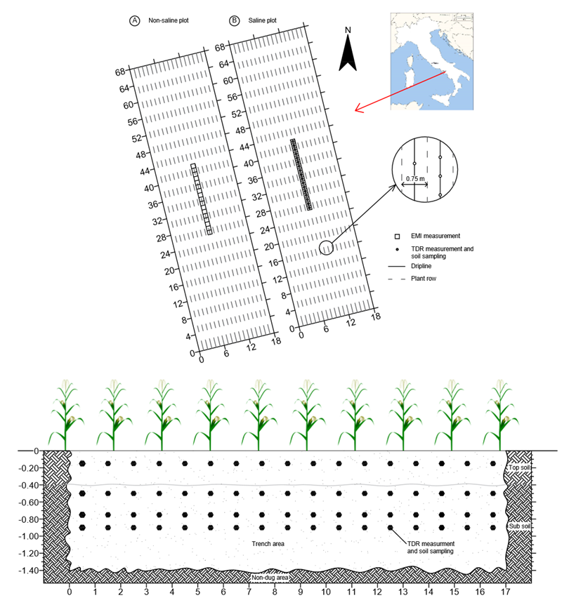
Figure 1 Schematic view of the experimental field (top panel) and front view of the trench showing measurement points (bottom panel). Map of Italy source: https://en.wikipedia.org/wiki/Platania#/media/File:Italy_provincial_location_map_2016.svg (last access: 24 June 2025), licensed under CC BY-SA.

Two plots of silage maize (Zea mays) were arranged in this field, each measuring 18 × 68 m, covering a total area of 1224 m² per plot. The maize was seeded on 16 April 2018 with a row spacing of 0.17 and 0.75 m between adjacent rows and harvested on 2 August 2018 (see Fig. 1, top panel).

Irrigation was performed using a dripline system, consisting of thin-walled polyethylene pipes installed between adjacent plant rows. The system featured drippers spaced 10 cm apart, with a flow rate of 1.5 L h⁻¹. Throughout the growing season, both plots received six irrigation treatments, each providing 490 (±154) m³ ha⁻¹ of water on the same days.

The irrigation water for the non-saline plot was supplied from a farm's well and had a background electrical conductivity of 1.6 dS m⁻¹ with no salt addition In contrast, for the saline plot, calcium chloride (CaCl₂) was added to achieve an electrical conductivity of approximately 8 dS m⁻¹.

During the growing season, the leaf water potential, ψ, was measured on nine dates between 11 June and 29 July 2018 (n=9) on a well expanded, fully light-exposed leaf for each plot using a Scholander type pressure bomb (SAPS II, 3115, Soilmoisture Equipment Corp., Santa Barbara CA, USA). After cutting, the leaf was promptly inserted in the pressure bomb, where pressure was increased at a rate of 0.2 MPa min⁻¹ to determine ψ.

On 2 August, after maize harvesting, apparent soil electrical conductivity (EC_a) measurements were taken on both plots using the CMD Mini-Explorer (GF Instruments, Brno, Czech Republic). This device incorporates three receiver coils positioned at specific distances of 0.32 m (ρ32), 0.71 m (ρ71), and 1.18 m (ρ118) from the transmitter coil, operating at a fixed frequency of 30 kHz. Two coil configurations were utilised with this probe: horizontal coplanar (HCP) and vertical coplanar (VCP) loops. In HCP mode, the instrument's effective depth of investigation is approximately 0.5, 1.0, and 1.8 m for the ρ32, ρ71, and ρ118 coil spacings respectively, whereas VCP mode allows for shallower depth of investigation – approximately half that of the HCP configuration – probing depths of up to 0.25, 0.50, and 0.90 m at the corresponding ρ32, ρ71, and ρ118 coil spacings. This suggests that the instrument offers high vertical resolution for resolving features within the upper 1 m of the subsurface, due to the presence of multiple, closely-spaced measurement points (0.25, 0.5, and 0.9 m effective depths in VCP mode; 0.5 and 1.0 m in HCP mode). The resolution decreases significantly for depths exceeding 1 m because only a single sensor spacing provides data within that deeper range (1.8 m effective depth in HCP mode).

Measurements were acquired along a 17 m-long transect, located centrally in each plot (see Fig. 1, top panel) restricted between two adjacent crop rows to minimize disturbance and avoid spatial aliasing.

On the same day, following the EMI measurements, a 17 m trench was excavated in the saline plot to a depth of 1.4 m, directly along the EMI transect. TDR probes were inserted into 17 vertical profiles within the trench, spaced 1 m apart and positioned at four depths (15, 50, 75, and 90 cm), resulting in a total of 68 measurement points (see Fig. 1, bottom panel). For each point, the Tektronix 1502 C cable tester was used to analyse the acquired wave, measuring the dielectric permittivity (ε) and impedance (Z) over a long time to estimate soil moisture content (θ) and bulk electrical conductivity (σ_b), respectively. This co-location ensured that the surveys referred to the same position as the EMI inversion along the 17 m line.

Notably, TDR measurements were performed in the same positions where time-lapse EMI measurements were previously made, so as to have reference, point-scale values of soil water content and bulk electrical conductivity. Finally, 68 disturbed soil samples were collected in the same locations where TDR measurements were performed to determine soil-solution electrical conductivity (σ_w,SS).

2.2 EMI and TDR analysis

The vertical distribution of bulk electrical conductivity (σ_b(z)) was obtained by inverting the EC_a dataset using EM4SOIL software (Triantafilis et al., 2013) by applying a 1-D laterally constrained method developed by Monteiro Santos (2004). The inversion algorithm employs a set of 1D conductivity models constrained by their neighbours, with forward modelling based on the full solution of Maxwell's equations (Kaufman and Keller, 1983). All models used in the inversion have the same number of layers, and the thickness of these layers is kept constant.

Occam regularization (deGroot-Hedlin and Constable, 1990) and the S2 inversion algorithm (Sasaki, 2001) were utilized in this study. Occam regularization helps to stabilize the inversion process by constraining model variations around a reference model, making the results less sensitive to noisy data. The balance between data fit and neighbour constraints during inversion is controlled by an empirical multiplier (or damping factor). During the inversion process, damping factors values, λ decrease gradually to resolve more detailed parameters (e.g., Farzamian et al., 2019). Inversion results will generally be smoother if the values are larger. The best inversion parameters are usually achieved empirically after testing various parameter sets. In this study, the maximum number of iterations was set to 10, and the damping factor was set to 0.5.

The TDR technique, utilized for both field and laboratory measurements, allows for the estimation of θ and σ_b.

Soil water content is estimated by determining the soil permittivity using the TDR (Tektronix 1502 C), which measures the propagation time of electromagnetic waves generated by the pulse generator and detected by a sampling oscilloscope (Noborio, 2001). Permittivity (ε) is calculated based on the propagation velocity (v) of the electromagnetic waves, as described by:

$$\begin{array}{}\text{(1)}& \mathit{\epsilon }={\left({\displaystyle \frac{c}{v}}\right)}^{\mathrm{2}}={\left({\displaystyle \frac{c\cdot t}{\mathrm{2}L}}\right)}^{\mathrm{2}}\end{array}$$

where c is the velocity of electromagnetic waves in a vacuum (3×10⁸ m s⁻¹), t is the round-trip time for the pulse to traverse the length of the probe (down and back: 2L) [s], L is the TDR probe length [m].

The measurement of σ_b is based on the attenuation of the voltage pulse magnitude (Dalton et al., 1984). The TDR Tektronix 1502 C measures the total resistance, R_T, of the transmission line using:

$$\begin{array}{}\text{(2)}& R_{\mathrm{T}}=R_{\mathrm{s}}+R_{\mathrm{c}}=Z_{\mathrm{c}}{\displaystyle \frac{\left(\mathrm{1}+\mathit{\rho }\right)}{\left(\mathrm{1}-\mathit{\rho }\right)}}\end{array}$$

where: R_c is the series resistance from the cable and connector [Ω], R_s is the soil contribution to the total resistance [Ω], Z_c is the characteristic impedance of the transmission line (50 Ω in this case), ρ is the voltage reflection coefficient at a large travel time, when the signal reflected at the end of the probe reaches a constant value (Comegna et al., 2017).

The σ_b at 25 °C can be calculated as (Rhoades and Van Schilfgaarde, 1976) ${\mathit{\sigma }}_{\mathrm{b}}=K_{\mathrm{c}}/R_{\mathrm{s}}\times f_T$, where K_c is the geometric (cell) constant of the TDR probe and f_T is a temperature correction factor to be used for values measured at temperatures other than 25 °C. Both R_s and K_c can be determined in the laboratory by measuring R_T by TDR in a solution with known salinity.

2.3 Laboratory analysis

2.3.1 Soil-specific θ(ε) relationship

The poorly crystalline clay minerals of Andosols present at the experimental site significantly affect soil dielectric response (Bartoli et al., 2007; Regalado et al., 2003). Consequently, although Topp et al.'s (1980) θ(ε) relationship is generally applicable to most mineral soils, site-specific polynomial relationships were developed for the topsoil and subsoil to ensure accurate soil water content estimation.

To obtain the soil-specific θ(ε) relationship for the investigated soil, preliminarily two PVC cylinders, each with a diameter of 8 cm and a height of 15 cm, were almost filled with air-dried soil to achieve a bulk density of approximately 1.1 g cm⁻³, similar to that of undisturbed soil and a 12 cm long TDR probe was inserted from the top. Then, the soils columns were saturated slowly from the bottom to minimize air entrapment without disturbing packing and allowed complete saturation of the porous media.

To span a wide range of water contents, the columns were then allowed to evaporate at room temperature between measurement cycles. After each evaporation interval, the surface was covered with a thin polyethylene film for one day to promote hydraulic gradient equilibration and the measurements were taken only after this period. At each measurement cycle, a TDR signal was acquired to obtain ε, then the column was immediately weighed, and the film was removed to begin the next evaporation–equilibration cycle. Because TDR integrates along the 10–12 cm rod length, any residual vertical micro-gradients within that domain are effectively averaged (Ferré et al., 1996; Noborio, 2001). At the end of the sequence of 18 measurements, samples were oven-dried at 105 °C for 24 h to determine volumetric water content (θ).

Finally, the resulting θ–ε^0.5 pairs were fitted to a linear relationship $\mathit{\theta }=\mathit{\alpha }+\mathit{\beta }\surd \mathit{\epsilon }$, separately for the Ap and Bw horizons.

2.3.2 Soil-specific θ(σ_b) relationship

To determine the soil specific θ(σ_b) relationship, preliminarily four undisturbed soil samples were collected from the non-saline plot using PVC cylinders (8 cm in diameter and 15 cm in height) to preserve field structure and bulk density. To span different salinity and soil water content, each air-dry sample was subjected to repeated top-wetting increments of 15 mL of CaCl₂ solution at specified electrical conductivities of: 1, 3, 6, and 9 dS m⁻¹. The solution was applied uniformly from the top of the soil core surface and after each increment the sample was covered with 0.05 mm polyethylene film and the core was allowed to equilibrate overnight to promote capillary redistribution of water and solute. This wetting-equilibration procedure was repeated about 20 times for each soil sample to cover a wide range of soil water content values, from air-dry (θ≈0.06 cm³ cm⁻³) to near saturation (θ≈0.46 cm³ cm⁻³) with increases in water content of approximately 0.02 cm³ cm⁻³ for each application. For each sample, the procedure was stopped when the application volume led to visible drainage of the soil solution from the bottom of the cylinder.

For each soil sample, at the beginning of the experiment, a three-wire TDR probes (10 cm long with a rod diameter of 0.3 cm and rod spacing of 1.2 cm) was vertically inserted into the soil columns. Measurements of volumetric water content (θ) were taken using the topsoil-specific θ(ε) relationships, and bulk electrical conductivity (σ_b) was also measured, based on the TDR impedance, Z, obtained at large signal travel times (e.g., Robinson et al., 2003).

The θ–σ_b relationship calibration was obtained by ordinary least squares on the low-salinity subset (σ_w≈1 dS m⁻¹) and restricted to the medium-to-high θ range, representative of irrigation-season conditions, to avoid the known non-linearity and reduced sensitivity at low θ. Given the overall soil homogeneity, an unique linear fits $\mathit{\theta }=a+b{\mathit{\sigma }}_{\mathrm{b}}$ were derived for whole profile.

2.3.3 Calibration of the Rhoades θ–σ_b–σ_w model

Rhoades et al. (1976) proposed a linear model between σ_b and σ_w for a given θ value:

$$\begin{array}{}\text{(3)}& {\mathit{\sigma }}_{\mathrm{b}}=\mathit{\theta }T{\mathit{\sigma }}_{\mathrm{w}}+{\mathit{\sigma }}_{\mathrm{s}}\end{array}$$

were T is the transmission coefficient, also known as tortuosity, which considers the tortuous nature of the current line and any decrease in the mobility of the solid-liquid and liquid-gas interfaces, whereas σ_s represents the electrical conductivity of the solid phase of the soil that is associated to the exchangeable ions in the solid-liquid interface.

Tortuosity linearly depends on θ and is characterised as follows:

$$\begin{array}{}\text{(4)}& T=a\mathit{\theta }+b\end{array}$$

where a and b are parameters specific for each soil type estimated as a fitting parameter in Eq. (3). σ_s is calculated using a graphical approach (Rhoades et al., 1976).

In order to calibrate the Rhoades model for deriving the soil-specific a, b and σ_s parameters, the procedure was performed separately for Ap and Bw soils, using the undisturbed cores and the stepwise wetting protocol described in Sect. 2.3.2 (CaCl₂ solutions at σ_w=1, 3, 6, 9 dS m⁻¹; room temperature). This “increment-and-equilibrate” approach mirrors standard TDR laboratory practice for jointly acquiring ε and σ_b on the same volume and at stable moisture/salinity states as reported in Malicki and Walczak (1999) Finally, the obtained θ–σ_b–σ_w data were fitted to the Rhoades model to finalize the calibration procedure. To do this, parameters (a, b and σ_s) were estimated by nonlinear least squares (Levenberg–Marquardt), minimizing the sum of squared residuals between measured and predicted σ_b values. Non-negativity constraints were imposed σ_s≥0. The best-fit coefficients of the calibration procedure (RMSE an R²) are reported Table 1.

2.3.4 Soil solution electrical conductivity determination

The soil solution electrical conductivity (σ_w,SS) was determined on 1 , 2 volume extract method (Rhoades et al., 1999). The 68 disturbed soil samples collected from the trench were preliminary air dried at room temperature, crumbled and sieved through a 2 mm mesh to remove coarse fragments and roots before extraction. Subsequently, for each sample, a 1 : 2 soil-to-water suspensions were prepared using 50 g of soil and 100 mL of distilled water. Once the soil and water were combined, the suspension was stirred thoroughly to ensure the full dissolution of the soluble salt into the water. After mixing, the suspension was centrifuged to separate the solid particles from the liquid phase, allowing extract the soil solution. Finally, the electrical conductivity of the extracted soil solutions was measured using a calibrated EC meter (Alves et al., 2022). Subsequently, chloride concentration in the extracts was determined via titration (Mohr's Method). A linear regression model was then established between the measured electrical conductivity (σ_w,SS) and the corresponding chloride concentration, resulting in an empirical relationship of the form:

$$\begin{array}{}\text{(5)}& {\mathit{\sigma }}_{\mathrm{w},\mathrm{SS}}=\mathrm{0.0028}\left[{\mathrm{Cl}}^{-}\right]+\mathrm{0.068}\end{array}$$

where σ_w,SS is the electrical conductivity of extract (dS m⁻¹), [Cl⁻] is the chloride concentration (mg L⁻¹).

To estimate the electrical conductivity representative of field conditions, the chloride concentration was scaled to the measured soil water content (SWC) of each sample. The scaled chloride concentration was calculated as the ratio between the total chloride mass and the water mass in the soil sample. Finally, the scaled [Cl⁻] was used in Eq. (5) to estimate the electrical conductivity, representative of the soil solution under its field water content conditions (σ_w,SS).

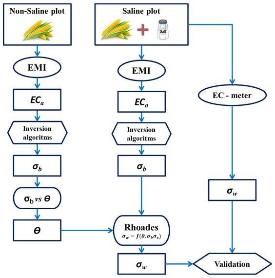
2.4 A synthesis of the applied procedure

The flowchart of the proposed procedure is displayed in Fig. 2 and summarized in the following six steps:

• 1.

  Irrigation and EMI Measurements: Two adjacent maize plots, were irrigated with saline and plain water, respectively. EMI measurements were performed along a 17-transect in middle of each plot in order to obtain the distribution of the EC_a within the two plots.

• 2.

  Inversion of EC_a to obtain σ_b: The σ_b distribution in both plots was calculated using the inversion procedure, detailed in Sect. 2.2.

• 3.

  Soil-specific laboratory calibrations

  • i.

    θ(ε) relationship: A relationship θ(ε) was determined in laboratory on non-saline soil comparing soil-specific θ–√ε relations with the Topp et al. (1980) polynomial and the Ferré linearization.

  • ii.

    θ(σ_b) relationship: A linear calibration of θ–σ_b relationship was determined on soil from the non-saline plot.

  • iii.

    Rhoades θ–σ_b–σ_w model: A θ–σ_b–σ_w Rhoades et al. (1976) model parameters a, b and σ_s were estimated from laboratory dataset separately for the two horizons.

• 4.

  Determination of θ distribution in non-saline plot: The inverted σ_b dataset obtained from the non-saline plot (Step 2) was converted in θ by the horizon-specific θ–σ_b relation (Step 3-ii).

• 5.

  Estimation of σ_w in the saline plot: The inverted σ_b dataset from the saline allowed to estimate σ_w using the Rhoades et al. (1976) model and the average soil water content determined in the step 4. This estimation was based on the assumption that the mean and the variance of the soil water content distribution were similar in both plots.

• 6.

  Validation of σ_w and θ

  • i.

    The σ_w values estimated using the described procedure were validated by comparison to an independent σ_w dataset obtained in the laboratory through soil solution electrical conductivity (EC) measurements on disturbed soil samples (σ_w,SS).

  • ii.

    The θ values estimated by EMI were validated by comparing the soil water content measured with TDR in the saline plot.

  The reliability of the estimates was analysed based on root mean square values (Root Mean Square Error, RMSE) and the mean deviation (Bias), according to the following formulas:

  $$\begin{array}{}\text{(6)}& {\displaystyle }\mathrm{RMSE}=\sqrt[\mathrm{2}]{{\displaystyle \frac{\sum _{i=\mathrm{1}}^n{\left(X_{\mathrm{m},i}-X_{\mathrm{es},i}\right)}^{\mathrm{2}}}{N}}}\text{(7)}& {\displaystyle }\mathrm{Bias}={\displaystyle \frac{\sum _{i=\mathrm{1}}^n(X_{\mathrm{es},i}-X_{\mathrm{m},i})}{N}}\end{array}$$

  where X_m are the measured values, X_es are the estimated values at the time i and N is the number of measured values.

Figure 2 Flowchart of the proposed procedure.

3 Results and Discussion

3.1 Field EC_a acquisition in the non-saline plot [Step 2]

Figure 3 reports the spatial distribution of the measured apparent soil electrical conductivity (EC_a) under VCP configuration (a) and HCP configuration (b) for the three receiver coils ρ32, ρ71, and ρ118. The EC_a values are generally low, ranging from 0.02 to 0.08 dS m⁻¹. The EC_a data exhibit a similar pattern in both VCP and HCP modes, with slightly higher EC_a values at ρ118, intermediate values at ρ71, and lower values at ρ32. This trend suggests a more conductive zone at deeper layers. In terms of horizontal variability, the EC_a in vertical mode shows relatively small variation, with coefficients of variation of 15 %, 14 %, and 13 % for ρ118, ρ71, and ρ32, respectively. Even lower are the coefficients of variation in horizontal mode. Looking at the transect in Fig. 6a, an anomalous behaviour is revealed between 4.8 and 6.4 m. This anomaly is attributed to an old buried channel crossing the plot, which was uncovered during the excavation of the trench along the transect. Although the soil within the channel, formed over more than 80 years, had undergone pedogenesis and appeared similar to the surrounding soil, the channel's contours remain distinct and recognizable.

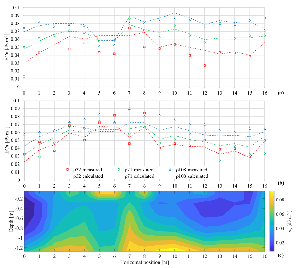
Figure 3 Apparent soil electrical conductivity (EC_a) along the transect for the non-saline plot: (a) HCP mode; (b) VCP mode. Points indicate measured EC_a, while dashed lines show the calculated EC_a (forward response of the inversion). (c) Inversion results showing the bulk electrical conductivity (σ_b) distribution with depth.

Figure 3c presents the modelling results with estimation of σ_b distribution with depth, down to 1.2 m, along the profile. The maximum depth for the presented model was selected based on the expected vertical resolution of the sensor (see Sect. 2.2) and investigation depth of interest where supporting data were available. The model response was shown in Fig. 3a, b by dashed lines. The misfit error is 0.01 dS m⁻¹, indicating a fairly good fit between the observed data and model responses. In terms of vertical variability, the σ_b values follow the trend of the observed data, showing a general increase with depth. This pattern suggests the presence of at least three distinct electrical layers, each with unique electrical and electromagnetic properties:

In the surface layer (0–30 cm), electrical conductivity exhibits medium-to-high values (0.03–0.08 dS m⁻¹), likely due to a combination of factors. These include low soil water content during the EMI measurement and a slight increase in salt concentration in the pore water caused by evaporation from the soil surface, which is wetted by surface drip irrigation. Furthermore, as reported by Bonfante et al. (2019), who studied the same soil, the upper layer has a higher clay content (10.5 %) compared to the underlying layers. Given the well-established strong correlation between EC_a and clay content (Sudduth et al., 2005), it is reasonable to hypothesize that the clay content could influence the observed EC_a patterns in this surface layer.

The central layer (30–80 cm) is characterized by a minimum in σ_b values forming a gradient that decreases from the top to the bottom of this layer. This zone is wetted by downward percolation (wetting bulb) from the drip surface irrigation, coinciding with peak root activity and also a decrease in clay content from 5.9 % to 3.9 % (Bonfante et al., 2019). Moreover, this layer is likely affected by downward leaching of salts and fertilizers toward deeper layers with drip irrigation water (Corwin et al., 2022).

The third and deepest layer (below 90 cm) is characterized by a progressive increase in bulk electrical conductivity. This can be explained by the highest clay content in soil profile (11.6 %), combined with an increase in soil compaction with depth that reduces water storage capacity, related to the reduction of porosity in this zone.

Regarding lateral variability, the overall variability remains low across all depths, except for the zone corresponding to the old channel, which is clearly distinguishable. The presence of this channel likely contributes to localized differences in soil properties, (such as the bulk density), creating distinct pattern in the electrical conductivity profile.

3.2 Laboratory experiments

3.2.1 Soil-specific θ(ε) relationship [Step 3.i]

Table 1 presents the coefficients α and β for the linear soil-specific relationship $\mathit{\theta }=\mathit{\alpha }+\mathit{\beta }\surd \mathit{\epsilon }$, along with the coefficient of determination (R²) for both topsoil (Ap horizon) and subsoil (Bw horizon), obtained from laboratory experiments. The equations for the Ap horizon and Bw horizon show similar intercepts but slightly different slopes, leading to a divergence between the two curves at higher soil water contents.

Table 1 Coefficients and R² values for the θ–√ε, θ–σ_b, and θ–σ_b–σ_w soil-specific calibration relationships

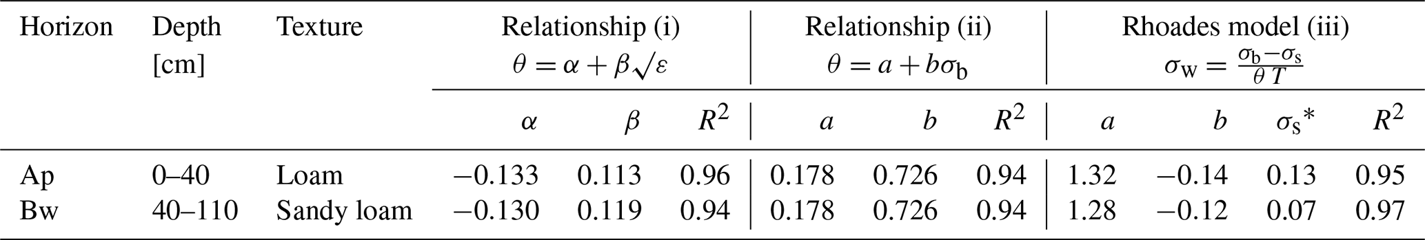
^* [dS m⁻¹].

Figure 4 compares the two observed relationships with the linear form of Topp's equation. The findings indicate that Topp's equation consistently overestimates the water content, with an average overestimation of approximately 0.07 ± 0.01 cm³ cm⁻³ in the Ap horizon and about 0.05 ± 0.02 cm³ cm⁻³ in the Bw horizon. These discrepancies suggest that the application of Topp's equation may require local calibration to account for horizon-specific characteristics.

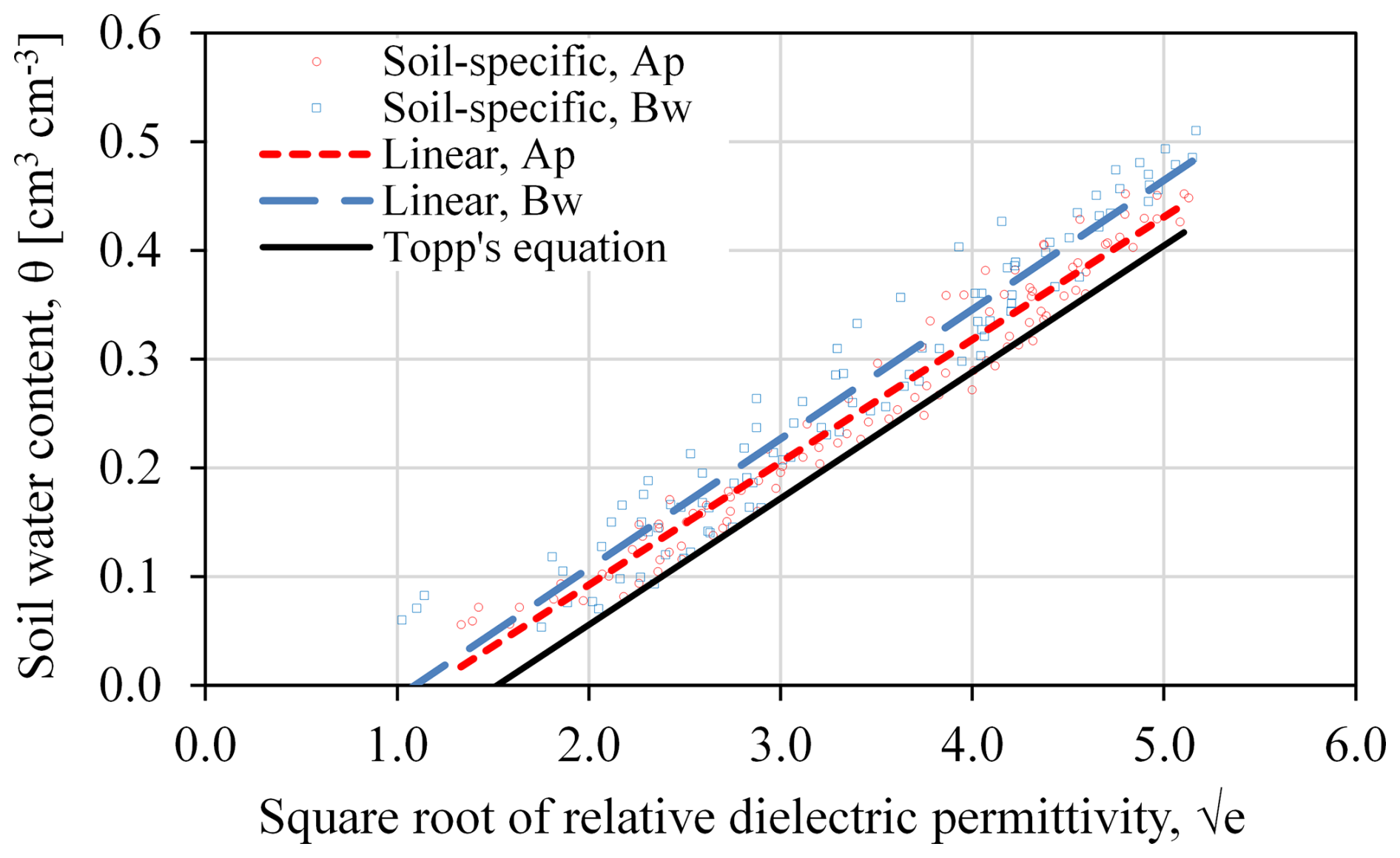
Figure 4 Soil specific linear relationship between the square root of relative dielectric permittivity and volumetric soil water content for the Ap and Bw horizons.

3.2.2 Soil-specific θ(σ_b) relationship [Step 3.ii]

Figure 5 shows the soil-specific linear calibration between soil water content and bulk soil electrical conductivity $\mathit{\theta }=a+b{\mathit{\sigma }}_{\mathrm{b}}$, with separate fit for the Ap and Bw horizons. Table 1 shows the corresponding coefficients of the relationship, along with the coefficients of determination (R²).

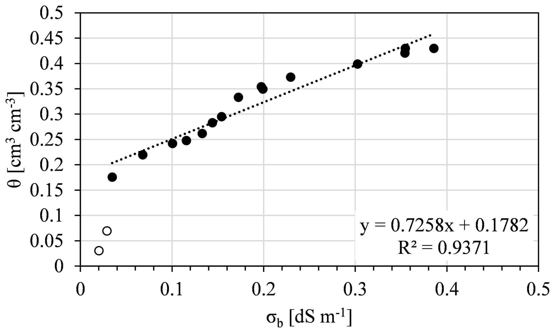
Figure 5 Soil specific linear relationship between the σ_b and volumetric soil water content for whole soil profile. The filled circle indicates the θ–σ_b pairs from measured values, the dotted line represents the linear regression while the circles whit the white background are the pairs excluded from the calibration of the linear relationship.

3.2.3 Calibration of the Rhoades θ–σ_b–σ_w model [Step 3.iii]

Figure 6 presents the results of the laboratory experiment conducted using TDR to calibrate the parameters of the Rhoades et al. (1976) model (also reported in Table 1). For each soil water content, ranging from 0.15 to 0.40 cm³ cm⁻³, σ_b increases linearly with σ_w within a range of 1 to 9 dS m⁻¹. The σ_s values at different soil water content levels converge towards 0.13 dS m⁻¹ for topsoil and 0.07 dS m⁻¹ for subsoil.

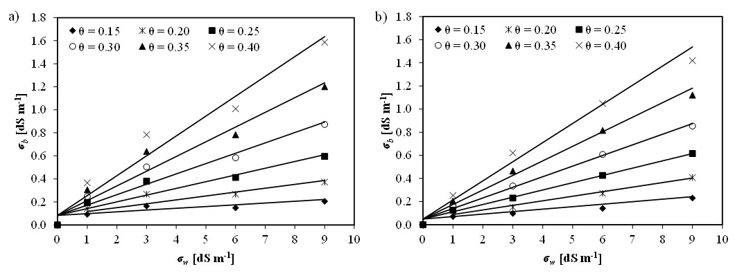
Figure 6 Bulk electrical conductivity (σ_b) measured by TDR vs. pore water electrical conductivity (σ_w) measured by an EC meter for six levels of soil water content (cm³ cm⁻³). The continuous lines represent the fitted Rhoades model (Eqs. 1 and 2) for (a) topsoil and (b) subsoil.

It's important to note that this relationship does not apply under dry soil conditions. In fact, the graphs show that as the water content decreases, the slope of the fitting line progressively flattens, becoming nearly horizontal at θ=0.15 cm³ cm⁻³. This suggests that σ_b becomes almost insensitive to changes in σ_w as the soil dries (Nadler, 1982; Rhoades et al., 1989). According to Nadler (2005), the relationship at low θ values becomes impractical due to the complex interdependencies between various solid- and liquid-phase parameters that dominate as water content decreases.

This finding is crucial for this study's focus on using EMI for salinity and water content assessment, as it indicates that EMI measurements should be conducted in wet or moderately wet soils rather than dry soils. Moreover, it highlights that a reasonable soil moisture threshold for reliable measurements in the studied soil is greater than 0.15 cm³ cm⁻³.

3.3 Determination of θ distribution in non-saline plot [Step 4]

Figure 7 presents the θ values at four distinct depths (15, 50, 75, and 90 cm), derived from the soil-specific θ(σ_b) relationships detailed in Table 1 and correspond to the depths extracted from the image shown in Fig. 6c.

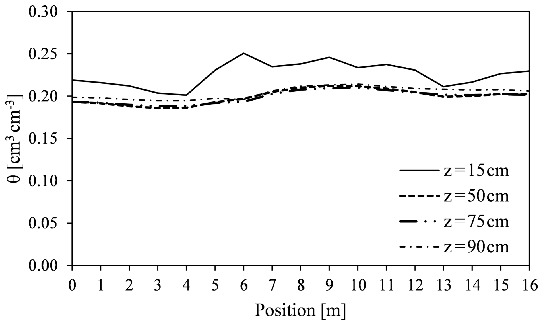
Figure 7 Spatial distribution of soil water content (θ) in the non-saline plot at four depths (15, 50, 75, and 90 cm), estimated from bulk electrical conductivity (σ_b) distribution.

At depths of 50, 75, and 90 cm, the θ data series nearly overlap, with average soil water content values 0.20 cm³ cm⁻³. The variability at these depths is minimal, with an average coefficient of variation of 3.9 %. In contrast, the upper layer (15 cm) shows a higher average soil water content of 0.23 cm³ cm⁻³ and greater variability, with a coefficient of variation of 6.3 %. This suggests that deeper soil layers maintain more stable moisture conditions, while the upper horizon is more influenced by processes at boundary such as evaporation and infiltration.

Across all depths, higher values of soil water content are observed in the central part of the transect (7–12 m). This pattern corresponds to the higher σ_b values shown in the data presented in Fig. 6c, indicating an increase in soil water content in this section of the plot across the different depths.

3.4 Estimation of σ_w in the saline plot [Step 5]

Figure 8a shows the EC_a measurements in both VCP and HCP modes for the three receiver coils ρ32, ρ71, and ρ118. The EC_a values are higher than those observed in the non-saline plot, ranging from 0.2 to 0.45 dS m⁻¹. Both VCP and HCP data display a similar pattern, with EC_a values decreasing from the upper layer to the deeper layer, suggesting a more conductive topsoil, which is expected due to saline water irrigation. The differences are more pronounced in the VCP mode compared to the HCP mode. In terms of lateral variability, the EC_a in vertical mode exhibits relatively minor variation, with coefficients of variation of 15 %, 14 %, and 13 % for ρ118, ρ71, and ρ32, respectively. Additionally, higher EC_a values are observed in the central part of the plot, gradually decreasing towards the edges. Despite the presence of the old buried channel crossing the plot, no noticeable differences in EC_a are evident along this transect. This can be attributed to the dominant impact of soil salinity which masks the channel impact. The contribution of the channel is relatively minor (around 0.02 dS m⁻¹), as previously observed in Fig. 6a.

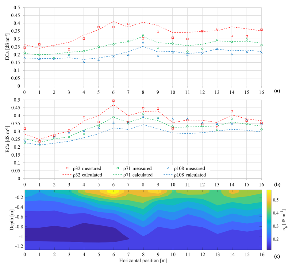
Figure 8 Apparent soil electrical conductivity (EC_a) along the transect for the saline plot: (a) HCP mode; (b) VCP mode. Points indicate measured EC_a, while dashed lines show the calculated EC_a (forward response of the inversion). (c) Inversion results showing the bulk electrical conductivity (σ_b) distribution with depth.

Figure 8c shows the σ_b distribution obtained from the inversion procedure of the EMI measurements conducted on 2 August in the saline plot. The model response was shown in Fig. 8a, b by dashed lines. The misfit error is 0.03 dS m⁻¹, indicating a fairly good fit between the observed data and model responses. The misfit is slightly higher than the one observed in non-saline soil, due to greater EC_a values and variability range. As expected, the values of σ_b obtained from the inversion modelling were consistently higher in the saline plot compared to the non-saline plot. These values decreased from the surface to a depth of two metres, ranging from 0.55 to 0.10 dS m⁻¹. This pattern of declining σ_b with depth has also been reported by other authors (e.g., Saeed et al., 2017). During the irrigation season, salt accumulation tends to be concentrated in the topsoil layer (Coppola et al., 2015, 2016), largely due to evaporation at the soil surface, which causes salts to rise and concentrate in the upper layers (Corwin and Lesch, 2005; Kara and Willardson, 2006).

The Rhoades model was applied to estimate the electrical conductivity of the soil solution based on the σ_b measurements obtained from the EMI for both horizons. The laboratory calibrations provided the parameters a, b, and σ_s (as shown in Table 1), while θ was assumed as the average value measured in the non-saline plot (an average value for each of the four depths, as seen in Fig. 7). In addition, to account for the variability of water content in the non-saline plot – and consequently, the error associated with its estimation, which influences the σ_w estimation procedure – the analysis was also conducted by using the mean water content value plus or minus its standard deviation. In this way, the validity of using the average value of the non-saline plot was numerically tested and further supported by additional considerations discussed in Sect. 3.5.

3.5 Validation of σ_w and θ

3.5.1 σ_w: estimated by EMI (σ_w,EMI) vs. soil solution (1 : 2) extract (σ_w,SS) [Step 6.i]

Validation of the soil electrical conductivity estimated by EMI, σ_w,EMI, was carried out by comparing it with soil solution electrical conductivities measurements, σ_w,SS. Figure 9 illustrates the results for four depths: 15, 50, 75, and 90 cm. In the figures, the data series for σ_w,EMI are represented by continuous lines, while σ_w,SS values are shown as squares. To account for small-scale heterogeneity in σ_w,SS – arising from the differing observation scales of the two data series – a simple moving average filter was applied to smooth the σ_w,SS data. As a result, the influence of individual measurements (short-term fluctuations) was minimized, while preserving the overall trend along the transect (long-term fluctuations) (Dragonetti et al., 2018; Western and Blöschl, 1999).

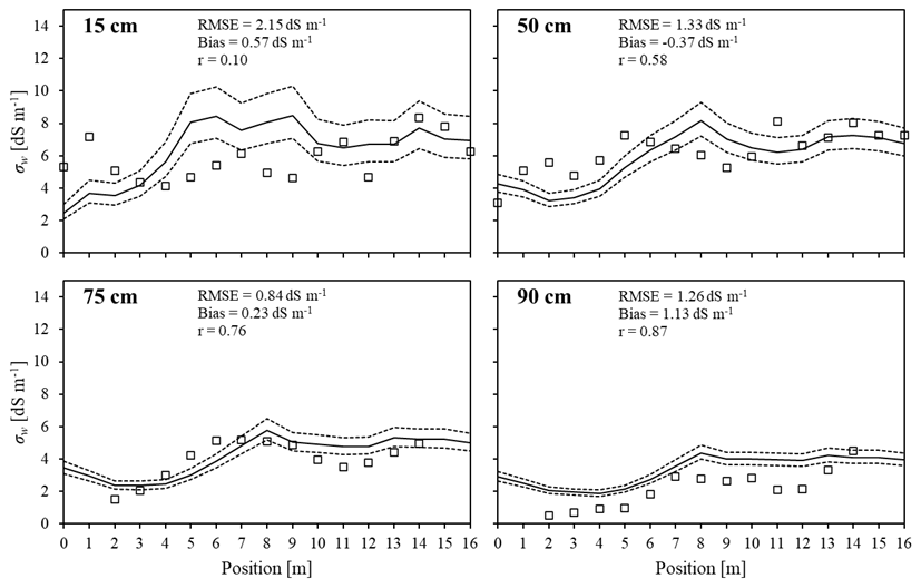
Figure 9 Spatial distribution of σ_w within the trench at four depths (15, 50, 75 and 90 cm). The continuous lines represent σ_w,EMI, while the squares indicate the measured σ_w,SS after applying a filtering process. The dotted lines denote the variability range of σ_w,EMI, computed based of one standard deviation of θ as measured in the non-saline plot.

The largest discrepancies between measured and estimated σ_w values occur at a depth of 15 cm, with significant scatter around the mean (RMSE = 2.15 dS m⁻¹) and a relatively high overestimation (bias = 0.57 dS m⁻¹). At the other three depths, the data show better agreement, with RMSE values below 1.33 dS m⁻¹ and bias ranging from −0.37 to 1.13 dS m⁻¹.

As depth increases, the correlation coefficient between the two series rises from 0.10 in the upper layer to 0.87 in the deeper layer. The graphs in Fig. 9 also show the σ_w,EMI estimates obtained by assuming, at each depth considered, the average plus/minus the standard deviation of the water contents measured under the non-saline transect (dotted lines). Note that the uncertainty in the σ_w,EMI estimations coming from the assumption of similarity between the two plots in terms of water contents is quite high only for the data at 15 cm. This uncertainty decreases markedly with depth, likely due to reduced variability in soil water content. This issue is discussed in detail later in a dedicated section.

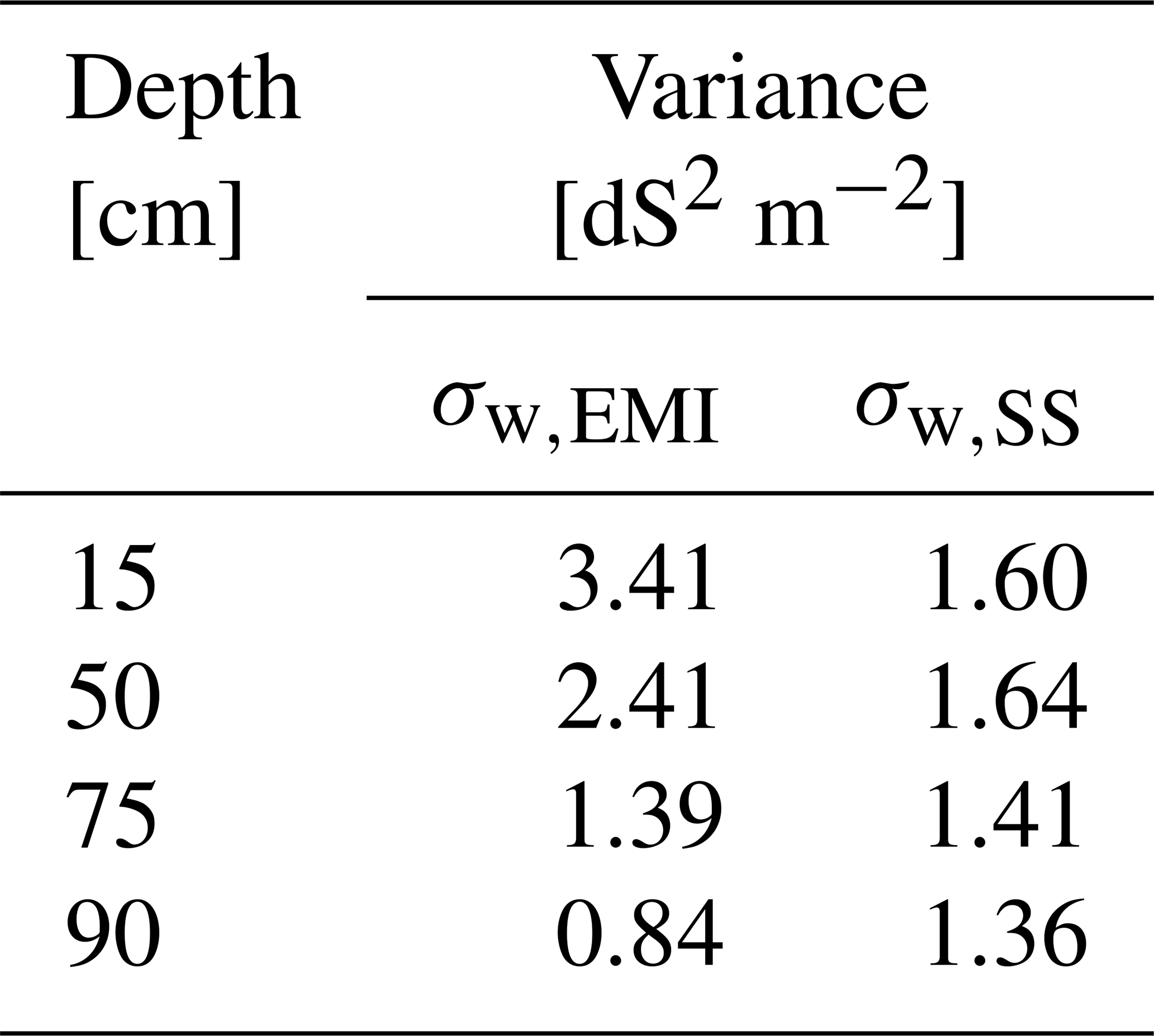
As suggested by Robinet et al. (2018) who analysed the reasons behind discrepancies in σ_b detected by sensors operating at different observation volumes – similar to our case – the weak correlation between EMI and soil sampling measurements for a shallow sensing coil configuration and the forward-calculated EC_a can be attributed to several factors. Firstly, significant variations in σ_b near the soil surface may not be effectively captured by local soil sampling. Secondly, the uneven and irregular nature of the soil surface can significantly impact EMI measurements. Variations in elevation and rough terrain make it difficult for the operator to keep the instrument at a constant height above the ground. Since EMI measurements are highly sensitive to the distance between the sensor and the soil, any fluctuations in height can introduce inconsistencies in the data, potentially affecting the accuracy and reliability of the results. Thirdly, σ_b measurements are influenced by the maize root system, which is denser in the shallower soil layer, further impacting the readings. These factors contribute to the relatively high variance observed at 15 cm in EMI measurements (σ_w,EMI), which decreases with depth (see Table 2). By contrast, the same table shows that the variance σ_w,SS remains roughly constant, with a slight decrease toward depth.

Table 2 Values of variance for the σ_w measurement by EMI, σ_w,EMI, soil solution, σ_w,SS and filtered soil solution data.

3.5.2 EMI vs. TDR (saline plot) [Step 6.ii]

The procedure was further validated by comparing the soil water content estimated by EMI with an independent series of water content measurements taken by TDR in the saline plot immediately after the EMI readings. While this comparison was not strictly required for the procedure, it serves to corroborate the assumptions and findings discussed. In fact, the concept of validation has a twofold meaning. On one hand, it allows us to assess whether the estimated values, obtained through the six-step procedure outlined in Fig. 1, align with the measured ones. On the other hand, it verifies whether the value estimated from the non-saline plot effectively corresponds to the one measured in the same plot. Additionally, validation provides insights into the variability of the estimate compared to the actual measurements.

Figure 10 presents the data series for soil water content estimated by EMI (θ_EMI), derived from EMI measurements following the outlined procedure, shown as continuous lines. Alongside these, the measured water content values from TDR (θ_TDR) are represented by filled squares. Each panel in Fig. 10 also includes statistical parameters − root mean square error (RMSE), bias, and correlation coefficient (r) − which assess the agreement between the θ_EMI and θ_TDR series.

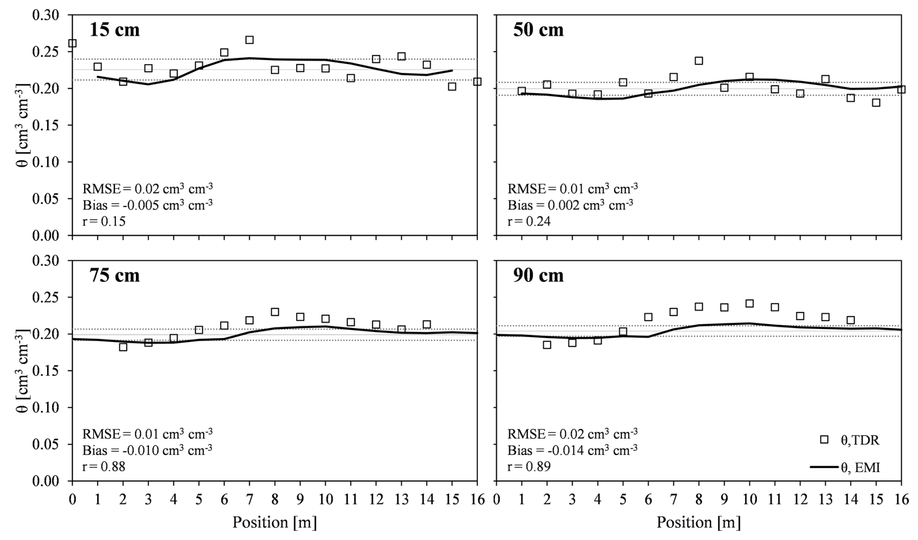
Figure 10 Spatial distribution of soil water content within the trench for four depths (15, 50, 75 and 90 cm) as measured by TDR (θ_TDR) and estimated by EMI, (θ_EMI) in the non-saline transect. The θ_TDR data are represented by empty square. θ_EMI data for each position are represented by a continuous thick solid line. Horizon-wise mean of θ_EMI value is represented by a thin solid line while dashed lines represents the horizon-wise θ_EMI mean ± SD.

The water content at each depth remains approximately constant throughout the transect, indicating notable homogeneity in the horizontal plane. This observation supports the fundamental hypothesis of the study. Across the four depths, the average values of θ_EMI ranged between 0.20 and 0.23 cm³ cm⁻³, with a mean error (RMSE) of 0.02 cm³ cm⁻³ and a slight underestimation whit a BIAS value of −0.008 cm³ cm⁻³.

A weak correlation was observed in the topsoil, where the correlation coefficient between θ_EMI and θ_TDR was low, with values of r=0.15 and 0.24 at depths of 15 and 50 cm, respectively. In contrast, a strong correlation was observed in the subsoil at depths of 75 and 90 cm, with r values of 0.88 and 0.89, respectively. This trend of increasing correlation from topsoil to subsoil is consistent with previous studies, such as Calamita et al. (2015), which reported similar patterns.

The dotted lines in the four plots of Fig. 10 represent the range of variability of σ_w,EMI, calculated adding and subtracting the standard deviation (SD) of θ from the values measured in the non-saline plot for each layer. These two lines help to quantify the impact of using the average θ obtained at different depths in the non-saline transect when analysing data from the saline transect.

Regarding correlation and RMSE, the impact of soil water content variability on the σ_w estimate decreases with increasing measurement depth. At 15 cm the effect is relatively pronounced, whereas at greater depths it becomes negligible. This finding underscores the robustness of the obtained values, with minimal uncertainty at deeper layers. However, at 15 cm the estimates are less reliable. In fact, various studies have highlighted the impact of θ variability on soil salinity estimation, particularly within the root zone, where significant fluctuations in θ occur due to irrigation practices and evaporation (e.g., Gómez Flores et al., 2022; Paz et al., 2020).

3.6 Limits and conditions of use of the procedure

The procedure assumes that, on the surveys date, the average horizon-wise soil water content in the saline plot is similar to that in the non-saline plot. In the context of our case study, this assumption is supported by the following considerations:

• 1.

  Pedo-hydrological similarity:

  A study by Bonfante et al. (2019) conducted at the same site demonstrated the pedo-hydrological similarity between the two plots. Their Fig. 2 illustrates that the soils and horizons in both plots exhibit very similar hydrological and physical properties.

• 2.

  Identical field management:

  Throughout the growing season, both plots were managed identically:

  • –

    They received the same irrigation volumes and followed the same irrigation schedule.

  • –

    Maize was sown on the same day in both plots.

  • –

    The first saline irrigation was applied on 6 June – approximately 50 d after sowing (16 April) – to prevent early stress and minimize its impact on crop development.

  • –

    Physiological measurements, including phenological phase and root depth, were comparable across both plots.

• 3.

  Water Uptake and Crop Response:

  • –

    Leaf water potential measurements showed no significant differences throughout the irrigation. A t-test confirmed the absence of significant differences between the plots (p>0.05), indicating similar water uptake conditions.

In summary, given the nearly identical soil and sequence of soil horizons, their corresponding hydraulic properties, and the identical irrigation regime, it is reasonable to assume that the mean water content in each horizon on the survey date is similar in both plots. This assumption is further supported by the mostly overlapping water uptake and physiological status of maize during the irrigation season. Consistently with this assumption, the horizon-wise mean θ required by the Rhoades model was obtained in the non-saline plot from EMI via the site-specific θ–σ_b calibration. A concurrent experiment at the same experimental farm (Bonfante et al., 2019) collected a single vertical TDR profile in the non-saline plot on the survey date. The measured θ values on these surveys were consistent with the EMI-derived horizon-wise means; however, this profile is not presented here because its spatial representativeness is limited and its inclusion would not affect the analyses or conclusions.

In a context of relative soil homogeneity and similar agricultural management, the procedure yielded satisfactory results. Therefore, the procedure effectiveness diminishes when applied on a larger scale or to heterogeneous soil conditions. In addition, accuracy is expected to be lower in the upper 10–20 cm where EMI sensitivity decreases and near-surface θ dynamics are stronger.

However, if the experimental conditions revealed at the site here described are not available, the applicability of the method may be challenged. In such cases, adjustments would help ensure the reliability and robustness of the procedure in different environmental and agronomic contexts. Specifically, when a twin of non-saline plot is not available, the horizon-wise mean θ on the survey date can be obtained directly in the field using a small set of moisture probes placed in homogeneous zones identified by a preliminary EC_a map. Moreover, EMI shortly after irrigation/rainfall further reduces θ contrasts.

In principle, the procedure is specifically designed for soils experiencing secondary salinization due to irrigation, which facilitates the identification of similar non-saline soils on the same farm. Applying this procedure to soils with primary salinization is more challenging, due to the absence of such reference conditions. Nevertheless, this limitation is partially addressable. The average soil water content for each layer could be independently measured using alternative methods and applied directly to the saline plot, thereby eliminating the need for a reference non-saline plot. For instance, installing a network of soil moisture probes adequately calibrated and strategically placed across the field could provide the necessary data to apply the proposed methodology. In this case, the adequate placement of soil moisture sensors plays a crucial role in ensuring the representativeness and accuracy of the measurements. Variability field maps derived from EC_a measurements could be used preliminary to identify zones with homogeneous soil properties and the sensors could be strategically positioned within these zones to capture a comprehensive profile of soil water content required to apply the proposed procedure extensively throughout the field. In such applications, uncertainty can be transparently conveyed by propagating the horizon-wise θ mean ± SD used in the inversion. This solution could be broadening the potential applicability of the procedure to other contexts, eliminating the need for a non-saline plot and considering the soils spatial variability.

4 Conclusions

This study introduces a novel procedure for quickly distinguishing the contributions of water content and salinity in electromagnetic induction (EMI) measurements of apparent electrical conductivity (EC_a) providing a valuable tool for soil and water management. EC_a measurements were conducted along two adjacent parallel transects: one irrigated with non-saline water and the other with saline water. Electrical conductivity levels of 1 dS m⁻¹ (considered the non-saline level) and 8 dS m⁻¹ were utilized for comparison.

The proposed procedure is based on the hypothesis that the average soil water content in the saline transect is “similar” to that in the adjacent non-saline transect. Given the similar soil physical properties, hydrology, irrigation distribution, and fertilization practices expected in both transects, we anticipate comparable agronomic conditions. This can lead to similar root distributions and nutrient uptake patterns, ultimately resulting in analogous water content distributions. Our findings support the validity of this hypothesis, as evidenced by the strong correlation between σ_w estimated via EMI and σ_w measured directly from soil solutions extracted from samples.

When the hypothesis holds, the proposed procedure is relatively straightforward to implement, addressing a key challenge in EMI application, distinguishing the effects of soil water content and salinity. To the best of our knowledge, this represents the first field-scale attempt to differentiate these effects in EMI measurements.

Despite the promising results, certain limitations must be acknowledged. Firstly, the underlying assumption of similar average soil water content limits the applicability of the proposed procedure, and, therefore, the procedure's effectiveness diminishes when applied on a larger scale or to heterogeneous soil conditions. Secondly, the procedure is specifically designed for soils experiencing secondary salinization due to irrigation, which facilitates the identification of similar non-saline soils on the same farm. Applying this procedure to soils affected by primary salinization is more challenging, because a comparable non-saline reference plot is typically unavailable.

Finally, the reliability of the EMI method tends to diminish at the soil surface, which can lead to less accurate results. however, with the fast development of EMI sensors equipped with a greater number of receivers and/or frequencies, the accuracy of EMI at soil surface may improve to some extent.

Future research should aim to validate the hypothesis of similar water content distribution in shallower soil layers, which often exhibit more erratic dynamics and less consistent results. To enhance this validation, the proposed procedure could be integrated with simulations of soil water flow using hydrological models, alongside appropriate top boundary conditions applied in the field experiment.