the Creative Commons Attribution 4.0 License.
the Creative Commons Attribution 4.0 License.
 | 06 Aug 2020
Disaggregating a regional-extent digital soil map using Bayesian area-to-point regression kriging for farm-scale soil carbon assessment
Sanjeewani Nimalka Somarathna Pallegedara Dewage
Budiman Minasny
Brendan Malone
Most soil management activities are implemented at farm scale, yet digital soil maps are commonly available at regional or national scale. Disaggregating these regional and/or national maps is applicable for farm-scale tasks, particularly in data-poor or limited situations. Although disaggregation is a frequently discussed topic in recent digital soil mapping literature, the uncertainty of the disaggregation process is not often discussed. Underestimation of inferential or predictive uncertainty in statistical modelling leads to inaccurate statistical summaries and overconfident decisions. The use of Bayesian inference allows for quantifying the uncertainty associated with the disaggregation process. In this study, a framework of Bayesian area-to-point regression kriging (ATPRK) is proposed for downscaling soil attributes, in particular, maps of soil organic carbon. An estimation of point support variograms from block-supported data was carried out using the Monte Carlo integration via the Metropolis–Hastings algorithm. A regional soil carbon map with a resolution of 100 m (block support) was disaggregated to 10 m (point support) information for a farm in northern New South Wales (NSW), Australia. The derived point support variogram has a higher partial sill and nugget, while the range and parameters do not deviate much from the block support data. The disaggregated fine-scale map (point support with a grid spacing of 10 m) using Bayesian ATPRK had an 87 % concordance correlation with the original coarse-scale map. The uncertainty estimates of the disaggregation process were given by a 95 % confidence interval (CI) limit. Narrow CI limits indicate that the disaggregation process gives a fair approximation of the mean soil organic carbon (SOC) content of the study site. The Bayesian ATPRK approach was compared with dissever, which is a regression-based disaggregation algorithm. The disaggregated maps generated by dissever had 96 % concordance correlation with the coarse-scale map. Dissever achieves this higher concordance correlation through an iteration process, while Bayesian ATPRK is a one-step process. The two disaggregated products were validated with 127 independent topsoil carbon observations. The validation concordance correlation coefficient for Bayesian ATPRK disaggregation was 23 %, while downscaled maps generated from dissever had 18 % concordance correlation coefficient (CCC). The advantages and limitations of both disaggregation algorithms are discussed.
- Article
(3226 KB) - Full-text XML
- BibTeX
- EndNote


The proliferation of digital soil mapping (DSM) and modelling techniques during the past decade has made vast amounts of digital soil information available (Lagacherie, 2008; Grunwald, 2009; Minasny and McBratney, 2016). For example, the GlobalSoilMap project (Arrouays et al., 2014) aspired towards delivering a global coverage of soil attributes at 100 m resolution for all six standard soil depths. The Soil and Landscape Grid of Australia (SLGA; Grundy et al., 2015), the maps of topsoil organic carbon content across Europe (de Brogniez et al., 2014), the national digital soil maps of France (Mulder et al., 2016), and the carbon map of Nigeria (Akpa et al., 2016) are examples of large-extent digital soil mapping. However, these national or regional digital maps do not capture the sufficient spatial variability of soil for farm-scale decision-making (Malone et al., 2017). Yet, these maps can be converted into useful farm-scale information using a combination of fine-scale environmental covariates and geostatistical methods. This process is called downscaling or disaggregation (Malone et al., 2017).
Disaggregation is the process of detailing information collected at a small or coarse scale towards a larger or finer scale (Cheng, 2008). Disaggregating techniques can be classified into two categories, namely geostatistical and regression techniques. Area-to-point kriging (ATPK; Kyriakidis, 2004) and its variants, such as area-to-point regression kriging (ATPRK), are the most common geostatistical techniques applied to disaggregate soil resource information. Incorporating both point and areal data in the kriging system is a variant of ATPK presented by Goovaerts (2011). Firstly, that study demonstrated how ATPK mapped the variability within soil units and, secondly, introduced a general formulation for incorporating area-to-area, area-to-point, and point-to-point covariance in the kriging system. Replacing the areal mean with summary statistics in the kriging system is another improved ATPK technique suggested by Brus et al. (2014). Román Dobarco et al. (2016) extended this approach using summary statistics in the ATPRK system. Furthermore, a Bayesian regression kriging model was presented by Reid et al. (2013). They introduced the Gaussian process model as a novel image-fusion technique for the panchromatic sharpening of low-resolution satellite images. They used images from unmanned aerial vehicles flown over agricultural fields to demonstrate their model.
Regression approaches are also a popular approach for downscaling soil attributes. For example, Malone et al. (2012), formalised a statistical downscaling algorithm. In addition, dissever is based on the Liu and Pu (2008) algorithm for downscaling continuous earth resources with a case study of downscaling soil organic carbon content. This method was refined by Roudier et al. (2017), allowing the user to choose between a range of regression models apart from the originally contained generalised additive models (GAMs). The Disaggregation and Harmonisation of Soil Map Units through Resampled Classification Trees (DSMART) approach is another popular regression-based approach proposed by Odgers et al. (2014) to downscale soil map units to soil series information. However, it is different to the discussed method since there is no fine gridding involved.
Disaggregation is a change in the support problem (Cressie, 1991; Gotway and Young, 2002). Spatial support is the geometrical size, shape orientation, and spatial unit of an observation or a prediction. In the disaggregation process, when the support changes the associated statistical and spatial properties of the variable also change, adding a major source of uncertainty (Truong et al., 2014). ATPK is a theoretically based method that uses the classical kriging principles to predict point support using block support information (Kyriakidis, 2004). Incorporating fine-scale covariate data in the kriging system (ATPRK) is superior to ATPK as it allows for within-class variability, spatial autocorrelation, and also ancillary covariates representing the Soils, Climate, Organisms, Parent material, Age and (N) space or spatial position (SCORPAN) factors (McBratney et al., 2003; Kerry et al., 2012).
In disaggregating soil information, quantifying the uncertainties of this process is not often discussed. Underestimation of inferential or predictive uncertainty in statistical modelling can lead to inaccurate statistical summaries and overconfident decisions (Draper, 1995). Therefore, it is important to account for the underlying parameter uncertainty associated with the disaggregation process. The use of Bayesian inference in the ATPRK system enables one to quantify the uncertainty associated with inferring point support parameters from the block-supported system, in addition to estimating the product uncertainty (Diggle et al., 1998).
To the best of our knowledge, Bayesian ATPRK has not been used for downscaling soil information. In this paper, we present a Bayesian ATPRK approach for downscaling soil attributes. Specifically, the study focuses on downscaling regional soil organic carbon (SOC) maps to high-resolution farm-scale maps. SOC is arguably a key soil property due to its conferring benefits to the soil's physical and chemical properties and its potential for storing atmospheric carbon. Accurate estimations of SOC stocks at farm scale are important for precision agricultural needs. In addition, the fine-scale maps can be used for designing sampling strategies for the quantification of SOC stocks (de Gruijter et al., 2016) required by carbon sequestration auditing process, such as the carbon farming initiatives in Australia (Malone et al., 2017).
A regional soil carbon map with a resolution of 100 m (block support) was disaggregated into 10 m (point support) information for a farm in the Spring Ridge region in northern NSW. Application of the Bayesian ATPRK approach is presented and demonstrated within the study. In addition, a comparative analysis with the dissever algorithm, a regression-based downscaling method, is performed to assess the performance of Bayesian ATPRK in the context of the spatial downscaling of digital soil carbon mapping.
Assuming we are observing a continuous Gaussian process, we denote the process as S(p) for locations p∈D, where D is the region of interest. For block support (B) data, where B⊂D, we presume that the observations are block averages as follows:
where |B| denotes the area of B.
The underlying Gaussian process S can be expressed as follows:
where m is the design matrix of the trend function and β is the vector of coefficients; ε is the stochastic residual with a mean of zero and covariance function C(θ), where θ represent the parameters of the covariance function. Since the block-supported observations SB and point support observations Sp are jointly Gaussian, the prediction problem can be introduced as follows:
where Cpp is the variance–covariance matrix of Sp, CBB is the variance–covariance matrix of SB, and CpB and CBp are the variance–covariance matrices between Sp and SB and vice versa. m is the design matrix for fine-scale covariates of Sp.
Since the joint distribution is Gaussian, the optimal predictions at unsampled point locations can be given as follows:
where is the vector of predicted soil carbon at points.
And the variance–covariance matrix for the prediction error is the following:
This shows that the inference of Sp from SB is straightforward and resembles a simple kriging formulation (Cressie and Wikle, 2011). However, the estimation of a point support variogram from the block support data is not a trivial task. Usually, the estimation is done via deregulation or deconvolution of the empirical variogram. Goovaerts (2008), Gotway and Young (2007), and Pardo-Igúzquiza and Atkinson (2007) proposed an iterative numerical procedure for the deconvolution of the block support variogram for irregular block support. Wang et al. (2015) suggested an integration approach, while Nagle et al. (2011) used a maximum likelihood approach. Gelfand et al. (2001) used the Markov chain Monte Carlo (MCMC) integration to estimate the point support variogram from block support data where the parameters of the point support variogram were given as non-informative priors. Truong et al. (2014) used a similar approach, but the parameters of the point support variogram were given as informative priors. In this paper, the variogram parameters were inferred directly from the data via Bayesian estimation with an objective of inferencing the uncertainty of the disaggregation process.
2.1 Bayesian inference
The likelihood function of the Gaussian process S can be given as . C is a function of the Euclidean distance h, with the vector of parameters θ. Then, the likelihood of predictive distribution at point locations can be given as follows:
where is distributed as follows:
Each entry of the distribution can be estimated through a Monte Carlo integration. Then, we can replace Eq. (3) with , where “hat” denotes a Monte Carlo integration. Then it is apparent, from the following, that:
To predict at we require , which is given by Eq. (3). Using and Eq. (8), we can obtain to sample .
Then, given the priors [β,θ], the Bayesian model is specified and a Monte Carlo fitting procedure can be carried out to maximise the following log likelihood function. A complete description of deducing the Bayesian area-to-point inference can be found in Gelfand et al. (2001).
where CBB is block-to-block covariance and can be approximately calculated as follows:
where i,j index are block-supported observations, k,l are index discretised points within a block, and K is the number of discretisation points per block (Truong et al., 2014). c1, c0 are the partial sill and the nugget component of the semivariogram γp.
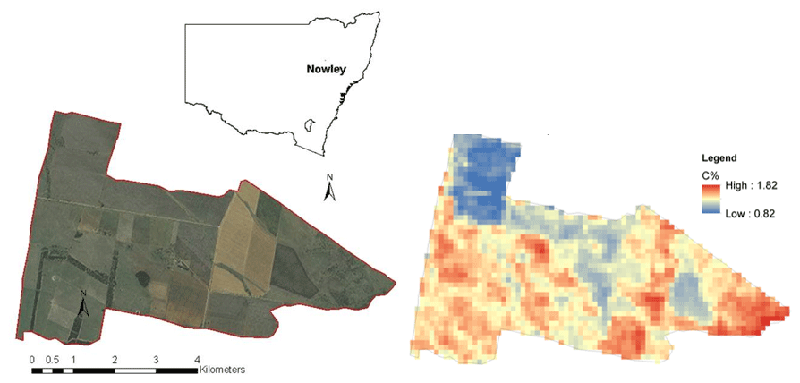
Figure 1The study area (left; sources: Esri, DigitalGlobe, GeoEye, i-cubed, USDA-FSA, USGS, AEX, Getmapping, AeroGRID, IGN, IGP, Swisstopo, and the GIS user community) and the coarse-scale topsoil soil organic carbon map (right).
3.1 Study area and coarse-scale soil carbon map
We illustrate the methodology by disaggregating a regional topsoil organic carbon map of the University of Sydney E.J. Holtsbaum Agricultural Research Station (Fig. 1). The landholding, also known as “Nowley”, is in the Spring Ridge district of the central/northwestern slopes of New South Wales (NSW), Australia. Its area is approximately 2300 ha and is managed as a mixed farming enterprise of cattle grazing throughout the year and wheat, barley, and canola in winter and sorghum and sunflower in the summer. Cropping is performed on soils derived from basalt parent materials. The average annual rainfall is 600 mm.
The available map is a NSW topsoil carbon map, which was generated using a local regression kriging technique (Somarathna et al., 2016). These maps are analogues of the nationally available soil carbon maps of Australia, which are available in separate layers corresponding to the depth intervals definition in the GlobalSoilMap product specifications (Arrouays et al., 2014). The standard soil depth layers are 0–5, 5–15, 15–30, 30–60, and 60–100 cm.
This NSW soil carbon map has a grid spacing of 100 m × 100 m, with block support of the same size. Hence, the map spatial resolution and the support are equal, which in turn means that the pixel values that make up the map represent a predicted mean for the area of each pixel. Commonly, the pixel values of a digital soil map are on point support, with the pixel value representing the value at a point that is usually at the centre of each pixel (Malone et al., 2013). Therefore, block kriging was used convert the maps to point-supported maps before the analysis.
The topsoil of the study area was represented by the depth interval of 0–7.5 cm, as this was the depth interval used in previous work conducted at this site for soil carbon auditing (de Gruijter et al., 2016). The respective coarse (NSW) map for the 0–7.5 cm depth interval was predicted by using mass-preserving splines (Malone et al., 2009) of the 0–5 and 5–15 cm standardised maps. This map will hereafter be referred to as the coarse-scale map. It is this map that subsequent descriptions of spatial downscaling will refer to. The experimental variogram of the block-supported coarse-scale map is given in Fig. 2.
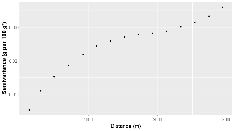
Figure 2Block support experimental variogram of the coarse-scale (100 m resolution) soil carbon map.
3.2 Environmental covariates
Elevation, topographic wetness index (TWI), gamma radiometric thorium, gamma radiometric potassium, Landsat band 4, and Landsat band 7 were used as environmental covariates in the spatial downscaling model. Landsat data have a resolution of 30 m. Since the coarse map was disaggregated into a 10 m resolution, the Landsat data were pan sharpened using the panchromatic band (15 m) and then resampled to 10 m.
The elevation data had been collected during a ground survey using an all-terrain vehicle with a 20 m swath. Then the data were processed using a local block kriging approach to produce elevation data at a 10 m resolution. Based on the developed digital elevation model (DEM), the TWI was derived. The gamma radiometric data were derived from aerial surveys (Minty et al., 2009), which were resampled to 10 m. A more detailed description of data collection and post-processing can be found in Malone et al. (2017).
3.3 Model parameter inferencing using the MCMC simulation
Suppose our observed soil carbon data (S) follows a second-order stationary Gaussian process which is characterised by the mean (trend) and the variogram where and where is a function of Euclidian distance h and θ vector of parameters of Matérn variogram (Eq. 14). The block averages SB have the same spatial mean as Sp but a different spatial structure (Gotway and Young, 2002). The block support covariance CBB is also a function of h, with a parameter vector of θ, but has a different support.
where Cij is the covariance between observation i and j, h represents the separation distance between i and j, δij denotes the Kronecker delta (δij=1 if i=j and δij=0 when I≠j), c0+c1 signifies the sill variance, and Kv is the modified Bessel function of the second kind of order υ. Γ is the gamma function, r denotes the distance or range parameter and υ is the spatial smoothness. Calculating CBB requires discretisation, and it was done using a regular grid pattern, with equal 10 m spacing between discretising points within a block. Then CBB was calculated according to Eq. (11).
The priors were given as informative priors and considered as normally distributed. The coarse-scale soil carbon map was regressed against the selected covariates to estimate the approximate prior values for the coefficient of the linear trend (β). Gaussian priors were assigned for both the spatial trend (β) and covariance component (θ) of the spatial model. MCMC integration was carried out using the Metropolis–Hastings algorithm. Metropolis–Hastings is a computationally efficient algorithm that allows sampling from conditional distributions (Diggle et al., 1998). Calibration of the model was done using two parallel chains of MCMC with 100 000 iterations.
3.4 Spatial prediction
The mean 95 % upper and lower CI limits of the spatial model parameters were calculated using the values of the last 10 000 MCMC iterations. These calibrated parameters were used to predict the SOC content at the fine scale. The predictions were made onto the 10 m × 10 m points based on Eq. (4).
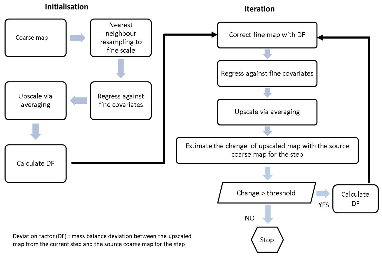
3.5 Disaggregation using dissever
The proposed Bayesian model was also compared with the dissever regression-based disaggregation approach. Dissever is a regression-based downscaling approach proposed by Malone et al. (2012). Dissever operates in two steps, namely initialisation and iteration. At the initialisation step, the coarse map is resampled using the nearest neighbour resampling technique to match the resolution of available fine-scale covariates. Then the resampled map is regressed against the fine-scale covariates. Next, the regressed fine map is upscaled through averaging, and then the mass balance deviation (deviation factor – DF) from the coarse map is calculated. The regressed fine map is corrected using the DF, and then the algorithm progresses to the iteration step. In the iteration step, regression and upscaling continue until the mass balance deviation between the upscaled map and the original map is less than a set minimum (threshold). The following flow diagram (Fig. 3) is an illustrative description of the dissever algorithm. This differs from Bayesian ATPRK since it is not focused on addressing the change in support problem, and it is a fine-gridding exercise. A detailed and comprehensive account of dissever can be found in Malone et al. (2012; 2017).
Following the procedure mentioned above, the coarse-scale carbon map of the area was disaggregated into 10 m using dissever. The environmental covariates used in the Bayesian approach were similarly made available for dissever.
3.6 Independent validation
3.6.1 Validation data
The accuracy of the model was tested using an independent dataset, which consists of 127 soil samples from 0–7.5 cm soil cores (cross section area of 41 cm2 and height of 7.5 cm). The samples are considered to have point support. These data were collected over two separate soil surveys during 2014 and 2015, using stratified random sampling. Stratification was based on the SOC prediction fields generated from digital soil mapping. A detailed description about the stratified random sampling process can be found in de Gruijter et al. (2015). The carbon content of the collected soil cores was measured using dry combustion by an Elementar Vario Max CNS macro elemental analyser (Elementar Analysensysteme GmbH, Langenselbold, Germany). The measured carbon contents are in carbon concentrations (g of C per 100 g of soil).
3.6.2 Validation statistics
The model accuracy was compared using mean squared error (MSE) and Lin's concordance correlation coefficient (CCC; Lin, 1989) between the disaggregated values and observed independent values at sampling points.
CCC is given by the following:
where ρ is the correlation coefficient, σx,σy are the variances of observed (x) and predicted (y) values, and μx,μy are the respective means. CCC is scaled between −1 and 1, with the latter implying perfect agreement and the former implying perfect reverse agreement.
MSE is given by the following:
where Sp is the observed values of SOC at independent sampling points, is predicted SOC values at the fine scale, and n′ is the number of independent SOC samples at a fine scale. MSE is an indication of the accuracy of predictions, while CCC indicates both accuracy and precision of the disaggregation exercise.
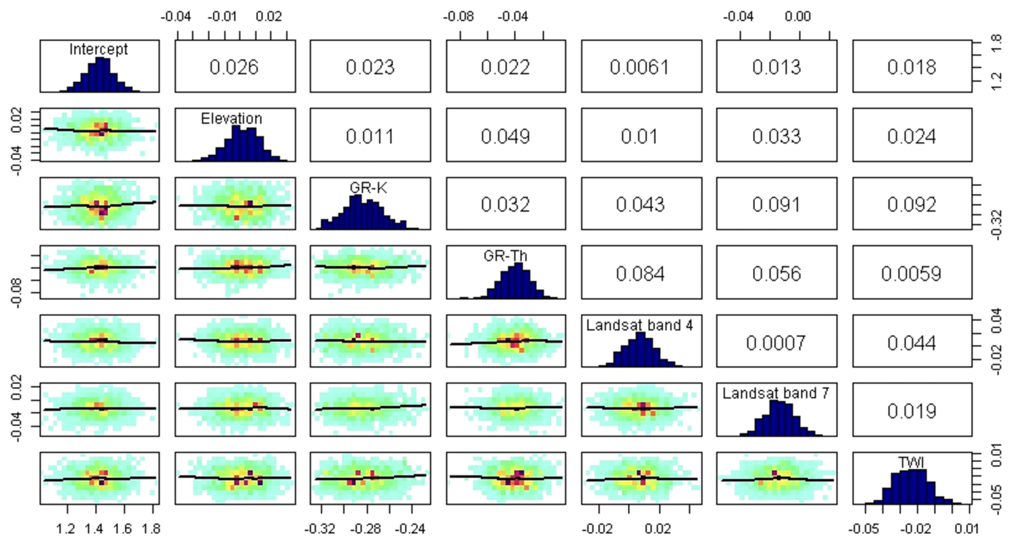
Figure 4Correlations and posterior distributions of linear trend parameters of the spatial model.
Table 11. Posterior parameters of the linear trend model.
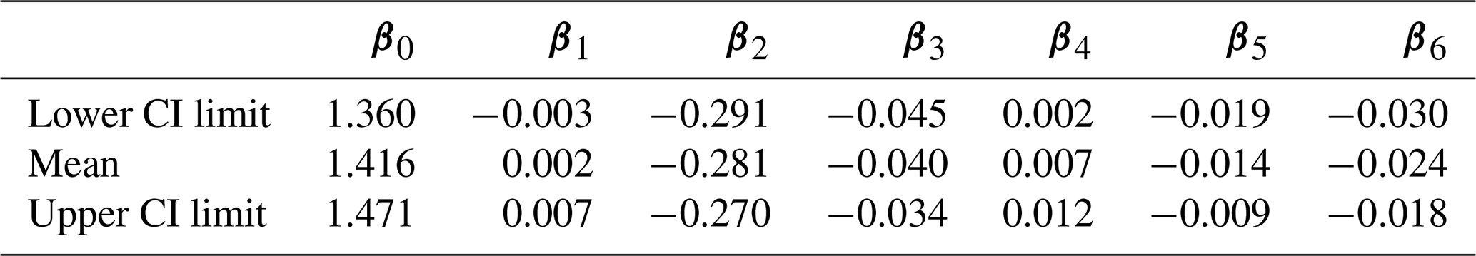
β0, β1, β2, β3, β4, β5, and β6 are the coefficients of the linear trend for intercept, elevation, TWI, gamma radiometric thorium, gamma radiometric potassium, and Landsat band 4 and Landsat band 7 parameters, respectively.
The use of the linear mixed model (LMM) as the spatial prediction model allows integration of fine-scale covariate information and spatial correlation in a single model. Unlike regression kriging in which regression and residual kriging are used in two phases of modelling, LMM is a one-step process. We used Bayesian inference techniques to estimate the parameters of LMM to deliver uncertainty estimates of the model parameters. This section provides a description of the posterior parameters of the spatial model followed by a comparison of spatially disaggregated maps using Bayesian ATPRK and dissever.
4.1 Bayesian parameter estimation of the spatial model
Figure 4 illustrates the posterior statistics of the linear trend parameters. The upper diagonal panel displays the correlation coefficients among the covariates, the lower diagonal depicts the scatter plots, while the diagonal shows the posterior distributions. The diagonal histograms are well defined, which indicates that all parameters of the linear trend are relatively well defined. The correlations among covariates are minimal, which indicates that there is no multicollinearity between the covariates.
Figure 5 displays the posterior distribution of Matérn variogram parameters and their correlations. Posterior values of the range parameter are similar to the prior values. However, the partial sill and nugget parameters are different from their priors. The posterior partial sill is higher than the prior sill, which agrees with the fact that the coarse-scale variability of soil carbon is lower compared to the finer scale (Fig. 5b).
Tables 1 and 2 provide the estimates of the parameters of the spatial model along with the 95 % confidence limits, which is an indication of the uncertainty of the parameters. The estimated posterior parameters have narrow CI limits, indicating the estimated mean provides a good approximation of the soil carbon content of the study area.
4.2 Spatial disaggregation using Bayesian ATPRK
Figure 6 displays the Bayesian ATPRK disaggregated soil carbon content of Nowley at 10 m, along with the 95 % confidence interval limits. Unlike other methods which only give a single estimate of mean soil carbon content, the Bayesian technique provides a range and/or interval of the most probable value with a 95 % confidence. These estimates are more reliable as they are generated using numerous repeated samplings. Accuracy and confidence in estimates are important parameters for planning, designing, and implementing soil management. Therefore, Bayesian ATPRK provides a comprehensive output of soil carbon estimates at the farm scale.

Figure 5(a) Correlations and posterior distributions of variogram parameters (b) and the point and block support variograms.
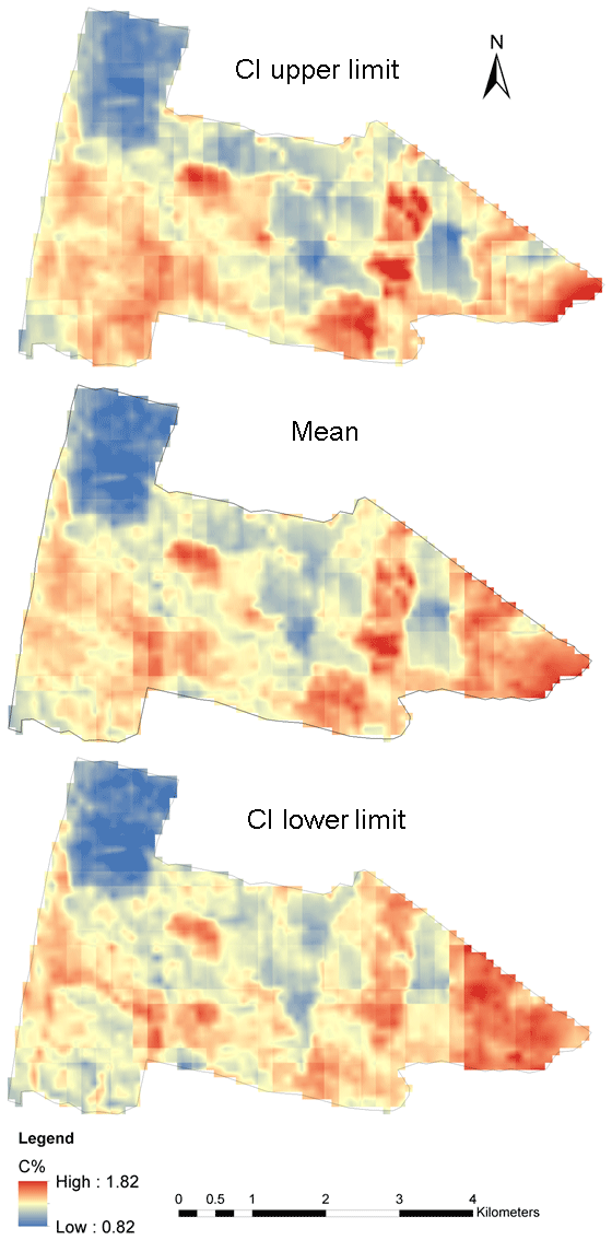
Figure 6Bayesian ATPRK disaggregated map with 95 % confidence limits.
4.3 Comparison of Bayesian ATPRK and dissever disaggregation methods
The disaggregated maps from both techniques were upscaled using a spatial overlay to assess the accuracy of disaggregation. CCC values were calculated for both techniques. Figure 7 shows the agreement between the cell values of the coarse map and the upscaled disaggregated maps.
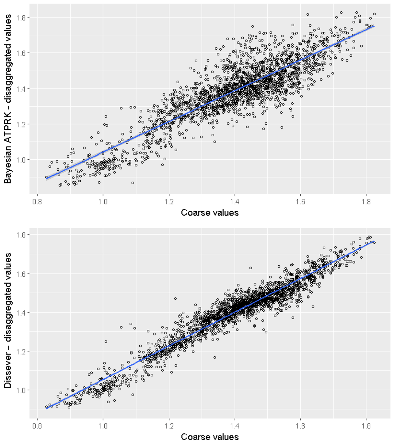
Figure 7Correlation plots between upscaled disaggregated values from Bayesian ATPRK, dissever, and original coarse-scale block values.
Concordance correlation between the original coarse values and upscaled product were 87 % and 96 % for Bayesian ATPRK and dissever, respectively. Dissever iterates until the agreement between upscaled and original coarse cell reaches a set minimum, while Bayesian ATPRK output is a result of one simulation considering both the correlation with the covariates and covariance structure of the residuals. This explains the stronger concordance associated with dissever.
Figure 8 illustrates the comparison between the dissever and Bayesian ATPRK disaggregated product with the coarse-scale source map. A closer examination reveals that Bayesian ATPRK product resembles the spatial pattern of SOC more closely than the dissever product, while dissever seemingly over-predicts the SOC content.
Table 2Posterior parameters of the point support Matérn variogram model. CI refers to the confidence interval.
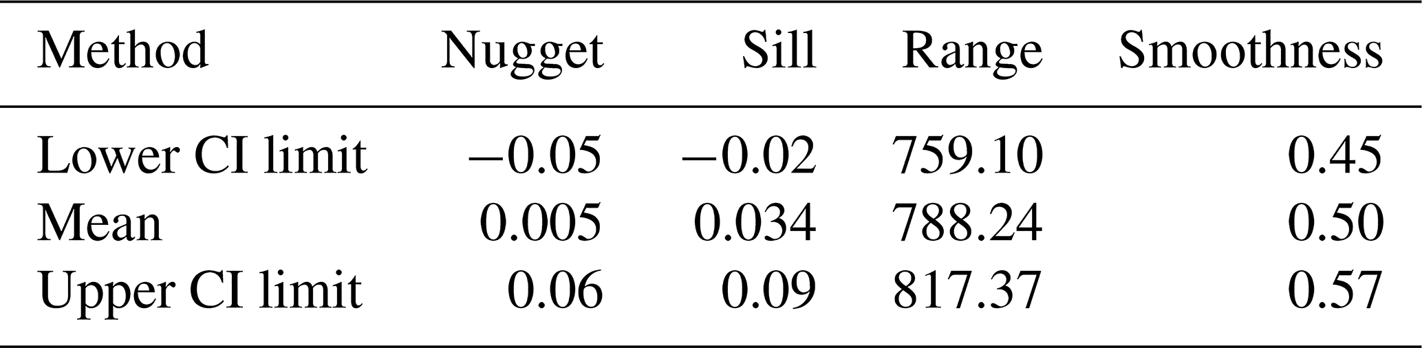
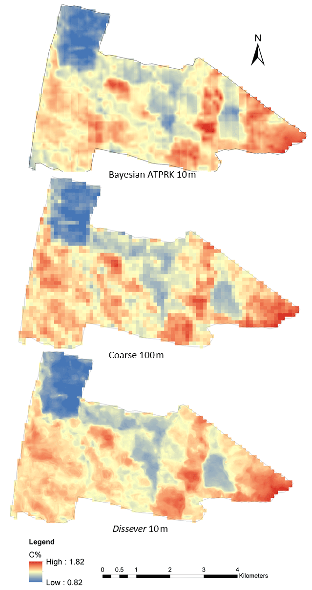
Figure 8Comparing the disaggregated map with original coarse-scale SOC map.
Conversely, dissever is computationally more efficient compared to Bayesian ATPRK. Calculating the block-to-point and block-to-block distance matrixes is a computationally expensive procedure. The whole study area cannot be computed in a single run using a desktop computer. Therefore, the study area has to be split into tiles, and predictions were carried out for each of the tiles. This resulted in abrupt changes between two tiles in the Bayesian ATPRK disaggregated map.
4.4 Validation of disaggregated maps
Independent validation results between disaggregated maps using dissever and Bayesian ATPRK indicate that Bayesian ATPRK technique is slightly more accurate compared to dissever-produced output in general.
The CCC value of Bayesian ATPRK was 23 %, while that of dissever was 18 %. Greater CCC indicates more accurate and precise predictions. The mean squared error (MSE %) of the Bayesian ATPRK product was 0.45 while MSE for dissever was 0.49, which indicates that Bayesian ATPRK disaggregation is slightly more accurate than dissever disaggregation.
Although the validation CCC is low, it still is a sufficient approximation in terms of SOC as the SOC prediction accuracy generally remains low. The coarse map is a product of regression for the whole region, which also has a lower concordance correlation with the sampled data. Through the disaggregation process, the errors tend to propagate, widening the gap between the actual and predicted SOC content.
Overall, we have demonstrated using Bayesian ATPRK for downscaling coarse-scale rasters to more informative fine-scale rasters by using available fine-scale covariates. The study proves that Bayesian ATPRK provides more accurate results with uncertainty estimates of the disaggregation process. There are a few limitations to this study. Firstly, we did not deal with the uncertainty from all sources of measurement errors. The coarse-scale map always carries a certain degree of error and/or uncertainty. Also, there is an uncertainty associated with the splining of the maps. Both of these uncertainties can be treated as measurement errors and filtered by adding as a noise variance along the diagonal of the covariance matrix CBB. Another way of correcting the bias is to use the measured data in the spatial model to reflect the actual ground conditions. Malone et al. (2017) demonstrated that the inclusion of the ground observations improves the accuracy of the disaggregated maps. A further limitation of our method is that the disaggregated map produced from Bayesian ATPRK has a block effect due to the final map being a collection of tiles produced separately due to the high computing demands of the model. This tiling effect can be eliminated by using high-performing and parallel-computing solutions to generate the fine-scale image in one go. Also, low-ranking representations (Wikle, 2010) of the covariance can also be used as a possible solution to the computational burden of the process.
Furthermore, although we have used the proposed Bayesian ATPRK in the DSM domain, this method can also be used to downscale coarse-scale satellite data. Even though there is a wide range of fine-resolution satellite images available in the present context, there is still a scarcity of fine-resolution data for certain parts of the world. Spatial downscaling is a solution to this data sparsity. There is a range of disaggregation and/or pan-sharpening techniques available in the literature. However, very few techniques can tackle the uncertainty of source images and the uncertainty of the disaggregation process. Unlike other methods, Bayesian ATPRK can explicitly help to tackle observation errors of the satellite images.
The study demonstrates that Bayesian techniques can be effectively used to address the change in the support problems. Monte Carlo integration provides the estimates of point-supported covariance structures using block-supported data along with uncertainty estimates of the parameter inference. This study used informative priors of covariance parameters, as the soil carbon data were available for the study site. In the absence of prior information, priors can be given as non-informative priors.
Bayesian ATPRK provides an effective way of disaggregating coarse-scale SOC maps. The output of this study facilitates policy making and soil management activities by providing the maps with confidence limits, which lead to a wider understanding of the SOC content of the area. However, the method is computationally intensive, and the use of high-performing computing techniques is recommended for faster and smoother predictions.
Furthermore, the noise of coarse-scale observations can be filtered through incorporating the noise variance in the diagonal of CBB. The use of point data (if available) in the spatial model can improve the accuracy of the disaggregation. Finally, the use of both techniques is recommended for lower uncertainty and improved accuracy of the disaggregation process.
The maps of this study are available from the authors upon request.
SNSPD, BuM and BrM designed the method. BrM collected and analysed the soil samples. SNSPD analysed the data and wrote the manuscript with the inputs from BuM and BrM.
The authors declare that they have no conflict of interest.
The authors are grateful to Gerard Heuvelink, from the Wageningen University and Research, and Phuong Truong, from the University of Twente, for sharing the R code on area-to-point kriging and providing constructive insight to this paper. Also, the authors extend their thanks to the two anonymous reviewers who provided constructive comments for the further improvement of this paper.
This research has been supported by the Australian Department of Agriculture (grant no. 1194105-66). Budiman Minasny is a member of a consortium supported by Le Studium Loire Valley Institute for Advanced Studies through its Le Studium Research Consortium Programme.
This paper was edited by Bas van Wesemael and reviewed by two anonymous referees.
Akpa, S., Odeh, I., Bishop, T., Hartemink, A., and Amapu, I.: Total soil organic carbon and carbon sequestration potential in Nigeria, Geoderma, 271, 202-215, https://doi.org/10.1016/j.geoderma.2016.02.021, 2016.
Arrouays, D., McBratney, A. B., Minasny, B., Hempel, J. W., Heuvelink, G. B. M., MacMillan, R. A., Hartemink, A. E., Lagacherie, P., and McKenzie, N. J.: The GlobalSoilMap project specifications, Glob. Basis Glob. Spat. Soil Inf. Syst., Taylor & Francis Group, London, 9–12, 2014.
Brus, D., Orton, T., Walvoort, D., Reijneveld, J., and Oenema, O.: Disaggregation of soil testing data on organic matter by the summary statistics approach to area-to-point kriging, Geoderma, 226–227, 151–159, https://doi.org/10.1016/j.geoderma.2014.02.011, 2014.
Cheng, Q.: Modeling Local Scaling Properties for Multiscale Mapping, Vadose Zone J., 7, 525, https://doi.org/10.2136/vzj2007.0034, 2008.
Cressie, N.: Statistics for spatial data, Wiley, New York, 1991.
Cressie, N.: Statistics for spatial data, Wiley, Hoboken, NJ, 2011.
de Brogniez, D., Ballabio, C., Stevens, A., Jones, R., Montanarella, L., and van Wesemael, B.: A map of the topsoil organic carbon content of Europe generated by a generalized additive model, Eur. J. Soil Sci., 66, 121–134, https://doi.org/10.1111/ejss.12193, 2014.
De Gruijter, J. J., Minasny, B., and McBratney, A. B.: Optimizing stratification and allocation for design-based estimation of spatial means using predictions with error, J. Surv. Stat. Methodol., 3, 19–42, 2015.
de Gruijter, J., McBratney, A., Minasny, B., Wheeler, I., Malone, B., and Stockmann, U.: Farm-scale soil carbon auditing, Geoderma, 265, 120–130, https://doi.org/10.1016/j.geoderma.2015.11.010, 2016.
Diggle, P. J., Tawn, J. A., and Moyeed, R. A.: Model‐based geostatistics, J. R. Stat. Soc. Ser. C, 47, 299–350, 1998.
Draper, D.: Assessment and Propagation of Model Uncertainty, J. Roy. Stat. Soc. B Met., 57, 45–70, https://doi.org/10.1111/j.2517-6161.1995.tb02015.x, 1995.
Gelfand, A.: On the change of support problem for spatio-temporal data, Biostatistics, 2, 31–45, https://doi.org/10.1093/biostatistics/2.1.31, 2001.
Goovaerts, P.: Kriging and semivariogram deconvolution in the presence of irregular geographical units, Math. Geosci., 40, 101–128, 2008.
Goovaerts, P.: A coherent geostatistical approach for combining choropleth map and field data in the spatial interpolation of soil properties, Eur. J. Soil Sci., 62, 371–380, 2011.
Gotway, C. A. and Young, L. J.: Combining incompatible spatial data, J. Am. Stat. Assoc., 97, 632–648, 2002.
Gotway, C. A. and Young, L. J.: A geostatistical approach to linking geographically aggregated data from different sources, J. Comput. Graph. Stat., 16, 115–135, 2007.
Grundy, M., Rossel, R. V, Searle, R., Wilson, P., Chen, C., and Gregory, L.: Soil and landscape grid of Australia, Soil Res., 53, 835–844, 2015.
Grunwald, S.: Multi-criteria characterization of recent digital soil mapping and modeling approaches, Geoderma, 152, 195–207, 2009.
Kerry, R., Goovaerts, P., Rawlins, B. G., and Marchant, B. P.: Disaggregation of legacy soil data using area to point kriging for mapping soil organic carbon at the regional scale, Geoderma, 170, 347–358, 2012.
Kyriakidis, P. C.: A geostatistical framework for area-to-point spatial interpolation, Geogr. Anal., 36, 259–289, 2004.
Lagacherie, P.: Digital Soil Mapping: A State of the Art, in: Digital Soil Mapping with Limited Data, edited by: Hartemink, A. E., McBratney, A., and de L. Mendonça-Santos, M., Springer Netherlands, Dordrecht, 3–14, 2008.
Lin, L. I.-K.: A Concordance Correlation Coefficient to Evaluate Reproducibility, Biometrics, 45, 255–268, 1989.
Liu, D. S. and Pu, R. L.: Downscaling thermal infrared radiance for subpixel land surface temperature retrieval, Sensors, 8, 2695–2706, 2008.
Malone, B. P., McBratney, A. B., Minasny, B., and Laslett, G. M.: Mapping continuous depth functions of soil carbon storage and available water capacity, Geoderma, 154, 138–152, 2009.
Malone, B. P., McBratney, A. B., and Minasny, B.: Spatial scaling for digital soil mapping, Soil Sci. Soc. Am. J., 77, 890–902, 2013.
Malone, B. P., Styc, Q., Minasny, B., and McBratney, A. B.: Digital soil mapping of soil carbon at the farm scale: A spatial downscaling approach in consideration of measured and uncertain data, Geoderma, 290, 91–99, 2017.
McBratney, A. B., Santos, M. L. M., and Minasny, B.: On digital soil mapping, Geoderma, 117, 3–52, 2003.
Minasny, B., McBratney, A. B., and Part, B.: Digital soil mapping: A brief history and some lessons, Geoderma, 264, 301–311, 2016.
Minty, B., Franklin, R., Milligan, P., Richardson, M., and Wilford, J.: The radiometric map of Australia, Explor. Geophys., 40, 325–333, 2009.
Mulder, V. L., Lacoste, M., Richer-de-Forges, A. C., and Arrouays, D.: GlobalSoilMap France: High-resolution spatial modelling the soils of France up to two meter depth, Sci. Total Environ., 573, 1352–1369, 2016.
Nagle, N. N., Sweeney, S. H., and Kyriakidis, P. C.: A Geostatistical Linear Regression Model for Small Area Data, Geogr. Anal., 43, 38–60, 2011.
Odgers, N. P., Sun, W., McBratney, A. B., Minasny, B., and Clifford, D.: Disaggregating and harmonising soil map units through resampled classification trees, Geoderma, 214, 91–100, 2014.
Pardo-Igúzquiza, E. and Atkinson, P. M.: Modelling the semivariograms and cross-semivariograms required in downscaling cokriging by numerical convolution–deconvolution, Comput. Geosci., 33, 1273–1284, https://doi.org/10.1016/j.cageo.2007.05.004, 2007.
Reid, A., Ramos, F., and Sukkarieh, S.: Bayesian Fusion for Multi-Modal Aerial Images, in: Proceedings of robotics: science and systems, Berlin, Germany, Cambridge, MA: MIT Press, 1–8, 2013.
Román Dobarco, M., Orton, T. G., Arrouays, D., Lemercier, B., Paroissien, J.-B., Walter, C., and Saby, N. P. A.: Prediction of soil texture using descriptive statistics and area-to-point kriging in Region Centre (France), Geoderma Regional, 7, 279–292, 2016.
Roudier, P., Malone, B. P., Hedley, C. B., Minasny, B., and McBratney, A. B.: Comparison of regression methods for spatial downscaling of soil organic carbon stocks maps, Comput. Electron. Agr., 142, 91–100, https://doi.org/10.1016/j.compag.2017.08.021, 2017.
Somarathna, P. D. S. N., Malone, B. P., and Minasny, B.: Mapping soil organic carbon content over New South Wales, Australia using local regression kriging, Geoderma Regional Journal, 7, 38–48, https://doi.org/10.1016/j.geodrs.2015.12.002, 2016.
Truong, P. N., Heuvelink, G. B. M., and Pebesma, E.: Bayesian area-to-point kriging using expert knowledge as informative priors, Int. J. Appl. Earth Obs., 30, 128–138, https://doi.org/10.1016/j.jag.2014.01.019, 2014.
Wang, Q., Shi, W., Atkinson, P. M., and Zhao, Y.: Downscaling MODIS images with area-to-point regression kriging, Remote Sens. Environ., 166, 191–204, https://doi.org/10.1016/j.rse.2015.06.003, 2015.
Wikle, C. K.: Low-rank representations for spatial processes, in: Handbook of spatial statistics, edited by: Gelfand, A. E., Diggle, P. J., Fuentes, M., and Guttorp, P., 114–125, CRC Press, Chapman & Hall/CRC, Boca Raton, 2010.