Soil degradation assessment across tropical grassland of Western Kenya

Soils across sub-Saharan Africa are exposed to extensive degradation processes, which can reduce their ability to produce crops and support livestock. While there has been a significant research effort focussing on soil degradation in sub-Saharan croplands, less research effort had been directed towards grasslands. Here, we tested the effectiveness of remote sensing to classify the soil degradation status of smallholder grazing lands. Focussing on grasslands used by smallholders in the districts of Nyando and Kuresoi in Western Kenya, we first used remote sensing (RS) to classify grasslands as productive grazing lands, grazing lands that followed a variable trend in vegetation productivity (transition), and unstable and unproductive (degraded) grazing lands. We then tested how this classification related to measured soil parameters indicative of soil degradation. We then used this classification, which was based on a temporal analysis of Normalised Difference Vegetation Index (NDVI), Enhanced Vegetation Index (EVI) and Normalised Difference Water Index (NDWI) between 2013 and 2018, to identify 90 field sites across the two districts, which we then sampled and analysed for a range of physical, chemical and biological soil properties. Only soil microbial biomass carbon (C) showed consistent alignment with the RS classification, although there was some overlap with other soil parameters at one or other of the study areas. To group the sites using the soil variables, which we split by study area and into stable (those that are slow to change) and transient (those that change rapidly in response to a changing pedological environment), K-means clustering was undertaken. Two sets of clusters were produced for each district for the stable and transient variables. For the stable variables, at Kuresoi one of these clusters included sites with higher levels of C, nitrogen (N), phosphorus (P) and pH, that aligned well with the RS classification, with seven out of 10 productive sites being assigned to this cluster. At Nyando one of the stable variable clusters included sites with high soil C and N, but low pH and relatively low soil bulk density, and corresponded to 12 out of the 16 productive sites. For the transient variables, agreement between the clusters and the remote sensing classification was poor indicating a lack of utility for degradation assessment. Overall, our results suggest that while the use of RS methods for classifying degraded grasslands and the soils supporting them does have significant advantages in terms of time and costs over field survey, supplementing these methods with a limited set of soil parameters related to nutrient cycling, such as microbial biomass C, soil P, percent C and N, and soil pH, could enhance our ability to identify degraded soils and target restoration efforts.

1 Introduction

Approximately 660 million hectares of sub-Saharan African (SSA) soils are estimated to be degraded, which represents a significant portion of the global extent of degraded soils (Gibbs and Salmon, 2015). Soil degradation reduces the functioning of soils and is a result of multiple processes including soil erosion by wind, water and tillage, salinisation, nutrient depletion, and compaction (Bridges and Oldeman, 1999) and may be triggered by shifts in land use, management or climatic changes. Most attention has been placed on the impacts of soil degradation on food security, and it has been cited as the leading cause of stagnation in food production, creating uncertainties for income and nutritional security for rural populations (Barbier and Hochard, 2016). Reduced plant productivity associated with degraded soil also reduces the input of carbon (C) to the soil leading to lower C stocks (Bai and Cotrufo, 2022) and less biomass to support livestock. Further, when grazing lands are degraded, farmers are often forced to graze their livestock in adjacent forests, which can negatively affect forest plant communities (Mullah et al., 2023). Thus, restoring degraded soils has become a priority for securing future food supply while simultaneously avoiding biodiversity and C losses. This has resulted in several initiatives supporting landscape restoration in Africa, notably the African forest restoration initiative (World Resources Institute, 2026), which gathered commitments from African governments to restore 100 million ha of degraded land by 2030.

The East African highlands of Kenya are densely populated areas of high agro-ecological potential. Farms here are small, typically smaller than 2 ha (Lowder et al., 2016). Production includes a mix of grains and vegetables for local consumption, some cash crops, such as tea (Camellia sinensis (L.) O. Kuntze), and livestock keeping. Milk from livestock is important to smallholder families as a valuable source of protein in a protein-poor diet (Hulett et al., 2014). Grazing animals are also culturally significant, reflecting the social standing of the owner and providing meat for celebrations and an additional source of cash when sold (Moll, 2005). Smallholder systems in the highlands of Kenya have a range of stocking rates, typically expressed in Tropical Livestock Units (TLU) per hectare. Stocking rates in the Kenyan highlands are reported to be between 1 and 1.4 TLU ha⁻¹ depending on the nature of the system (Bebe et al., 2003), whereas for Murang'a County to the south east of our study area, they are 3–6 TLU ha⁻¹ (Ortiz-Gonzalo et al., 2017) and for dairy cattle in Kiambu County to the west of our study area an average of 2.1 TLU ha⁻¹ (Were et al., 2025). Additionally, grazing takes place on farms and on utility areas, which are controlled by local institutions; these often come under higher greater pressure because multiple livestock owners have access to the land. In response to these pressures, grassland soil degradation is widespread in Kenya (Nzau et al., 2018) although we know little about its extent and severity.

Given the importance of grazing land for sustaining rural livelihoods it is surprising that globally, and particularly in SSA, much less recent research attention has been placed on understanding degradation of grazing lands (Bardgett et al., 2021),. High grazing pressures can degrade soil fertility with associated declines in soil properties underpinning soil health (Pelster et al., 2017), for instance causing soil compaction and reducing soil infiltration rates (Owuor et al., 2018) and C inputs to soil due to the removal of plant material by livestock and reductions in root mass (Zhou et al., 2017). Further, catchments with high livestock densities have larger nutrient and sediment loads in streams (Jacobs et al., 2017), have greater emissions of greenhouse gases (Arias-Navarro et al., 2017), and increase the risk of forest degradation (Brandt et al., 2018). Low soil nutrient availability and the deterioration in soil physical properties impairs plant growth and alters plant nutrient concentrations (Augustine et al., 2003), and reduces organic matter return to soil. With poorer vegetation cover and lower organic matter contents, soils become increasingly vulnerable to erosion, leading to lower soil depth and organic matter, which further reduces water and nutrient retention (Quinton and Fiener, 2024). This leads to a downward spiral of productivity loss and reduced capacity of systems to resist and recover from climate extremes (Quinton and Fiener, 2024; van de Koppel et al., 1997).

The UN Decade (2021–2030) on ecosystem restoration (United Nations Environment Programme, 2019) has focused attention on understanding where and how severely soils are degraded and whether they can recover, which is clearly important for the design of restoration programmes. In grazed systems, soil degradation is often recognised by the presence of bare soil. However, using bare soil as an indicator can be problematic in systems where erratic rainfall patterns lead to seasonal and inter-annual fluctuations in vegetation growth coupled with reduced vegetation cover due to grazing (Ellis and Swift, 1988). In such environments, poor vegetation growth may or may not indicate degraded soils. However, utilising the response of vegetation to changed soil properties and water availability is an approach that has been used by several authors (e.g. Eckert et al., 2015; Zhou et al., 2017).

Here, we tested the reliability of remote sensing approaches for classifying degradation status of smallholder grazing land and compared it with an approach based on the sampling of soils and characterisation of soil properties related to soil structural stability and C, nitrogen (N) and phosphorus (P) cycling. Working in two areas representing smallholder grazing land of western Kenya (Nyando and Kuresoi), we assessed degradation using a dynamic multi-year approach to derive a range of metrics to quantify the magnitude, seasonality and interannual variability of the vegetation (Rufino et al., 2016), and then tested whether or not the classification was related to measured soil parameters. We then explored whether soil variables classified as either stable or transient could be used to classify soil degradation status in grasslands.

2 Methodology

2.1 Field areas

We used a comparative landscape-level analysis of two agro-ecosystems with different ecologies (Fig. 1). The study areas are in western Kenya covering the neighbouring basins of the rivers Sondu-Miriu and Nyando spanning land use transitions from East African montane forests to grasslands and croplands. Study area 1 (Kuresoi) is in Kericho county located in the Sondu river basin in the proximity of the Mau Forest, at an altitude ranging from 1688 to 2947 m a.s.l., a mean slope of 7.6° and a maximum of 29°, with an average rainfall of 1988±328 mm. The geology originates from the early Miocene, with phonolites dominating in the lower part of the catchment, and phonolitic nephelinites in the upper part. The topography is rolling with moderate slopes. A variety of Tertiary tuffs are found on the highest part of the Mau Escarpment (Jennings, 1971). Study area 2 is in Lower Nyando located in the Nyando river basin, with an average rainfall of 1150 mm and spanning from the foot of a plateau at 1781 towards Lake Victoria at 1170 m a.s.l., with a mean slope of 5.3° and with a maximum slope of 21 degrees. Topography is gently sloping, towards ephemeral and permanent drainage. Soils are derived from Holocene alluvial deposits, and a variety of parent materials including phonolites and granitic gneisses (IUSS, 2015). The Lower Nyando study area covers an area which is approximately 160 km², whilst the Kuresoi study area covers an area that is approximately 1300 km² next to the Mau Forest. More details on land use and vegetation are given below.

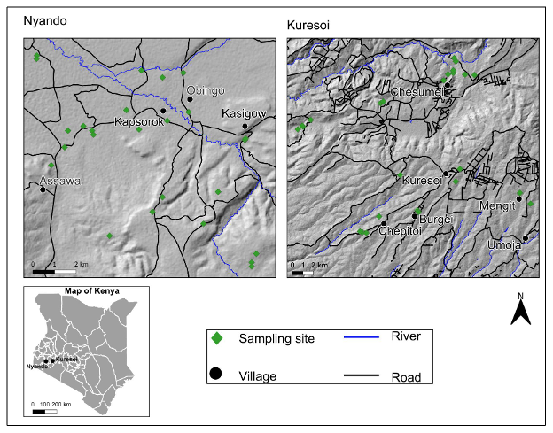
Figure 1 Location of study areas in Kenya (bottom left panel) and expanded views of Kuresoi (top right panel) and Lower Nyando (top left panel). Map produced using QGIS^® software. Road network, river and settlement were reproduced using OpenStreetMap vector data. Accessed on 9 June 2019 and are licensed under the Open Database 1.0 License. Digital Elevation Model was produced using ASTER Global Digital Elevation Model (GDEM) 30 m resolution as input and under license from NASA Earth Science Information Partners Data Preservation and Stewardship Committee 2019. Earth Science Data Ver. 2.

2.2 Approach to degradation classification

Our approach to classifying grasslands focusses on the rate at which greening takes place following a dry season (Yu et al., 2012). We define productive grasslands are those where biomass productivity is higher and returns rapidly following dry seasons. On the other hand, degraded grasslands are those with lower peak biomass and which display slow recovery following drought. Those grasslands that are intermediatory, displaying characteristics of both productive and degraded grasslands, are termed transition. These states are defined using an analytical approach using remote sensing images of both study areas which is set out in the following sections. This spatio-temporal analysis covered a period of 5 years (2013–2018).

2.3 Remote sensing data selection

To analyse the structural characteristics of grasslands supporting smallholder communities in Kuresoi and Lower Nyando, we implemented time-series seasonal analysis that classified landscape-level stages of degradation. We used 35 satellite image scenes from the archives of European Space Agency (ESA, 2016) and United States Geological Surveys (https://earthexplorer.usgs.gov/, last access: 20 April 2026) (Table 1). The selection of different sensors was necessary to: (i) fill missing dates from the Sentinel collection which had the higher spatial resolution, but shorter temporal resolution and (ii) to maintain consistency in annual seasonal sampling between 2013 and 2018. The final satellite imagery was from Landsat-Thematic Mapper (TM) L2, Landsat Operational Land Imager (OLI) L2 and Sentinel-2 sensors L2A. Level 2 images are Analysis Ready Data (ARD) and atmospherically corrected surface reflectance and data and therefore free from the effects of haze and water vapour. Landsat-TM and OLI imagery have a spatial resolution of 30 m, while Sentinel-2 imagery has a spatial resolution of 10 m.

Table 1 Summary of dates of acquisition of Landsat and Sentinel-2 imagery used for the determination of Normalized Difference Vegetation Index, Enhanced Vegetation Index and Normalized Difference Water Index.

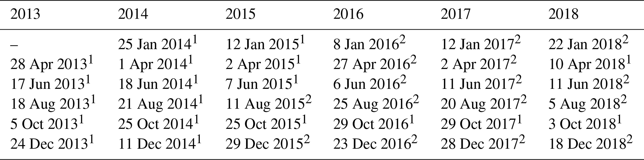
¹ Landsat Thematic Mapper (TM) or Operational Land Imager (OLI) imagery. ² Sentinel-2 imagery, Note: Landsat images were resampled to 10 m resolution.

The decision to select and process high-resolution imagery is due to the focus on smallholder dairy farms, which are associated with grazing lands that are often less than 1 ha and therefore easier to detect with higher resolution imagery. For LandSat-TM scenes, we downloaded blue (band 1), red (band 3), near-infrared (band 4), and shortwave infrared (band 6) spectral bands from USGS earth explorer repository. For Landsat-OLI scenes, we downloaded blue (band 2), red (band 4), near-infrared (band 5) and shortwave infrared (band 6). For the Sentinel-2 scenes, we downloaded blue (band 2), red (band 4), near infrared (band 8) and shortwave infrared (band 11). We loaded the individual bands into RStudio using the raster package (R. All Landsat images were resampled to 10 m using Sentinel-2 images as reference. This is because TIMESAT 3.3 (see description of use below), which is a program for analysing time-series of satellite derived index data by extracting seasonal parameters (Eklundh and Jönsson, 2015) and requires all input image scenes to have the same spatial resolution when creating raster stacks and before model fitting. No further image enhancements were applied because the TIMESAT algorithm reduces negative biases arising from cloudiness by fitting the model to the upper envelope of the vegetation/water index data (Eklundh and Jönsson, 2015). Despite these corrections, TIMESAT is unable to reduce negatively biased residuals related to surface anisotropy and sensor defects. However, we did not detect the effects of sensor defects in this analysis. Afterwards, we calculated NDVI values in each pixel by dividing the difference with the sum of near-infra red and red bands (Eq. 1). To derive EVI values in each pixel, we applied correction factors and divided the difference between near-infrared and red bands with near-infrared band (Eq. 2). We calculated NDWI in each pixel by dividing the difference with the sum of near-infrared and shortwave infrared (Eq. 3).

2.4 Temporal and seasonal analysis

Three vegetation indices, Normalised Difference Vegetation Index (NDVI), Enhanced Vegetation Index (EVI) and Normalised Difference Water Index (NDWI) were calculated using blue, red, near infra-red (NIR), and shortwave infra-red bands (Eqs. 1–3). These indices were selected because vegetation and water indices are effective to estimate changes in ecosystems (He et al., 2018) and grassland biomass (Todd et al., 1998), distinguish canopy density (Huete et al., 1997), and characterise drought (Rulinda et al., 2012).

$$\begin{array}{}\text{(1)}& {\displaystyle }& {\displaystyle }\mathrm{NDV}I={\displaystyle \frac{(\mathrm{NIR}-\mathrm{Red})}{(\mathrm{NIR}+\mathrm{Red})}}\text{(2)}& {\displaystyle }& {\displaystyle }\mathrm{EVI}=G\cdot \left[{\displaystyle \frac{(\mathrm{NIR}-\mathrm{Red})}{\left(\mathrm{NIR}+C_{\mathrm{1}}\cdot \mathrm{Red}-C_{\mathrm{2}}\cdot \mathrm{Blue}+L\right)}}\right]\text{(3)}& {\displaystyle }& {\displaystyle }\mathrm{NDWI}={\displaystyle \frac{(\mathrm{NIR}-\mathrm{SWIR})}{(\mathrm{NIR}+\mathrm{SWIR})}}\end{array}$$

where NIR is near-infra red; G represents a gain factor; L adjusts for canopy background; C₁ and C₂ are coefficients for atmospheric resistance (G=2.5, C₁=6, and C₂=7.5). Applying these coefficients allows for index calculation as a ratio between Red and NIR values, while reducing the background noise, atmospheric noise, and data saturation. Index values were calculated on a scale of −1 to 1.

The seasonality of the vegetation was interpolated using TIMESAT v3.3 algorithm (Eklundh and Jönsson, 2015). An adaptive Savitzky–Golay smoothed function was fitted over the index time-series data of Lower Nyando to model bi-modal seasons and to determine the timings of the growing seasons. A double gaussian function was fitted over the index time-series data of Kuresoi to model seasonal peaks where the vegetation dynamics is less variable. The adaptive function of TIMESAT modelled abrupt changes in vegetation effectively, which was often the case in the Lower Nyando landscape consisting of an intricate mosaic of land covers. A double logistic function allowed to isolate noise (e.g. caused by clouds) in Kuresoi data. To capture seasonal peaks, the functions were fitted to the upper envelope of the time-series following Eklundh and Jönsson (2015).

2.5 Degradation units' classification

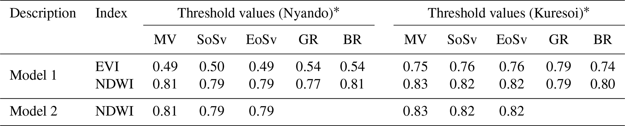
Five seasonal parameters were selected for the classification of degradation units: Start of Season (SoSv), Function value at End of Season (EoSv), Largest data, Maximum Value (MV), Greening rates (GR) and Browning rates (BR) because of the phenology characteristic of the ecosystems under study (Kong et al., 2022). For definitions of seasonal parameters and further explanations see Eklundh and Jönsson (2017). Productive vegetation state was expected to have higher values for SoSv, EoSv, MV and experience faster greening compared to vegetation of the units with transition and degraded states (Xiao et al., 2006; Yu et al., 2012). There are no predefined seasonal parameter values that define stages of grassland degradation in Western Kenya, as there are for other African grasslands (e.g. Tagesson et al., 2015 quantified maximum NDVI values between 0.59 and 0.82 for different grasslands in a semi-arid region of Senegal). Five models were tested and three were rejected as they could not differentiate between pasture and forest cover, leaving two models. The thresholds used for selected seasonal parameters for both models are given in Table 2. Thresholding was implemented using written functions in R (R Core Team, 2023) to partition parameter values into three groups corresponding to productive, transition, and degraded. All land cover types were retained during seasonal parameter estimation and classification to allow for accurate seasonal models of the study areas. Using the above approach and thresholds, productive vegetation was assigned to high MV (>0.8), high GR (>0.5), and low BR (<0.3). Vegetation at the degraded state had low MV (<0.5), low GR (≤0.8), and high BR (≥0.5) and transition grasslands were those falling between these values. Finally, the classification from each model was combined to determine areas of common agreement and produce maps identifying productive, transition, and degraded areas (Fig. 2). For Kuresoi, 49 % of all pixels were identically classified in model 1 and 2. This represented 6 330 389 pixels (or 633 km²) classified similarly as either productive, transient or degraded. In Nyando, 82 % of pixels were identically classified in model 1 and 2. Representing 1 329 048 pixels or (133 km²) of the landscape classified similarly as either productive, transient or degraded. Higher agreement in model classifications for Nyando might be due to a sharper contrast between degraded and live vegetation. Whereas in Kuresoi, the landscape is relatively heterogeneous and harder to separate transient from degraded pixels.

Table 2 Summary of models' description, seasonal parameters and threshold values used for degradation unit classification of Lower Nyando and Kuresoi.

2.6 Selecting sampling locations

Land cover data from the European Space Agency Climate Change Initiative land cover vector layer (ESA, 2016) was used to mask forests, urban and water bodies to detect grazing areas. Afterwards, locations were selected using the Fishnet tool of ArcGIS. Stratified random sampling was used to create sampling locations separated by a minimum distance of 1 km to select approximately 30 sampling locations for each degradation unit, resulting in 100 sampling locations including replacements. Locations land that coincided with recently cultivated areas (<10 years) and/or road tracks were removed following examination using Google Earth (2008–2018). Locations that had signs of recent cultivation or tillage lines were excluded. In October–November 2019, the locations were visited to remove sample locations that were inaccessible or when landowners denied access. In total, 90 sites were selected for study (Fig. 2).

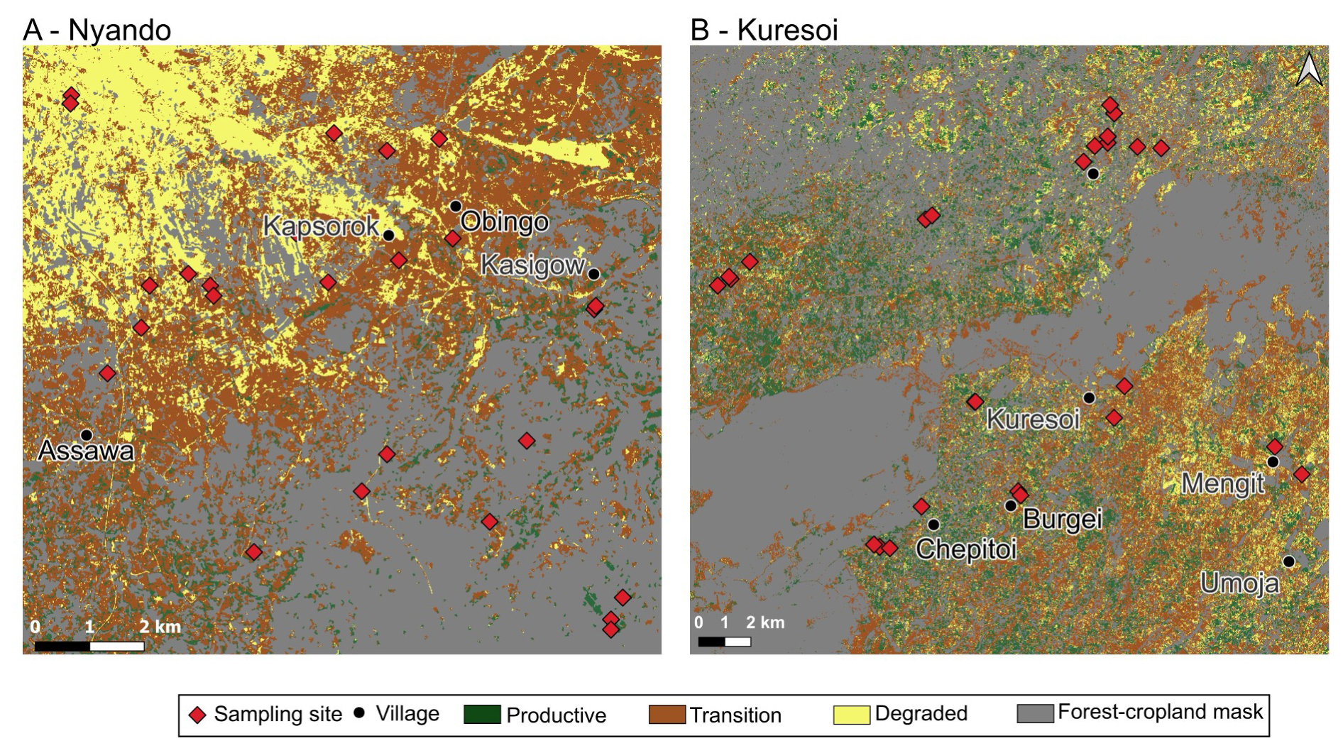
Figure 2 Classification of Lower Nyando (a) and Kuresoi (b) study areas into three units: productive, transition and regime-shift. Sampling sites are overlaid and show the distribution of field experiments and locations of soil and aboveground biomass samples. Map produced using QGIS^® software. Settlement information were reproduced using OpenStreetMap vector data. Accessed on 9 June 2019 and are licensed under the Open Database 1.0 License.

2.7 Soil sampling and analyses

Soils at each site were sampled to 10 cm depth and analysed for a range of physical, chemical and biological parameters (Table 3). For all analysis, unless stated, soils were air dried and ground to pass a 2 mm sieve prior to analysis.

Table 3 Mean and standard deviation (in brackets) of 28 soil variables (top 0–10 cm) by degradation labels measured at field sites in the two study areas, Kuresoi and Nyando, along with the significance level of the between label differences from ANOVA (where ^* represents p<0.1, and ${}^{**}$ represents p<0.05). Variables that show a significant difference between degradation classes at the p<0.1 level as determined by a pairwise t test are designated by a different letter in parenthesise.

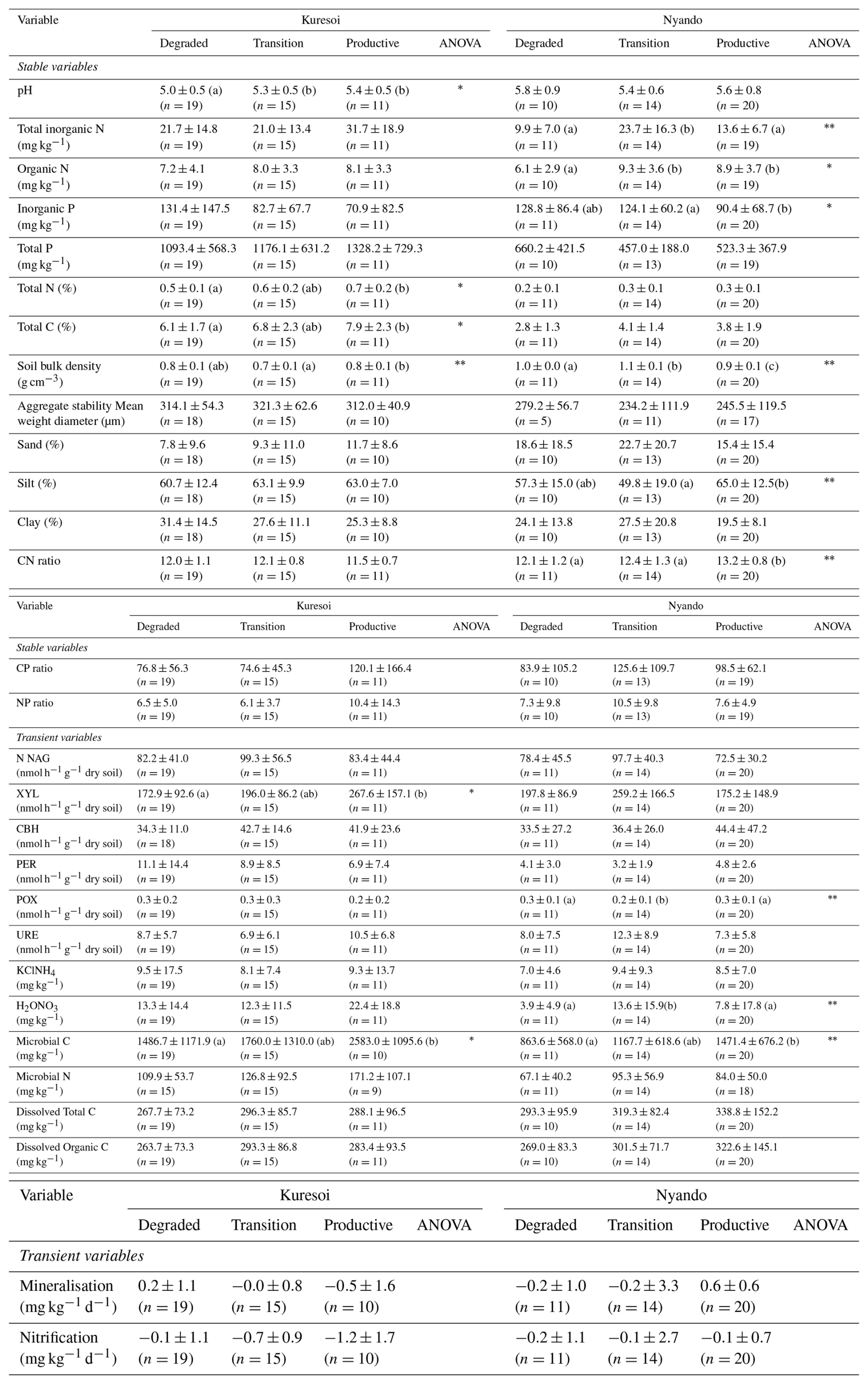
Bulk density was calculated following sampling of intact soil with 45 mm diameter rings. Soil texture was determined by laser diffraction (Beckman-Coulter LSI3 320), after soil dispersion in sodium hexametaphosphate. Aggregate stability was determined using the fast-wetting method of aggregate stability (Le Bissonnais, 1996), which subjects the aggregates to rapid immersion in water for 10 min. After that, aggregate samples were sieved in ethanol before oven drying to determine final aggregate size distribution, producing a mean weight diameter (MWD).

For each site sampled we measured total soil C, N, P, and selected microbial-mediated functions related to nutrient cycling. These were microbial biomass (C and N), nutrient availability (i.e. soluble inorganic and organic N and P pools, and dissolved organic C), rates of N mineralisation and nitrification. Briefly, percentage C and N in dry, ground soil were measured using an elemental combustion analyser (Elementar Vario EL, Hanau, Germany). We measured dissolved total and organic C (DC and DOC respectively), plant available nitrate (NO${}_{\mathrm{3}}^{-}$) and total dissolved N (TDN) by weighing 5 g of fresh soil accurately and shaking in 35 mL Milli-Q water for 10 min at 150 rpm, before filtering through Whatman 42 filter paper. C in the filtrate was quantified using an Aurora 1030W TOC analyser (OI Analytical, UK), and N was quantified using an autoanalyser (AA3, Seal Analytical, Wrexham, UK). Organic N was calculated by subtracting inorganic N values (nitrate and ammonium) from total N. pH of the filtrate was determined using a pH probe (Mettler Toledo FE20, Salford, UK). Values were adjusted for soil moisture. Soil ammonium (NH${}_{\mathrm{4}}^{+}$) was measured by shaking 5 g of fresh soil in 25 mL 1 M KCl for 30 min, extracting through Whatman 1 filter paper and analysing on the autoanalyser as before. For potential mineralisation and nitrification, 5 g of each soil sample was incubated for 14 d at 25 °C before being extracted and analysed for NH${}_{\mathrm{4}}^{+}$ and NO${}_{\mathrm{3}}^{-}$ using the KCl procedure. The values from the initial KCl extraction (summed NH${}_{\mathrm{4}}^{+}$ and NO${}_{\mathrm{3}}^{-}$) were subtracted from the day 14 extraction and divided by 14 to give a rate of potential mineralisation per day. Nitrification was calculated by using the NO${}_{\mathrm{3}}^{-}$ values only. Negative values imply denitrification, i.e. loss of N as N₂ gas. Microbial biomass C and N were determined using the chloroform-fumigation method (Vance et al., 1987). We weighed 5 g of each sample twice. The first replicates were shaken in 25 mL 0.5 M K₂SO₄ for 30 min, before passing through Whatman 42 filter paper. The second were placed in a desiccator containing a beaker of chloroform under vacuum for 24 h to lyse microbial cells, before being extracted as before. Total dissolved C and total extractable N were analysed using the Aurora and the autoanalyser respectively. Microbial biomass C and N were calculated by subtracting the unfumigated values from the fumigated ones. Total soil P was measured using the Kjeldahl digestion method (Kjeldahl, 1883). We mixed 420 mL concentrated sulfuric acid with 12 g lithium sulphate. We added 0.5 mL of this mixture to 50 mg of dry ground soil per sample in glass digestion tubes. We then added 0.5 mL 30 % hydrogen peroxide. Samples were heated at 200 °C, then we added a 50 °C heat increase every 30 min until it reached 360 °C. Samples were heated at 360 °C for 2 h before cooling. When cool, 0.5 mL of hydrogen peroxide was added and samples were digested at 360 °C for a further 2 h. Samples were diluted to 50 mL using Milli-Q water. They were analysed using the ascorbic acid microplate method after (Kuo, 1996), where samples were measured colourimetrically at 880 nm. For inorganic P, we placed 2 g of dry soil into a falcon tube with 50 mL of 0.5 M sulfuric acid. This was shaken at 150 rpm for 16 h. The samples were centrifuged at 1500 rpm for 10 min, and the supernatant was analysed using the ascorbic acid method (Olsen and Sommers, 1982).

In addition, a suite of extracellular enzyme activities involved in the degradation of cellulose, chitin, lignin and proteins – i.e. β-glucosidase (GLC), cellobiohydrolase (CBH), β-xylosidase (XYL), N-acetylglucosaminidase (NAG), phosphatase (PHO), phenol oxidase (POX), peroxidase (PER), and urease (URE) –, were determined which added artificial p-nitrophenyl (pNP) linked substrates to induce a colour reaction through p-nitrophenyl production following Broadbent et al. (2022).

2.8 Description of the data set

For testing and clustering analysis, we focused on a total of 28 soil variables measured from the soil samples collected from the 0–0.1 m depth in Kuresoi and Nyando. These variables were grouped in relation their rate of change in response to degradation as either stable (changes over multi-year time periods) or transient (changes over seasonal time periods) soil variables.

Bulk density and soil hydraulic properties change over multi-annual, timescales (Berisso et al., 2012), as can contents of C (Tully et al., 2015), N (Sun and Chen, 2025) and P along with pH (Tully et al., 2015), and thus were considered stable. Other soil physical variables (percentage sand, silt, and clay, and aggregate stability) were also considered stable. We reason that that as aggregate stability is strongly related to soil texture and organic matter (Kemper and Koch, 1966) both variables that change slowly, that aggregate stability will also change slowly, although there is little literature evidence to support this. In contrast, soil biological parameters, including enzyme activities, microbial biomass C, and rates of nutrient mineralisation, are expected respond rapidly to change in response to seasonal changes environmental conditions (Cordero et al., 2023) and therefore soil enzymes (PHO, GLC, NAG, XYL, CBH, PER, POX, URE), water extractable NO₃, and KCl-extracted NH₄, microbial biomass C, microbial biomass N, total dissolved C, organic dissolved C, mineralisation and nitrification were considered transient.

The statistical analysis for investigating the difference between degradation classes were carried out on the 28 variables across all 45 sites in Kuresoi and Nyando respectively. For the clustering analysis, the sites with incomplete data (i.e., with missing observation in any of the variables in the stable or transient variable sets) were removed, resulting in 31 sites in Nyando, 41 sites in Kuresoi for the stable variables, and 42 sites in Nyando, 38 sites in Kuresoi for the transient variables. The number of sites in each degradation class is given in Table 3.

2.9 Statistical analysis of field data

Statistical analyses were carried out to investigate differences in field sampling data between sites with different degradation labels allocated from remote sensing (Table 2). The analyses were applied to the data from Kuresoi and Nyando respectively. First, analysis of variance (ANOVA), with the soil variables being the response and the degradation class labels being the explanatory variable, was applied to soil variables which follow approximately a normal distribution, according to Shapiro–Wilks test. This is to identify any mean differences between the degradation classes. For variables that failed the normality test (i.e., having more than one degradation classes that are not normally distributed), the non-parametric Kruskal–Wallis test was used. For soil variables with a significant mean difference, further pairwise comparison tests were applied to each pair of degradation classes (i.e., productive vs. degraded, productive vs. transition, transition vs. degraded). Tukey's honest significant difference (HSD) test was used for parametric testing and Wilcoxon rank test was used for non-parametric testing.

2.10 Description of the clustering methods

Considering the features of our data sets, i.e., relatively large number of variables (12 and 16 for stable and transient variables respectively) as compared to the number of sites (between 31 to 42) in each area, relatively high variability in some variables, and initial experiments with different clustering methods, we chose to use k-means clustering for our main analysis. In particular, the k-means clustering was applied to the principal components extracted from the data. Below we briefly introduce the clustering method and provide some details on the approach we took.

K-means clustering is a popular method for grouping a population of n subjects (n being the number of sites in this case), each of p-dimensional (p being the number of covariates), into a number of k clusters, using algorithms developed by e.g. Hartigan and Wong (1979), Lloyd (1982), MacQueen (1967) and Fraley and Raftery (2002). Few assumptions are required for applying the k-means algorithm, although it has been acknowledged that the method works better with clusters that are of similar shapes or sizes (Steinley, 2006). The result can be sensitive to outliers (Johnson and Wichern, 2007). To determine the number of clusters for k-means clustering, methods such as elbow plot of the total sum of squared distance between points and cluster centres and gap statistics (Tibshirani et al., 2001) can be used (Scrucca et al., 2023), To begin with, principal component analysis (PCA) was applied to reduce the dimension of the data. The number of principal components (PCs) was selected to account for at least 80 % of the variation in the data. This resulted in six PCs each for the clustering of stable and transient variables from Kuresoi and Nyando respectively, which helped to improve the stability of the clustering algorithms. Due to the relatively small population size in this analysis, only cluster numbers from two to five were investigated. Based on the model selection criteria, after taking the robustness of the clustering results into account and discounting the cluster numbers that resulted in singletons (i.e., one site as a group of its own), the cluster number was settled to be two for both stable and transient soil variable sets in Kuresoi and Nyando.

The k-means clustering analysis was implemented in R (R Core Team, 2023) using the “mclust” package (Scrucca et al., 2023). Investigation of the clustering results was carried out in R using the “fossil” package (Vavrek, 2011).

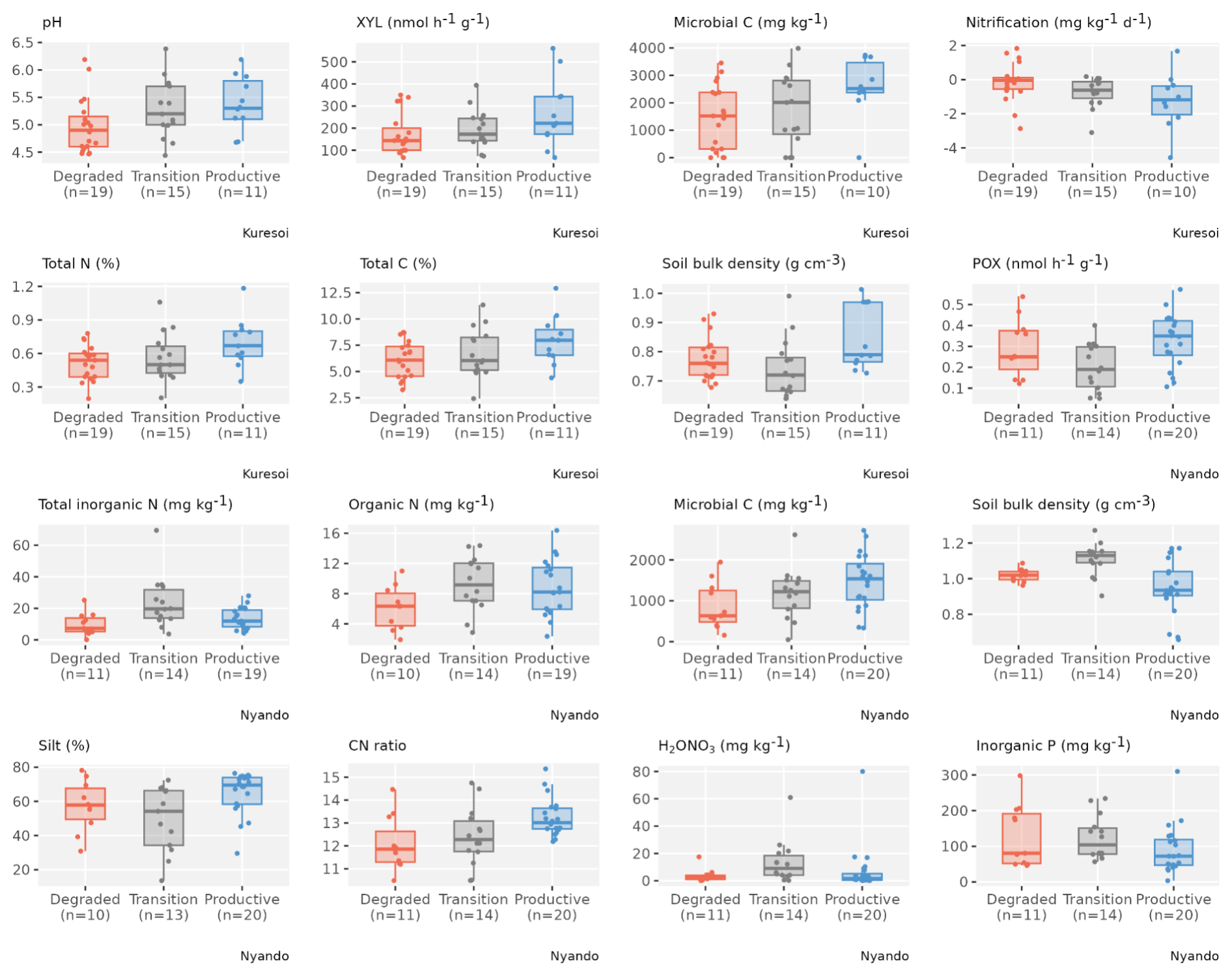
Figure 3 Box and whisker plots of the soil variables with significant difference between degradation classes based on ANOVA or Kruskal–Wallis test from Kuresoi and Nyando respectively. The coloured dots are observations overlaid on top of the box plots.

3 Results

3.1 Relation of remote sensing classification to measured soil parameters

Table 3 reports the mean and standard deviation for the soil variables measured in the two study areas and identifies those variables that showed significant differences between degradation states, which are then plotted in Fig. 3. Microbial biomass C and soil bulk density were the only two variables that showed significant differences (p<0.1) between degradation classes at both areas. There was a significant increase (p<0.05) of 74 % in mean microbial biomass C from degraded sites to productive sites at Kuresoi, and a significant increase (p<0.05) of 70 % at Nyando. Although the differences between the transition and degraded/productive sites were not significant, the rankings of the class means were consistent (degraded < transition < productive) for both areas. The largest difference in soil bulk density was seen between the transition class and the productive class for both Kuresoi (p<0.05) and Nyando (p<0.05). In this case, the rankings are inconsistent, with productive > degraded > transition at Kuresoi and transition > degraded > productive at Nyando, although the absolute differences between the classes were small (cf. 0.1 g cm³). Of the other soil variables that showed significant differences between degradation classes within each area: pH, total N and C and XYL at Kuresoi and C : N ratio at Nyando ranked the classes in the order degraded < transition < productive; inorganic P ranked the classes in the order of degraded > transition > productive, but the difference between degraded and transition is insignificant. Specifically, at Kuresoi, mean pH increased by 0.4 from the degraded to productive class, mean total C increased from 6.1 % to 7.9 %, mean total N from 0.5 % to 0.7 %, and mean XYL increased by 54 %, from 172.9 to 267.6 nmol h⁻¹ g⁻¹ dry soil. At Nyando, soil C : N ratio increased from 12.1 in the degraded class to 13.2 in the productive class.

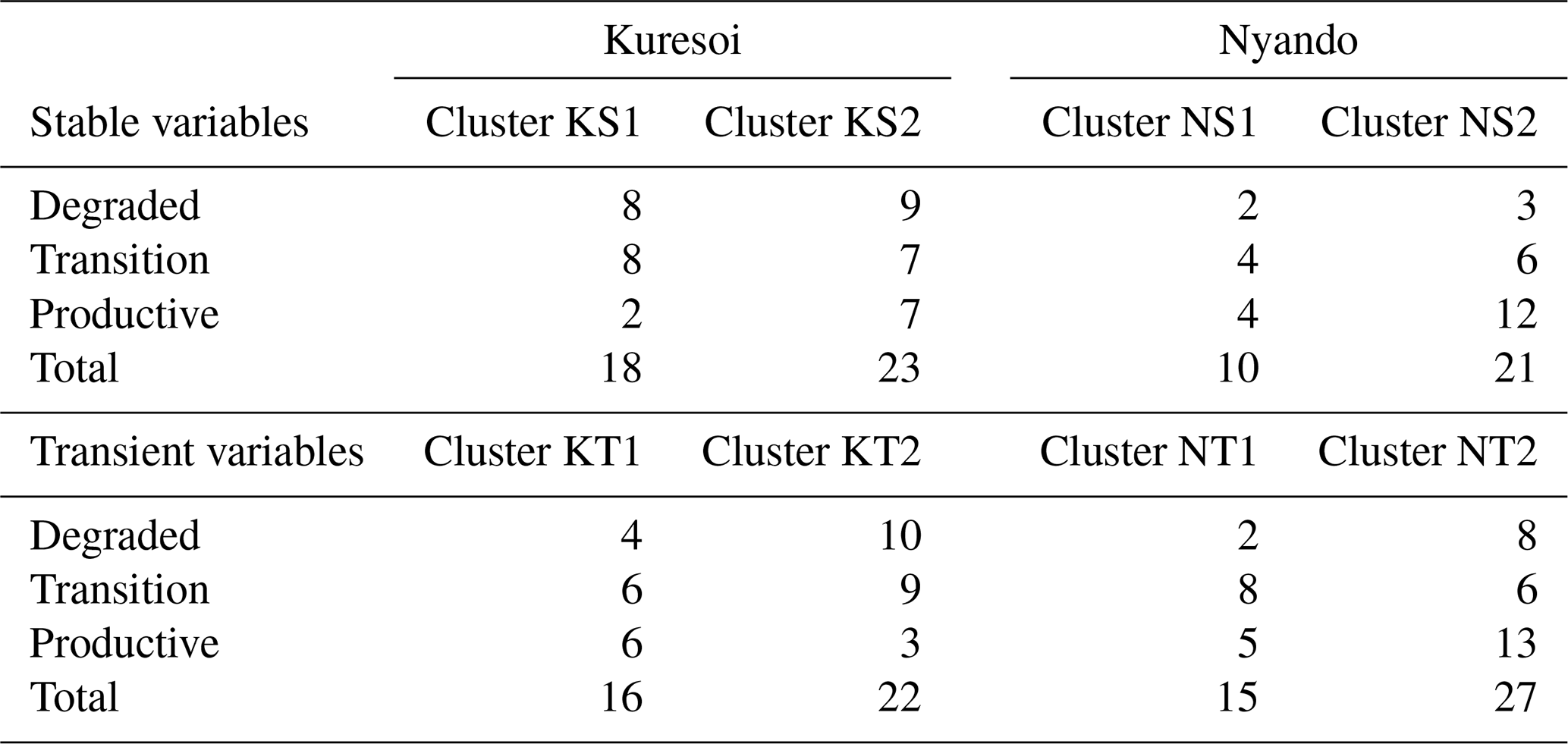
Table 4 Number of degraded, transition and productive sites allotted to stable (S) and transient (T) clusters at Kuresoi (K) and Nyando (N) using K-means clustering.

It should be noted that the productive class at Kuresoi and the degraded class at Nyando both have relatively small sample sizes (around 10 to 11 observations), which, given the relatively high coefficients of variation (i.e., the ratio between the standard deviation the mean of a variable), results in a low statistical power in the class mean difference test. The small sample size is expected to contribute to the insignificant differences between classes in some variables. We can reason that, had we had a larger sample size, that more variables may have shown a significant difference between the degradation classes. Therefore, the disagreement between the degradation classification based on the remote-sensing data and the soil sampling data does not necessarily negate the relationship between the two. Instead, it suggests that more field sampling data may be needed to reach a more conclusive result.

3.2 Which stable and transient soil variables explain the clustering of soils in the two study areas and do the clusters relate to degradation status?

Table 4 summarises the number of sites in Kuresoi and Nyando that have been grouped into two clusters by the k-means algorithm for stable and transient variables. Note that the total number of sites used in the clustering analysis for each area is different.

For the stable variables, in Kuresoi, sites in cluster KS2 had significantly higher values of total N, total inorganic N, organic N, total P, total C and pH (significant at 0.05 level under two-sample t tests). There was a significant difference in silt and clay contents of the two stable clusters. From Table 4, we see that 7 out of 9 Kuresoi productive sites, from the remote sensing classification, were assigned to cluster KS2, but the numbers of transitional and degraded sites were distributed evenly between two stable clusters. Similarly, in Nyando, one cluster (cluster NS2) had higher levels of total P, total N and total C, but lower pH and relatively low soil bulk density (all significant at p<0.05 level). There was a significant difference in sand, silt and clay percentages. In total, 12 out of 16 productive sites in Nyando were assigned to cluster NS2. The transitional and degraded sites appeared to be equally likely in two stable clusters.

For the transient variables, in Kuresoi, sites in one cluster (cluster KT1) tended to have higher PHO, GLC, XYL, CBH, but lower POX. It also had higher microbial N, nitrate (extracted in H₂O NO₃), microbial C, total dissolved C. In Nyando, one cluster (cluster NT1) consisted of sites with higher PHO, GLC, XYL, NAG, total dissolved C, but lower PER and POX. The cluster labels did not match the degradation labels in both cases. Box plots showing how the two clusters differed in selected stable (Fig. 4) and transient (Fig. 5) variables are given for Kuresoi and Nyando. All variables shown in the figures have significant mean difference at p<0.05 level under a two-sample t test.

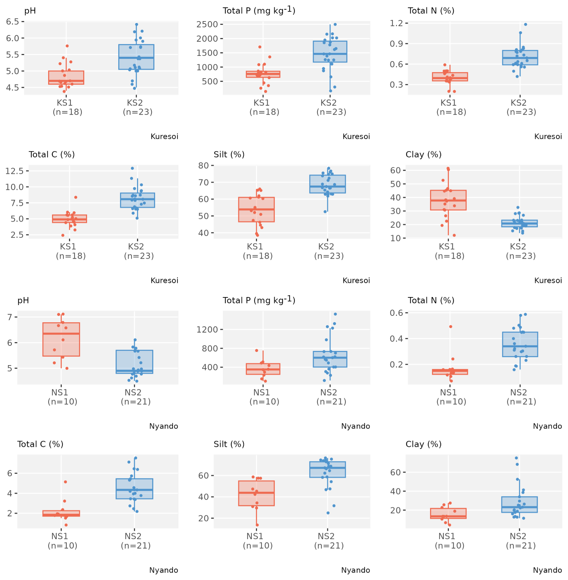
Figure 4 Box and whisker plots of selected stable variables that show a significant mean difference (p<0.05) between two clusters in both Kuresoi and Nyando, with observations (coloured dots) overlaid on top.

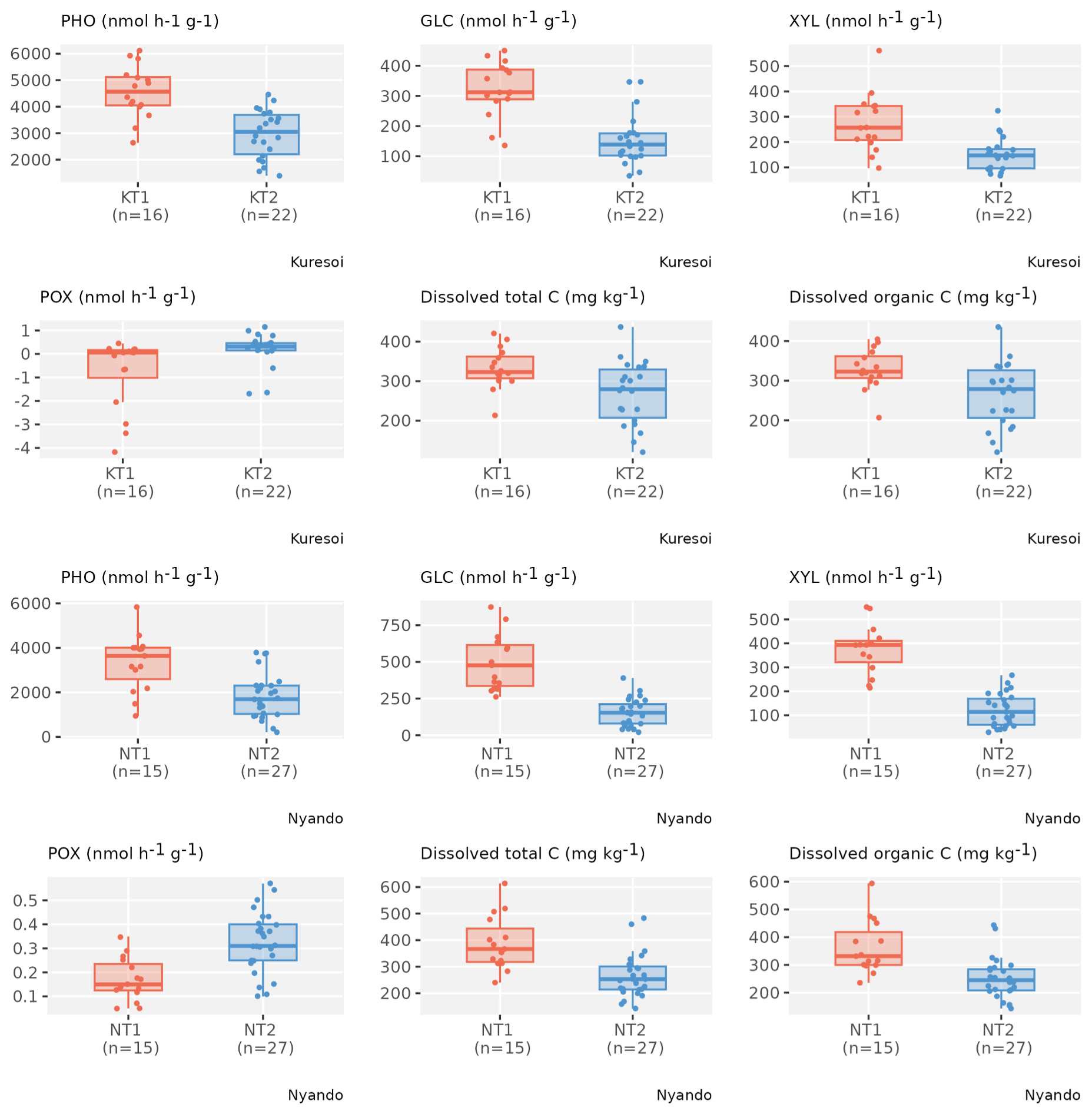
Figure 5 Box and whisker plots of selected transient variables that show a significant mean difference (p<0.05) between two clusters in both Kuresoi and Nyando, with observations (grey dots) overlaid on top.

To further investigate the features of the clusters, we evaluated the inter-quantile range (IQR) between the 0.15 and 0.85 quantiles of the samples from sites allocated to each cluster, representing the spread of about 70 % of the samples. For stable variables in Kuresoi, the IQRs of the samples from sites allocated to cluster KS1 are 401 to 1091 (mg kg⁻¹) for total P, 0.35 % to 0.50 % for total N, and 3.98 % and 5.76 % for total C. Whereas the IQRs of the sites allocated to cluster KS2 are 893 to 2024 (mg kg⁻¹) for total P, 0.56 % to 0.82 % for total N, and 6.55 % and 9.64 % for total C. In Nyando, the sites allocated to cluster NS1 have IQRs of 181 to 503 (mg kg⁻¹) for total P, 0.11 % to 0.21 % for total N and 1.58 % to 2.92 % for total C. The sites allocated to cluster NS2 have IQRs of 307 to 1226 (mg kg⁻¹) for total P, 0.23 % to 0.49 % for total N and 3.38 % to 6.38 % for total C. Overall, the clustering analysis grouped the sites with higher or lower total N and total C relatively well, with the IQRs show clear difference between two clusters. However, there are some overlaps between the IQRs of total P from two clusters for both Kuresoi and Nyando. For the transient variables, we see mostly overlapping IQRs between clusters, except for GLC in Kuresoi, and GL and XYL in Nyando.

4 Discussion

4.1 Relation of remote sensing classification to measured soil parameters

The ability of remote sensing to classify degradation status over large areas (e.g. Cordell et al., 2017; Manić et al., 2022; Wang et al., 2024), at relatively low cost and utilising data that can be rapidly updated as new images become available, is an attractive proposition, since it provides land managers, policy makers and scientists with a mechanism for targeting interventions. Combined remote sensing and measurement of soil properties has been used to map soils in Africa with some success (Vågen et al., 2016). Nevertheless, there have been relatively few attempts to compare remotely sensed classification against soil data collected from soil sampling programmes. Our work demonstrates that, while it is relatively straightforward to generate classifications using derived parameters, such as NDVI, NDWI and EVI, that reflect vegetation dynamics, the resulting classification only reflected changes in a few in-situ soil parameters related to soil degradation.

Across the two studied districts (i.e., Nyando and Kuresoi) we detected consistent alignment between remote sensing classification of degradation and microbial biomass C. Microbial biomass C is a key soil biological parameter related to nutrient and C cycling processes in soil (Tate, 2017) that is tightly linked to soil C and water availability (Patoine et al., 2022), as well as plant diversity and productivity (Chen et al., 2019; Winterfeldt et al., 2026), and is known to respond quickly (c. 100 d) to inputs of fresh organic matter to soil, including plant litter and animal wastes (Dai et al., 2021b). The strength of this relationship across both districts suggests that microbial biomass C is a useful integrator of both long term C cycling, reflected in the soil organic C content, and shorter-term turnover of C inputs to soil, such as litter, root exudates, and dung from grazing animals.

Apart from microbial biomass C, only bulk density showed differences related to degradation class in both study areas. Bulk densities were higher in Nyando, probably due to the coarser textured soils, but the within region rankings for degradation classes were inconsistent and differences small. This makes drawing conclusions as to why we see these patterns difficult, but the small differences suggest that they are unlikely to make a functional difference.

There was little consistent agreement between the remotely sensed classification with other field-based soil variables (Table 3). Although this is likely to be affected by the small sample sizes in some classes, which resulted in a lower power in the statistical tests. Some variables considered good proxy indicators for soil health and which correlate with other important soil functions (Lal, 2016), such as C and N concentrations, C : N ratio and pH, were statistically significant for one site, but not the other.

4.2 Which stable and transient soil variables explain the clustering of soils in the two study areas and do the clusters relate to degradation status?

The clustering had some overlap with the productive sites in both areas and therefore provides an indication of a reduced number of soil properties that could be used to guide targeting efforts for restoration. The cluster analysis revealed some consistent patterns within the soil data and some agreement between the clustering and the classification derived from remote sensing with seven out of nine and 12 out of 16 productive sites attributed to the same cluster at Kuresoi and Nyando, respectively. These higher nutrient status clusters were characterised by higher soil N, P and C contents in both study areas, suggesting that these clusters are more fertile. This was supported by the separation between the inter-quantile ranges for total N and total P in both study areas. pH was also an important variable in the two clusters in both study areas, but with lower pHs featuring in the Nyando study area and higher pHs at Kuresoi. This reflects the different soils present in the two areas: soils at Nyando are prone to salinisation and tend to have a higher overall pH compared to the more acidic soils at Kuresoi, so it appears that what we are seeing in the “productive” clusters is the inclusion of more favourable, slightly acid pHs in both study areas. The transient variables aligned less well with the remote sensing classification presumably as the transient variables are highly variable and can change substantially in a short period of time. Of the transient variables, the enzymes PHO, GLC and XYL featured in the higher nutrient status clusters in both study areas. Both GLC and XYL are key for breaking down cellulose and releasing energy for the soil microbial community, while PHO plays an important role in releasing P from organic matter for plant uptake (Jackson et al., 2013).

The interpretation of the clustering results may have been restricted by the sample size. A larger sample size could potentially have revealed a clearer picture of the relationship between the degradation classes and the clusters.

4.3 Remote sensed classification of soil degradation

We see two problems with the use of RS classification of soil degradation in the western Kenyan environment. First is the difficulty associated with unravelling the effect of rainfall variability and soil degradation as observed remotely (Wessels et al., 2007), whereby it may be difficult to distinguish the role of drought and degradation. These difficulties are compounded in the context of smallholder farming due to grazing occurring on small parcels of land where plant biomass is variable and depends not only on soil and rainfall, but upon frequency and intensity of grazing. Thus, in these situations, counter-intuitive results are possible. For example, following a drought it is likely that grazing takes place on the most resilient and rapidly recovering areas (the productive and transitional sites in this study) rather than those that are slow to revegetate (the degraded sites), potentially resulting in misclassification of productive conditions as degraded. Second, as the RS was used to plan the soil survey, it meant that the RS images did not coincide with the survey dates. However, given that we used RS data to consider seasonal shifts in vegetation indices over six years (Table 1), we do not think that an additional year of data would have changed our findings.

Our data, although extensive in terms of soil chemical and biological parameters, only considered two soil physical variables, bulk density and aggregate stability, and thus provides limited insights into the physical condition of the soils. It is possible that the inclusion of infiltration rates and water holding capacity into our measurements may have produced a better relationship between RS and soil properties related to degradation. Work in China demonstrated a reduction in water holding capacity with increasing levels of degradation classified using grassland species composition (Yi et al., 2012), and hydraulic conductivity was shown to decline with degradation, defined by vegetation parameters (Zeng et al., 2013). However, more recent studies, using shrub coverage as the basis for degradation classification, report less clear relationships between soil water parameters and degradation (Dai et al., 2021a).

5 Conclusion

Remote sensing was able to map grassland degradation over large areas of western Kenya and offers the potential for cost-effective and dynamic monitoring. However, when the RS classification was compared to measured soil variables, only microbial biomass C agreed with the classification across both study areas, potentially reflecting that it integrates both short and long term soil organic matter dynamics. In addition, at one or other of the study districts soil C and N performed well, but agreement was generally poor with other soil variables. This is probably due to the highly heterogeneous smallholder grazing lands in Nyando and Kuresoi. Here, vegetation cover and greenness are affected by variations in livestock grazing pressure as well as soil degradation status. However, we cannot discount that the low statistical power may have contributed to the non-significant agreement with the remotely sensed data.

The statistical clustering produced two sets of two clusters in each of the areas based on stable and transient or dynamic soil properties The clusters for each of the study areas largely reflected differences in nutrient status and biogeochemical cycling, with the stable properties producing one cluster at in each area having higher soil N, P, and C contents and one of the transient clusters having greater activities of selected extracellular enzymes (i.e., PHO, GLC and XYL). For the stable variables seven out of nine and 12 out of 16 productive sites, classified by remote sensing, were attributed to the higher soil N, P and C cluster at Kuresoi and Nyando, respectively. In the case of the transient variables, agreement between the cluster labels and the remote sensing classification was poor, indicating that the transient variables are less suitable for degradation assessment. In addition, separation between the inter-quantile ranges between the clusters in both study areas was found for total soil N and C.

Thus, when assessing soil degradation in grazed smallholder farming settings, alongside remote sensing we propose sampling a small additional set of soil variables that pertain to biogeochemical cycling (soil microbial C, total C, total P and total N) to increase confidence in identifying degraded soils and helping to target restoration efforts.