In silico analysis of carbon and water dynamics in the rhizosphere under drought conditions

A plant's development is strongly linked to the water and carbon (C) flows in the soil-plant-atmosphere continuum. Ongoing climate shifts will alter the water and C cycles and affect plant phenotypes. Comprehensive models that simulate mechanistically and dynamically the feedback loops between water and C fluxes in the soil-plant system are useful tools to evaluate the sustainability of genotype-environment-management combinations that do not yet exist. In this study, we present the equations and implementation of a rhizosphere-soil model within the CPlantBox framework, a functional-structural plant model that represents plant processes and plant-soil interactions. The multi-scale plant-rhizosphere-soil coupling scheme previously used for CPlantBox was likewise updated, among others to increase the accuracy and stability of the model outputs. The model was implemented to simulate the effect of dry spells occurring at different plant development stages, and for different soil kinetic parameterisations of microbial dynamics in soil. We could observe diverging results according to the date of occurrence of the dry spells and soil parameterisations. For instance, earlier dry spells (from 11th to the 18th day of growth) led to a lower cumulative plant C release, while later dry spells (from 18th to the 25th day of growth) led to higher C input to the soil. For more reactive microbial communities (higher maximum C uptake rate and (de)activation rates), this higher C input caused a strong increase in CO₂ emissions. For the same weather scenario, we observed lower microbial CO₂ emissions with less reactive communities. This model can be used to gain insight into C and water flows at the plant scale, and the influence of soil-plant interactions on C cycling in soils.

1 Introduction

Understanding the dynamics driving the water and carbon (C) balances in the soil-plant-atmosphere continuum is key to predict, mitigate, and adapt agroecosystems to climate change (Silva and Lambers, 2021; George et al., 2024).

Plants link the water and C balances in the soil and atmosphere via plant-related processes, such as coupled stomatal regulation-photosynthesis-transpiration (De Swaef et al., 2022; Lacointe and Minchin, 2019; Silva and Lambers, 2021); the topology of its shoot (de la Fuente Cantó et al., 2020) and root system (Galindo-Castañeda et al., 2023; George et al., 2024; de la Fuente Cantó et al., 2020); as well as plant anatomical characteristics – e.g., number and size of the phloem and xylem vessels (Lynch et al., 2021; Galindo-Castañeda et al., 2023).

Plant-soil exchanges lead to the creation of the rhizosphere, i.e., root-affected soil with characteristics distinctive from the bulk soil, such as microbial activity and composition, soil structure, organic carbon, or water and nutrient content (George et al., 2024; de la Fuente Cantó et al., 2020). The quantity and quality of the C released by the plant in the rhizosphere influence the transfer of nutrients and energy to the soil (de la Fuente Cantó et al., 2020) and thus microbial activity (Schnepf et al., 2022; Galindo-Castañeda et al., 2023, 2022; de la Fuente Cantó et al., 2020). Root water uptake changes the soil moisture (Ruiz et al., 2021), which eventually triggers drought stress responses of soil microbial communities (Bardgett and Caruso, 2020).

The rhizosphere is also the most important hotspot of microbial activity on the planet (George et al., 2024; Lynch et al., 2021). Soil microbes control SOM decomposition and CO₂ release (Pagel et al., 2020) and regulate soil C allocation to the different organic and mineral pools.

Due to the tight coupling of water and C cycling between soil, microbes and plant, a thorough understanding of the interactions between these domains is therefore essential to inform breeding choices (De Swaef et al., 2022; Gaudio et al., 2021).

Mechanistic biogeochemical modelling facilitates the analysis of complex systems (Schnepf et al., 2022; Putten et al., 2013). Especially Functional Structural Plant Models (FSPMs) link the plant structure with its function and simulate processes at the plant level (Schnepf et al., 2022; Ruiz et al., 2021).

Several studies looked at water and flow of (usually one) nutrient (especially phosphorus) in soil and rhizosphere at the plant scale (Mai et al., 2019; Ruiz et al., 2021; Roose et al., 2016). Specifically, in their studies, Rees et al. (2025) and Lacointe and Minchin (2019) simulated the plant C allocation and root C releases, while Landl et al. (2021b) linked carbon exudation with a 3 dimensional root system and a soil model to evaluate the 3D distribution and interactions of the rhizospheres. However, no plant model coupled mechanistic inner plant water and carbon flows with a 3 dimensional soil, representing the rhizosphere and microbial processes, enabling a more precise analysis of the effects of a plant's processes and structure on the rhizosphere C fluxes.

To fill this gap, we set up a multi-scale multi-physics and multi-domain model. The plant domain is represented using an extended version of the FSPM CPlantBox (Giraud et al., 2023). CPlantBox is a 3D functional structural full plant model and was used to model several processes across the plant, single root, and pore scales (Mai et al., 2019; Landl et al., 2021a; Giraud et al., 2023). This FSPM stands out by its unique capacity to represent the inner plant carbon and water flow as well as several carbon- and water-dependent processes, such as carbon assimilation, plant growth, mucilage release and exudation. This set of processes allow for new insights on the effects of different environment on the plant's carbon allocation. We coupled CPlantBox with the model of Sırcan et al. (2025), a 1D axisymmetric soil model. This soil model offers a balance between complexity and precision for the C and microbial dynamics and a simplified representation of the soil structure (see review of Pot et al. (2022) for an evaluation of the analogous SpatC (Pagel et al., 2020) against other soil models). The model of Sırcan et al. (2025) was developed parallel to the CPlantBox model, to ensure a good integration within the plant model (e.g., number of C pools represented, interaction with water). It was therefore possible to use the net plant water and carbon uptake computed by CPlantBox as input for the soil model. Moreover, for this study, the model of Sırcan et al. (2025) was adapted and re-implemented in DuMu^x (Koch et al., 2021) for a faster and more adaptable simulation setup. The two models were coupled using an updated version of the multiscale setup of Mai et al. (2019) to obtain higher accuracy and stability. The resulting framework was used to conduct an in-depth analysis of the root-derived C dynamics in the rhizosphere under drought conditions against baseline scenarios. We evaluated three hypotheses: (1) dry spells will lead to a lower release of plant carbon and thus to (2) lower microbial growth in the rhizosphere, and (3) these changes in soil carbon input and loss can lead to both an increase or decrease in short-term soil carbon storage.

In the first part of the paper, we present the equations of the model, with emphasis on the soil processes. We then present the scheme for the coupling of the different domains and modules. In the second section of the paper, we implement the model to evaluate how short dry spells at different stages of the plant's development affect the soil C balance and, in particular, the C fluxes according to the kinetic characteristics of the microbial community. In the last section of the paper, we discuss the output of the coupled model against experimental and in silico results, and we compare our framework against other existing simulation tools.

2 Material and methods

2.1 Overview of the multiscale framework

2.1.1 Individual models

For the plant domain, we use the FSPM CPlantBox, as presented by Giraud et al. (2023). In CPlantBox, the plant is represented as a series of connected 1-dimensional segments, making a branched network of nodes in a 3-dimensional space (Fig. 1a). CPlantBox simulates the plant water flow using the analytical solution of (Meunier et al., 2017), and the resulting stomatal regulation (Leuning, 1995) and FvCB-photosynthesis (Farquhar et al., 1980) models. The plant C balance is evaluated with a numerical solver (Lacointe and Minchin, 2019), which yields the semi-mechanistic plant growth rate.

For the soil domain, Sırcan et al. (2025) developed a 1-dimensional axisymmetric soil model that computes the C transport and microbial dynamics according to a set C release rate from a root segment. Their model was re-implemented within the existing soil framework of the FSPM (Mai et al., 2019) and adapted to take into account variations of water content. It was expanded to represent as well a 3-dimensional soil (Fig. 2) (Khare et al., 2022; Mai et al., 2019; Koch et al., 2021). A list of the symbols of the soil models, their units and meanings can be found in Appendix A. In the model, microbes are represented as two functional groups: the copiotrophs, characterized by rapid growth and high carbon uptake but lower carbon use efficiency; and the oligotrophs, characterized by slower growth and higher carbon use efficiency under carbon-limited conditions. Both microbial groups can be either active or dormant and emit CO₂ due to microbial respiration. See Table G1 for a complete list of the differing parameters between those two groups. The remaining represented soil organic C pools are: low molecular weight organic compounds (dissolved and sorbed) and high molecular weight organic compounds. The high molecular weight compounds are not affected by advection. In theory, the two inert soil organic pools (low- and high-molecular weight organic carbon) can be used to represent the fast- and slow-cycling soil organic carbon pools (Sırcan et al., 2025). However, because of the calibration used for this study, both carbon types were used to represent the two faster decomposing carbon pools, while the remaining slower decomposing pool was not explicitly represented (see Sect. 2.4.4). In the following section, we give an overview of the spatial and temporal coupling of these models within a multiscale framework.

The hydraulic conductance of the soil–root interface is the primary constraint for plant water transport when the soil is dry. Achieving realistic results requires, therefore, high spatial resolution near the soil-root interface, leading to computationally expensive simulations (Roose et al., 2016; Khare et al., 2022). To balance computing speed and model accuracy, we therefore coupled the models presented in this section in a multiscale framework where the spatial resolution is set according to the distance from the soil-root interface.

2.1.2 Spatial coupling

Figures 1 and 2 give a graphical representation of the spatial coupling method, adapted from the approach presented by Mai et al. (2019) and Khare et al. (2022). Each root segment below-ground is allocated to a 3D voxel, selected according to the location of the segment centre when it was first created. For each root segment, we initialise a 1D model that computes the water flow, C transport, and microbial dynamics based on the plant-soil water and C exchanges prescribed by the root segment. Other than in Sırcan et al. (2025), in which the plant-soil exchange was prescribed as boundary conditions at the root-soil interface, the net releases of water and C in this coupled model come from the simulation outputs of the FSPM, driven by inner plant flows and processes, such as photosynthesis, transpiration, and growth (Giraud et al., 2023).

The volume of the 3D voxel is divided between the 1D soil models it contains. Therefore, the maximum possible volume represented implicitly by a single 1D soil domain is the volume of its containing voxel. The total perirhizal volume around a root system corresponds to the total volume of all the 1D domains. It is also equal to the sum of the volumes of all 3D voxels containing at least one root segment. Therefore, the total perirhizal volume depends on the root system structure and on the user-defined resolution at the 3D soil rather than an a priori evaluation of the rhizosphere volume. The microbial reactions and adsorption are computed at the voxel scale for voxels that do not contain root segments. The biochemical reactions are computed at the 1D scale for voxels containing at least one segment. The resulting variation rates are represented in the 3D soil as a sink term. The flow of water and transport of solutes between the voxels is computed in the 3D soil and given as sink term to the 1D soil models. Moreover, we scale the size of the 1D sub-control volumes, meaning that the segments near the root surface are smaller than the ones further away. The 3D soil domain is divided into subdomains whose concentrations and flows are computed in parallel while the 1D domains are distributed between processes run in parallel. The plant processes are not simulated in parallel.

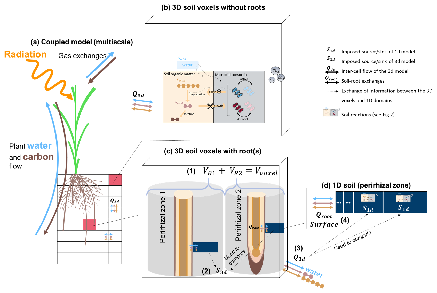
Figure 1 Representation of the multiscale coupling with (a) the whole multiscale model, (b) example of a 3D soil voxel without roots, (c) example of a 3D soil voxel with two roots, (d) example of a 1D model representing the whole perirhizal zone around a root segment. The 3D soil model (black grid) is made up of 3D voxels (transparent rectangles with black borders). The 1D model is represented using the dark blue line in the 3D voxels. It lies between a root segment and the end of the implicitly-represented perirhizal zone (grey hollow cylinder). (1) The sum of the volume of the perirhizal zones of the roots segments in a voxel is equal to the volume of the voxel. (2) The changes in content in the 1D models are used to define set sinks for the 3D voxels that contain at least one root. (3) The 3D flow entering or leaving a 3D voxel with roots is sent to the 1D models via sink terms in their sub-control volume. (4) The root releases and uptake are set as inner Neumann boundary conditions of the 1D soil models. The carbon-related reactions are computed in the voxels without roots and in the sub-control volumes of the 1D soils. More information on the reactions and the 1D models are given in Fig. 2.

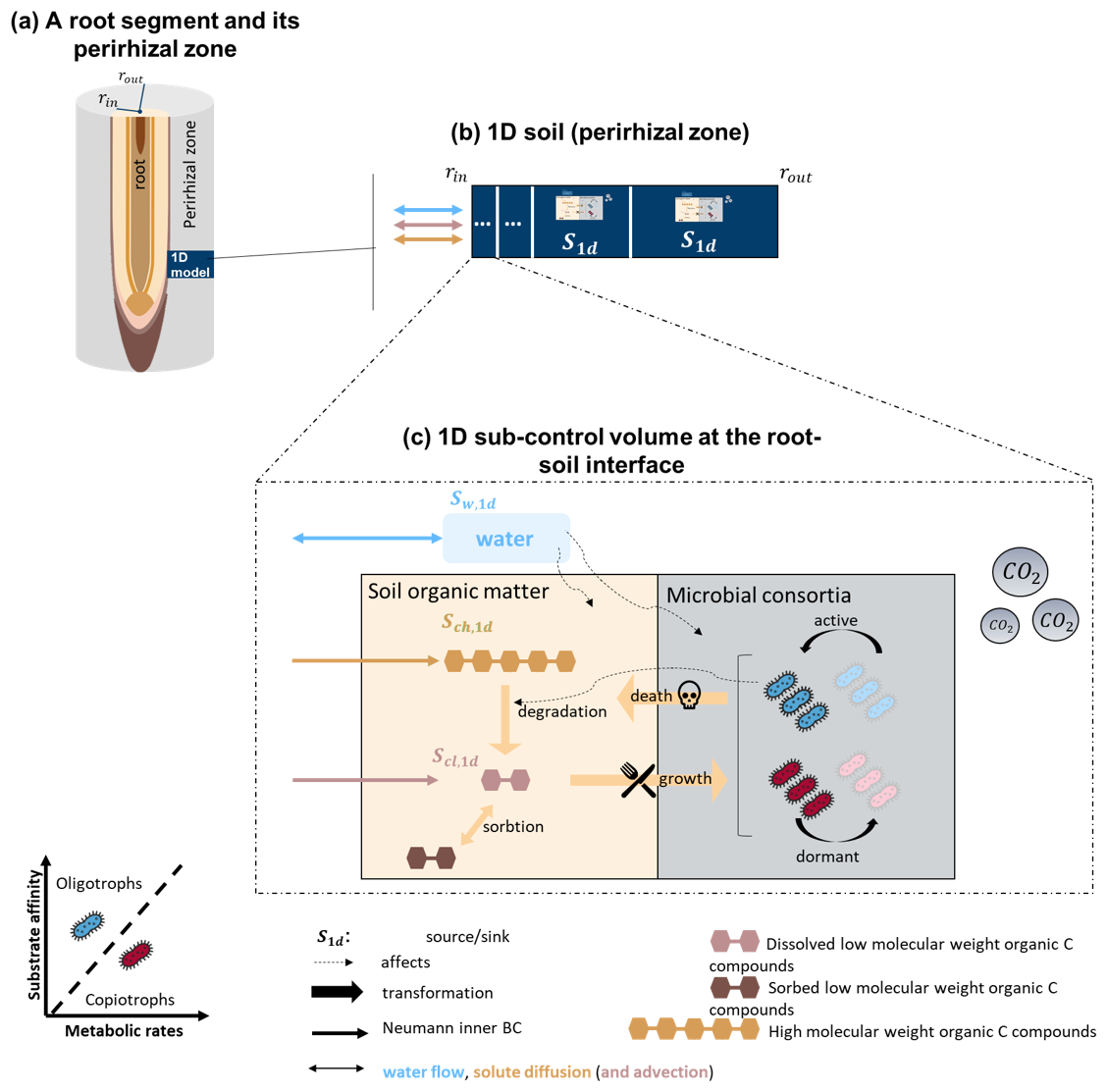
Figure 2 Representation of the updated 1D soil model (Sırcan et al., 2025) reimplemented within the multiscale framework (Mai et al., 2019; Koch et al., 2021). The model represents the soil domain around the root (perirhizal zone). Eight carbon pools are represented: carbon from organic compounds with a low molecular weight (dissolved and sorbed), organic compounds with a high molecular weight, active and dormant copiotrophs and oligotrophs, emitted microbial CO₂. Water flow and content are represented. Water affects the microbes (by impeding water stress) and the inert soil organic matter by lowering the dissolved carbon concentration. The graphic was adapted from Sırcan et al. (2025). The same reactions are also computed in 3D soil voxels that do not contain any roots (see Fig. 1).

Figure 3 gives a representation of the hard-coded direct interactions between the atmospheric conditions and the C and water pools represented in the plant and soil. For instance, high soil water content has a direct positive effect on the microbial development, as it stops the onset of water stress (see Eqs. D10, D29, D30). However, high soil water content also leads to a lower concentration of dissolved organic carbon. This lower dissolved carbon concentration was a negative effect on the microbial development by lowering the growth rate and making the microbes go into dormancy (see Eqs. D27, D28). It is the interactions between those processes that drive the water and C balances of the overall system. It is important to note that we represent the direct effects of temperature on plant processes but not on the microbial activity.

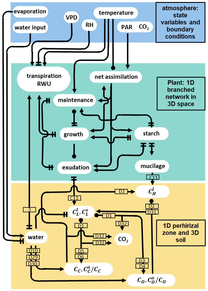
Figure 3 Graphical representation of the direct interactions represented between the different carbon and water pools plant model (green rectangle), soil models (yellow rectangle) and the atmospheric conditions given as input (blue rectangle). The lines ending with an arrow represent a positive effect, two perpendicular lines represent a negative effect, and a circle represents both a positive and negative effect (the net effect depends on the simulated conditions). The numbers in the rectangles give the indexes of the equations describing the corresponding process. The equations affecting the plant domain are defined in Giraud et al. (2023). The atmospheric conditions are represented by user-defined state variables and boundary conditions, e.g. vapour pressure deficit (VPD), relative humidity (RH), and incoming photosynthetically active radiations (PAR). Soil carbon pool data include the concentration of carbon from low molecular weight organic compounds in the soil and water phase (resp. $C_{\mathrm{L}}^{\mathrm{s}}$, $C_{\mathrm{L}}^{\mathrm{l}}$), high molecular weight organic compounds-C (C_H), total or active copiotrophs (resp. C_C, $C_{\mathrm{C}}^{\mathrm{a}}$) and oligotrophs (resp. C_O, $C_{\mathrm{O}}^{\mathrm{a}}$).

2.1.3 Temporal coupling

The modules of the plant and soil models are implemented sequentially. The order of the implementation is presented in Fig. 4. Each “outer” loop (encompassing all the modules) represents one time-step. Within each time step, two nested fixed-point iterations are implemented:

1. the “first fixed point iteration” contains the interactions between the (a) soil water flow and solute transport (for the 1D and 3D domains) and (b) plant water flow and stomatal regulation.

2. the “second (inner) fixed point iteration” links the steady state plant water flow and stomatal regulation. This iteration loop was presented in Giraud et al. (2023) and will not be detailed further here.

These two nested iteration loops allow for a higher computing speed. Indeed, the inner fixed point iteration for the stomatal opening can necessitate several hundred iterations before convergence (especially in the case of water-induced stomatal closing). While the FvCB-stomatal regulation module can compute these iterations quickly, the code section evaluating the water flow in the 3D- and 1D-domains is much slower. Moreover, in the first iterations of the FvCB-stomatal computation, strong over- or under-estimation of the transpiration may occur, especially in case of sharp changes in environmental conditions. Using these inputs directly for soil flow computation could lead to non-convergence errors. Processes in the C and water cycles can operate on different timescales (Gaudio et al., 2021). Specifically, the speed of plant growth and phloem transport tends to be slower than the plant and soil water flow. When running a simulation, it may consequently be necessary to use a smaller time step within the fixed-point iteration. Thus, we set up an adaptive operator splitting between the outer time step and the first fixed-point iteration, with an automatic adaptation of the fixed-point iteration time step. Moreover, we used an implicit time stepping within the fixed-point iteration when exchanging the results of the plant and soil domains, which means that the output of the previous loop is used as initial and boundary conditions for the next loop of the iteration. This implicit time stepping when coupling the three domains (plant, 3D soil, 1D soil) is more stable than the explicit alternative and allows us to use larger time steps, compared with earlier implementation of the multi-domain setup. Currently, the plant sucrose flow and growth are outside the iteration loop. Indeed, adding these modules to the fixed-point iteration would significantly slow the simulation. Also, for time steps <1 h, changes in plant shape and sucrose transport remain limited.

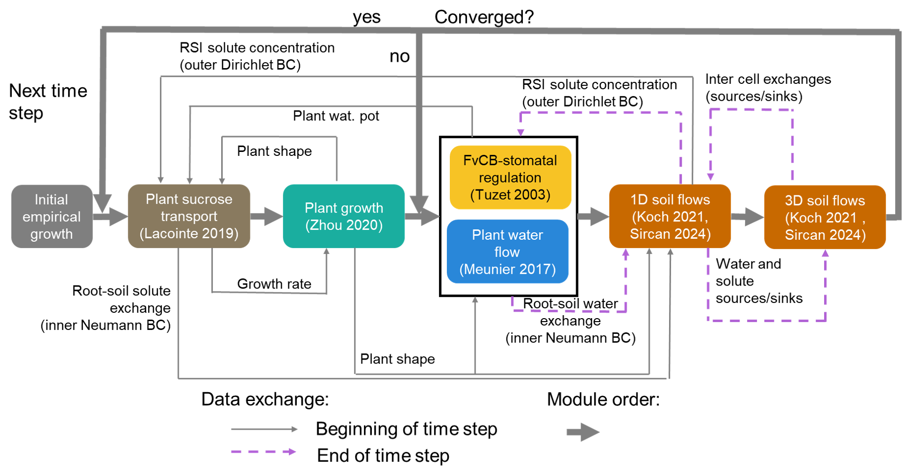
Figure 4 Representation of the time loop, as well as the implementation order and exchange of data between the modules. The loop including the soil flows (orange rectangles) corresponds to the outer iteration loop. The black rectangle outline containing the plant water flow (blue rectangle) and stomatal regulation (yellow rectangle) corresponds to the inner iteration loop. The plant sucrose transport and balance (brown rectangle) and growth (green rectangle) are not included in the iteration loop. Adapted from Giraud et al. (2023).

2.2 Governing Equations

These sections present the method used to simulate water and carbon turnover within the plant and the soil. Each section is divided between the plant-specific and soil-specific equations. For the soil part, the common equations for both the 3D and 1D soil models are presented, followed by equations specific to each domain. The soil volume (volume of the solid and pores) is written in cm³ scv (sub-control volume). The amounts of solutes and microbes are given in units of equivalent carbon (mol C). As the equations describing the microbial reactions remain similar to those set up by Sırcan et al. (2025), these ordinary differential equations are included in Appendix D.

2.2.1 Plant water flow

The plant water model is described in Giraud et al. (2023). Briefly, we compute the plant xylem water flow as:

$$\begin{array}{}\text{(1)}& {\displaystyle }-K_{\mathrm{ax},x}{\displaystyle \frac{{\partial }^{\mathrm{2}}{\mathit{\psi }}_{h,x}}{{\partial }^{\mathrm{2}}\mathit{\xi }}}=-p_{\text{seg}}\times q_{\text{w,plant-out}}\text{ for }\mathrm{\Omega }\backslash \partial \mathrm{\Omega },\text{(2)}& {\displaystyle \frac{\partial {\mathit{\psi }}_{h,x}}{\partial \mathit{\xi }}}=\mathrm{0}\text{ for }\partial \mathrm{\Omega }\text{ (all organ end-nodes)}\end{array}$$

K_ax,x (cm⁴ hPa⁻¹ d⁻¹) is the xylem intrinsic axial conductance and ξ (cm) is the local axial coordinate of the plant. p_seg (cm) is the perimeter of the plant exchange zone, Ω the domain considered (here the plant), and ∂Ω, the domain's boundary (here: the tip or end-node of each organ). We assume a no-flux boundary condition here as the plant-exterior water exchanges occur along the segments, therefore the equation given above is valid for the whole domain, except the boundaries $\mathrm{\Omega }\backslash \partial \mathrm{\Omega }$).

The net water sink is given by the lateral water flow (q_w,plant-out in cm d⁻¹), which corresponds to the xylem-soil (q_w,root-soil) or xylem-atmosphere (q_w,leaf-air) water exchange:

$$\begin{array}{}\text{(3)}& \begin{array}{rl}& q_{\text{w,plant-out}}=\\ & \left\{\begin{array}{rl}{q}_{\text{w,root-soil}}=min(k_{\mathrm{lat},x},k_{\mathrm{sri}})({\mathit{\psi }}_{h,x}-{\mathit{\psi }}_{\text{m,1DS}})& \text{, if root}\\ q_{\text{w,leaf-air}}=k_{\mathrm{lat},\min }({\mathit{\psi }}_{h,x}-{\mathit{\psi }}_{h,\mathrm{ox}})& \text{, if leaf blade}\end{array}\right.\end{array}\end{array}$$

With k_lat,x (cm hPa⁻¹ d⁻¹) the lateral hydraulic conductivity of the root cortex (for roots) or of the vascular bundle-sheath (for leaves) (Giraud et al., 2023, F.2.1). k_sri (cm hPa⁻¹ d⁻¹) is the equivalent lateral hydraulic conductivity and ψ_m,1DS (hPa) is the soil matric potential at the inner boundary of the corresponding 1D soil domain (root-soil interface). ψ_h,ox (hPa) is the water potential in the outer-xylem compartment, computed by the FvCB-stomatal regulation module. Note that, as changes in plant water storage are neglected, root water uptake equals transpiration at any given time step: ${\sum }_i^{\mathrm{segs}}{p}_i{q}_{\text{w,root-soil,}i}={\sum }_i^{\mathrm{nr}}{p}_i{q}_{\text{w,leaf-air},i}$, with p_i (cm) the perimeter of the segment i within the set segs.

k_sri is computed from the soil and plant data:

$$\begin{array}{}\text{(4)}& {\displaystyle }& {\displaystyle }{k}_{\mathrm{sri}}=\left\{\begin{array}{r}\frac{K_{\mathrm{sat}}{\mathit{\kappa }}_m\left(S_{\mathrm{sat}}\right)}{\mathrm{\Delta }{r}_{\text{root-1DS}}}\text{ if }{q}_{\text{w,root-soil}}\le \mathrm{0}\\ \frac{K_{\mathrm{sat}}}{\mathrm{\Delta }{r}_{\text{root-1DS}}}\text{ else }\end{array}\right.,\text{(5)}& {\displaystyle }& {\displaystyle }{K}_{\mathrm{sat}}={\displaystyle \frac{\mathit{\kappa }}{{\mathit{\mu }}_{\mathrm{w}}}}\end{array}$$

With K_sat (cm² hPa⁻¹ d⁻¹) the soil saturated hydraulic conductivity, μ_w (hPa d) the viscosity of the soil water solution, assumed equal to that of pure water at 20 °C. κ (cm²) is the intrinsic permeability of the soil and κ_m (–) the relative conductivity loss, dependent on the soil water saturation (S_sat, –). K_satκ_m(S_sat), the unsaturated hydraulic conductivity, is hereafter written as K for simplicity. Δr_root-1DS (cm) is the distance in radial coordinate between the root surface and the centre of the inner segment of the 1D soil domain. Net root water release (q_w,root-soil>0) is only limited by K_sat in the soil, while net root water uptake (q_w,root-soil<0) is also limited by κ_m.

2.2.2 Soil water flow

The variation in volumetric soil water content (θ in cm³ water (cm³ scv)⁻¹) is defined according to the Richards equations (Richards, 1931):

$$\begin{array}{}\text{(6)}& {\displaystyle \frac{\partial \mathit{\theta }}{\partial t}}=\mathrm{\nabla }\cdot \left(K\right(\mathrm{\nabla }{\mathit{\psi }}_{\mathrm{m},\mathrm{XDS}}-\mathrm{\nabla }{\mathit{\psi }}_{\mathrm{g},\mathrm{XDS}}\left)\right)+S_{\mathit{\theta }}\end{array}$$

With K (cm² hPa⁻¹ d⁻¹) the unsaturated hydraulic conductivity, ∇ψ_m,XDS and ∇ψ_g,XDS (hPa cm⁻¹) are the gradients of matric and gravitational water potentials in either the 3D (ψ_3DS) or 1D (ψ_1DS) soil domain, respectively.

S_θ (cm³ water cm⁻³ scv d⁻¹) is the net source of water in the domain. ∇ is the nabla operator, either for the 1D axisymmetric or for the 3D domain (Schey, 1973). We moreover have:

$$\begin{array}{}\text{(7)}& {\displaystyle }\mathit{\theta }=\mathit{\varphi }{S}_{\mathrm{sat}}\end{array}$$

with ϕ (cm³ pore (cm³ scv)⁻¹) the soil porosity (assumed constant). For simplicity, we assume that ϕ=θ_s, with θ_s (cm³ water (cm³ scv)⁻¹) the θ value at saturation. θ_r (cm³ water (cm³ scv)⁻¹) is the lowest possible θ value (residual water content). The hydraulic conductivity is defined using the pore size distribution model of Mualem (1976) and the water retention function is computed according to van Genuchten (1980):

$$\begin{array}{}\text{(8)}& {\displaystyle }& {\displaystyle }{S}_{\mathrm{sat}}={\left({\displaystyle \frac{\mathrm{1}}{\mathrm{1}+(\mathit{\alpha }{\mathit{\psi }}_{\mathrm{c},\mathrm{XDS}}{)}^n}}\right)}^{\mathrm{1}-\mathrm{1}/n}\text{(9)}& {\displaystyle }& {\displaystyle }{\mathit{\psi }}_{\mathrm{c},\mathrm{XDS}}={\mathit{\psi }}_{n,XDS}-{\mathit{\psi }}_{\mathrm{m},\mathrm{XDS}}\text{(10)}& {\displaystyle }& {\displaystyle }K={\mathit{\kappa }}_m\left(S_{\mathrm{sat}}\right)K_{\mathrm{sat}}\text{(11)}& {\displaystyle }& {\displaystyle }{\mathit{\kappa }}_m\left(S_{\mathrm{sat}}\right)=S_{\mathrm{sat}}^{l_{\mathrm{soil}}}\times {\left[\mathrm{1}-(\mathrm{1}-(S_{\mathrm{sat}}{)}^{n/(n-\mathrm{1})}{)}^{\mathrm{1}-\mathrm{1}/n}\right]}^{\mathrm{2}}\end{array}$$

ψ_n (hPa) is the reference pressure, set, for simplicity, at 1000 hPa, and ψ_c (hPa) is the capillary pressure. α (cm⁻¹) is related to the inverse of the air entry suction, n (–) is a shape parameter, l_soil (–) is the soil tortuosity. The implementations of Eq. (6) for the 3D soil and 1D soil are given respectively in Appendices B1 and B2.

2.2.3 Plant carbon transport

The plant sucrose model used for this study is based on the one presented by Giraud et al. (2023). The model was adapted to simulate mucilage release. The variation of sucrose-carbon concentration in the sieve tube ($C_{\mathrm{L}}^{\mathrm{st}}$ in mol C cm⁻³ st d⁻¹, with cm³ st the sieve tube volume) is computed from Eq. (12):

$$\begin{array}{}\text{(12)}& \begin{array}{rl}& {\displaystyle \frac{\partial C_{\mathrm{L}}^{\mathrm{st}}}{\partial t}}+{\displaystyle \frac{\partial }{\partial \mathit{\xi }}}\left(C_{\mathrm{L}}^{\mathrm{st}}\times K_{\mathrm{ax},\mathrm{st}}(R{T}_{\mathrm{seg}}{\displaystyle \frac{\partial C_{\mathrm{L}}^{\mathrm{st}}}{\partial \mathit{\xi }}}+{\displaystyle \frac{\partial {\mathit{\psi }}_{h,x}}{\partial \mathit{\xi }}}\right.\\ & \left.+{\displaystyle \frac{\partial {\mathit{\psi }}_{g,x}}{\partial \mathit{\xi }}})\right)-S_{\mathrm{exud},\mathrm{st}}-S_{\mathrm{starch},\mathrm{st}}-S_{\mathrm{other},\mathrm{st}}=\mathrm{0}\\ & \text{for }\mathrm{\Omega }\backslash \partial \mathrm{\Omega },t>t_{\mathrm{0}},\end{array}\end{array}$$

$$\begin{array}{}\text{(13)}& {\displaystyle }{K}_{\mathrm{ax},\mathrm{st}}\left(R{T}_{\mathrm{seg}}{\displaystyle \frac{\partial C_{\mathrm{L}}^{\mathrm{st}}}{\partial \mathit{\xi }}}+{\displaystyle \frac{\partial {\mathit{\psi }}_{h,x}}{\partial \mathit{\xi }}}+{\displaystyle \frac{\partial {\mathit{\psi }}_{g,x}}{\partial \mathit{\xi }}}\right)=\mathrm{0}\text{for }\partial \mathrm{\Omega }\text{(14)}& {\displaystyle }{C}_{\mathrm{L}}^{\mathrm{st}}=C_{\mathrm{L},\mathrm{0}}^{\mathrm{st}}\text{for }t=t_{\mathrm{0}},\end{array}$$

With ξ (cm) the local axial coordinate of the plant, R (hPa cm³ K⁻¹ mol⁻¹) the ideal gas constant, K_ax,st (cm⁴ hPa⁻¹ d⁻¹) the sieve tube axial intrinsic conductance, T_seg (K) the temperature of the plant segment. S_exud,st (mol cm⁻³ st d⁻¹) is the loss of $C_{\mathrm{L}}^{\mathrm{st}}$ by exudation of low molecular weight organic carbon compounds, S_starch (mol cm⁻³ st d⁻¹) is the loss or gain of $C_{\mathrm{L}}^{\mathrm{st}}$ by starch synthesis or degradation, S_other,st (mol cm⁻³ st d⁻¹) represents other net sinks of $C_{\mathrm{L}}^{\mathrm{st}}$–like gain by assimilation and inflow from the mesophyll compartment.

We assume that the exudation of low molecular weight organic carbon occurs via a passive diffusion (Rakshit et al., 2021; Ma et al., 2022), represented by a mass transfer approach:

$$\begin{array}{}\text{(15)}& {\displaystyle }& {\displaystyle }{S}_{\mathrm{exud},\mathrm{st}}=q_{\mathrm{exud}}{\displaystyle \frac{\mathrm{2}\mathit{\pi }{r}_{\mathrm{in}}L}{V_{\mathrm{st}}}}\text{(16)}& {\displaystyle }& {\displaystyle }{q}_{\mathrm{exud}}=k_{\mathrm{lat},\mathrm{st}}(C_{\mathrm{L}}^{\mathrm{st}}-C_{\mathrm{L}}^{\mathrm{l}})\end{array}$$

With k_lat,st (cm d⁻¹) is the lateral sieve tube conductivity for sucrose, V_st (cm³ st) is the sieve tube volume. We assume that exudation occurs mainly near the root tip (Rakshit et al., 2021; Badri and Vivanco, 2009; Neumann and Römheld, 2009). Therefore, $k_{\mathrm{lat},\mathrm{st}}>\mathrm{0}$ only for the last segment of growing roots. $C_{\mathrm{L}}^{\mathrm{l}}$ (mol C (cm³ water)⁻¹) corresponds to the concentration of dissolved low molecular weight organic carbon in the soil water at the root-soil interface. It is obtained from the inner segment of the 1D soil domain assigned to the root segment. We assume that the mucilage is made from starch (starch, in mol C cm⁻³) before being released via an active process (Rougier, 1981; Nguyen, 2009; Kutschera-Mitter et al., 1998). The production and release processes are represented in the following equations:

$$\begin{array}{}\text{(17)}& {\displaystyle }& {\displaystyle \frac{\partial \mathrm{starch}}{\partial t}}=S_{\mathrm{starch},\mathrm{st}}-S_{\mathrm{mucil},\mathrm{st}}\text{(18)}& {\displaystyle }& {\displaystyle }{S}_{\mathrm{starch},\mathrm{st}}=k_{\mathrm{targ},\mathrm{starch}}(C_{\mathrm{L}}^{\mathrm{st}}-C_{\mathrm{L},\mathrm{targ}}^{\mathrm{st}})\text{(19)}& {\displaystyle }& {\displaystyle }{S}_{\mathrm{mucil},\mathrm{st}}=q_{\mathrm{mucil}}{\displaystyle \frac{\mathrm{2}\mathit{\pi }{r}_{\mathrm{in}}{L}_i}{V_{\mathrm{st}}}}\text{(20)}& {\displaystyle }& {\displaystyle }{q}_{\mathrm{mucil}}=k_{\mathrm{mucil}}\mathrm{starch}\end{array}$$

With k_targ,starch (d⁻¹) and k_mucil (cm d⁻¹) parameters controlling respectively the synthesis and decay rate of starch and the release of mucilage. $C_{\mathrm{L},\mathrm{targ},\mathrm{st}}^{\mathrm{l}}$ defines the target $C_{\mathrm{L}}^{\mathrm{st}}$ and thus the threshold between starch synthesis and desynthesis. As in Hirschberg et al. (1998), the release of mucilage is represented via a simple first-order kinetic. We then obtain S_mucil (mol cm⁻³ st d⁻¹), the release rate of mucilage. k_mucil>0 only at the tip (in our model: the last segment) of growing roots. Both q_exud and q_mucil (mol cm⁻² d⁻¹) can then be used by the 1D soil domains (see Eqs. C13, C17).

2.2.4 Soil carbon transport

The changes in solute concentration are computed using the advection-diffusion-reaction equation – see Ahusborde et al. (2015) and Helmig (1997, Eq 3.100):

$$\begin{array}{}\text{(21)}& {\displaystyle }\begin{array}{rl}& {\displaystyle \frac{\partial \mathit{\theta }{C}_X^{\mathrm{l}}}{\partial t}}-\mathrm{\nabla }\cdot \left(C_X^{\mathrm{l}}{\mathit{u}}_X\right)-\mathrm{\nabla }\cdot \left(D_X\right(\mathit{\theta },\mathit{\varphi }\left)\mathrm{\nabla }{C}_X^{\mathrm{l}}\right)\\ & -S_X(-S_{\text{1DS–3DS},X})=\mathrm{0}\end{array}\text{(22)}& {\displaystyle }{S}_{\mathrm{ads},X}+S_{\mathrm{microbe},X}=S_X\end{array}$$

$C_X^{\mathrm{l}}$ (mol (cm³ water)⁻¹) is either the concentration of carbon from dissolved low molecular weight organic compounds ($C_{\mathrm{L}}^{\mathrm{l}}$) or high molecular weight organic compounds ($C_{\mathrm{H}}^{\mathrm{l}}$) in the soil liquid solution. S_X (mol C cm⁻³ scv d⁻¹) is the net source of $C_X^{\mathrm{l}}$, and it encompasses the adsorption of $C_X^{\mathrm{l}}$ (S_ads,X, mol C cm⁻³ scv d⁻¹, see Sect. 2.2.5) and the changes caused by microbial reactions (S_microbe,X, mol C cm⁻³ scv d⁻¹, see Appendix D and Eq. C1). S_1DS–3DS,X is an additional source term only used by the 1D soil models and presented in Eq. (C7). u_X is the advective flux.

D_X(θ,ϕ), the effective dispersion in the porous medium (caused by molecular diffusion and hydrodynamic dispersion), is obtained from Millington and Quirk (1961), as implemented by Koch et al. (2021):

$$\begin{array}{}\text{(23)}& {\displaystyle }{D}_X(\mathit{\theta },\mathit{\varphi })=D_{X\mathrm{w}}{\displaystyle \frac{{\mathit{\theta }}^{\frac{\mathrm{10}}{\mathrm{3}}}}{{\mathit{\varphi }}^{\mathrm{2}}}}\end{array}$$

With D_Xw (cm² d⁻¹) the diffusion coefficient of the carbon compound in water. Low molecular weight organic C compounds can be modelled as true solutes and are thus subject to convection. High molecular weight carbon compounds correspond to the plant mucilage releases, a gel-like substance when hydrated (Ma et al., 2022; Kutschera-Mitter et al., 1998). To simulate the rheology of mucilage slime, we adopt a simplified approach with a null advective flux (u_H) and a lower diffusion coefficient ($D_{\mathrm{H},\mathrm{w}}<D_{\mathrm{L},\mathrm{w}}$). For simplicity, the implementation of Eq. (21) for the 3D soil and 1D soil are given respectively in Appendices C1 and C2.

2.2.5 Adsorption

We describe in this section the adsorption of low molecular weight organic C compounds (C_L) from the liquid phase ($C_{\mathrm{L}}^{\mathrm{l}}$) onto the solid phase ($C_{\mathrm{L}}^{\mathrm{s}}$). As Sırcan et al. (2025), we describe the adsorption as linear. However, instead of equilibrium sorption, we used linear first-order kinetics. Not assuming instantaneous equilibrium allowed us to set lower time steps during the simulations. We further assume that only the low molecular weight organic substances can be sorbed. Adsorption was implemented according to Ahrens et al. (2020):

$$\begin{array}{}\text{(24)}& {\displaystyle }& {\displaystyle \frac{\partial C_{\mathrm{L}}^{\mathrm{s}}}{\partial t}}=k_{\mathrm{ads}}{C}_{\mathrm{L}}^{\mathrm{l}}(C_{\mathrm{L},\max }^{\mathrm{s}}-C_{\mathrm{L}}^{\mathrm{s}})-k_{\mathrm{des}}{C}_{\mathrm{L}}^{\mathrm{s}}\text{(25)}& {\displaystyle }& {\displaystyle }{C}_{\mathrm{L},\max }^{\mathrm{s}}=C_{\mathrm{L},\max }^{\mathrm{s}}={\mathit{\rho }}_{\mathrm{b}}{\displaystyle \frac{k_{\mathrm{clsmax}}{k}_{\mathrm{clay}+<\mathrm{20}\mathrm{\mu }\mathrm{m}\mathrm{silt}}}{M_{\mathrm{mass},\mathrm{C}}}}\end{array}$$

with k_ads (23265.14 cm³ scv mol⁻¹ C d⁻¹) and k_des (4.47 d⁻¹) the adsorption and desorption rates, defined according to the values given by Ahrens et al. (2020). $C_{\mathrm{L},\max }^{\mathrm{s}}$ (mol C cm³ scv) is the maximal concentration of adsorbed $C_{\mathrm{L}}^{\mathrm{s}}$, ρ_b (1.51 g mineral soil (cm³ scv)⁻¹) is the soil bulk density, M_mass,C (12.011 g C mol⁻¹ C) is the molar mass of carbon, $k_{\mathrm{clay}+<\mathrm{20}\mathrm{\mu }\mathrm{m}\mathrm{silt}}$ (0.45−, Wang et al., 2018) is the fraction of clay and silt smaller than 20 µm. k_cssmax (–) is an empirical factor defined according to the make-up of the clay minerals in the soil. According to Jiang et al. (2014), the Selhausen soil (used to calibrate the model) is dominated by illites, a 2:1 mineral. Consequently, k_cssmax=0.079 (Ahrens et al., 2020). This yields $C_{\mathrm{L},\max }^{\mathrm{s}}=\mathrm{4.5}\times {\mathrm{10}}^{-\mathrm{3}}$ mol C cm⁻³ scv. From the adsorption dynamic, we get the adsorption net sink for dissolved low molecular weight organic carbon: $S_{\mathrm{ads},\mathrm{L}}=-\frac{\partial C_{\mathrm{L}}^{\mathrm{s}}}{\partial t}$, used in Eq. (22). As high molecular weight organic carbon compounds represent the mucilage gel, no adsorption is represented: $S_{\mathrm{ads},\mathrm{H}}=\mathrm{0}$.

2.2.6 Plant growth and perirhizal zone

We simulate dynamic plants that grow according to input parameters (representing plants' genetically determined characteristics) and to their water and sucrose status (see Giraud et al., 2023). This leads to changes in root segment lengths and to the creation of new root segments. The method used to define the shape, water and solute content of new or growing 1D soil domains is presented below.

Currently, each root segment (and associated 1D soil domain) is allocated to the soil voxel containing its centre when the segment is first created, even if one or both segment extremities are out of the voxel. In order for the output to be realistic, it is therefore important for the maximum root segment size to be lower or near the length of a soil voxel. Moreover, for the current setup, root segments will remain in the same soil voxel even if the centre of an existing segment (because of segment elongation) moves to another voxel. We assume that these simplifications will have a limited influence on the results if the resolution is high enough. After simulating plant growth for the time step N, we obtain the new lengths (L, cm) and radius (r_in, cm) of the roots, which are, respectively, the lengths and inner boundary of the 1D soil domains. From these shape data, we recompute the distance to the outer radial boundary of each 1D domain (r_out, cm) according to the volume of the soil voxels (V_3DS,scv) and the number of 1D soil domains contained within (nr). For the 1D soil domain k in the voxel i:

$$\begin{array}{}\text{(26)}& {\displaystyle }{r}_{\mathrm{out},k}^N=\sqrt{{\displaystyle \frac{r_{\mathrm{in},k}^{\mathrm{2}}{L}_k^N}{{\sum }_j^{{\mathrm{nr}}_{i,N}}{r}_{\mathrm{in},j}^{\mathrm{2}}{L}_j^N}}{\displaystyle \frac{V_{\mathrm{3}\mathrm{DS}}}{\mathit{\pi }{L}_k^N}}+r_{\mathrm{in},k}^{\mathrm{2}}}\end{array}$$

Consequently, creation of new roots or changes in L and r_in of existing roots in a voxel can lead to changes in the perirhizal zone volume allocated to an individual 1D soil domain. From the soil point of view, a higher density of roots in the voxel leads to smaller perirhizal zones for each of the root segments contained in it. The description of the method used to update the amounts of water and carbon in the 1D soil models as they are created and change shape is presented in the Appendix E. In brief, the gradient of existing 1D domains with decreasing volume is preserved. We then compute the volume of newly freed soil for each voxel. From the amount of water and carbon lost by the 1D models, we obtain the mean water content and carbon concentration in the freed space. This volume (and corresponding water and solute contents) is distributed between the new and expanding 1D soil domains to respect the results of Eq. (26).

2.3 Model application: The effect of dry spells on soil carbon and microbial dynamics near a growing plant

The implementation setup for the coupled model follows that used in Giraud et al. (2023) (see Table A3). We simulated the growth of a C3 monocot under a control scenario (hereafter called baseline) and compared it with dry spells at two plant development stages. Both dry spells were represented by a period of one week without rainfall: 11 to 18 and 18 to 25 d after sowing, hereafter called earlyDry and lateDry. The periods of the dry spells were taken from Giraud et al. (2023). The start of the earlier spell was set late enough to assume that the seed no longer affected the plant's carbon balance. The end of the late spell was set early enough to finish before the end of the plant's vegetative growth, as the development of flowers, seeds and fruits is not yet implemented within CPlantBox. The virtual plants were obtained by running the plant model up to day 10 (after sowing) using a mean empirical growth rate (neither dependent on the carbon- nor water-flow) and without simulation of the water and carbon fluxes. From the 10th day onward, we simulated the carbon and water fluxes and the carbon- and water-limited growth, as well as the soil carbon dynamic. The plants all grew under the baseline conditions with a static soil (constant mean ${\mathit{\psi }}_{\mathrm{m},\mathrm{soil}}=-\mathrm{100}$ cm at hydraulic equilibrium), except during the dry spells: day of growth 11 to 18 for earlyDry, and 18 to 25 for lateDry. At the start of the dry spells, the mean soil water potential was lowered to −450 cm and warmer and drier atmospheric conditions were simulated (see Table 1. After the dry spells, the baseline environmental and static soil water conditions were used. We used a no-flux boundary condition for the 3D soil. Figure 5 summarises the timeline of the three scenarios.

Table 1 Environmental variables. Taken from Giraud et al. (2023).

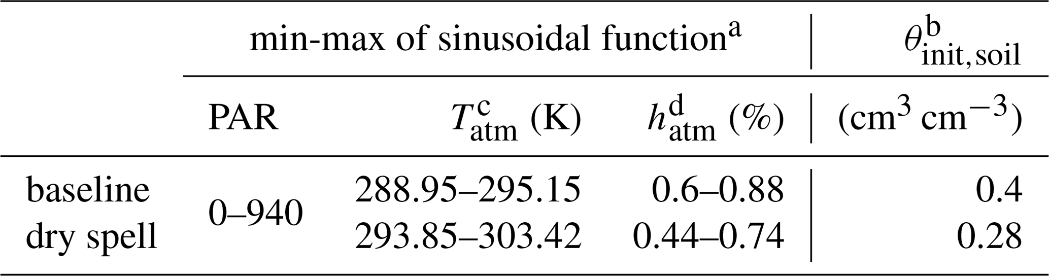
^a T_atm, PAR and h_atm go from their minimum to their maximum value via a sinusoidal function with a period of 1 d to represent the day-night cycle. All the atmospheric variables correspond to values 2 m aboveground. ^b θ_init,soil is the value of the constant soil water content of baseline; and it corresponds to the initial value of the dynamic soil water content for the dry spell periods. ^c T_atm is the air temperature. It affects only the plant processes and not the microbial activity. ^d relative air humidity. The baseline variables were used for all simulations before and after the dry spells

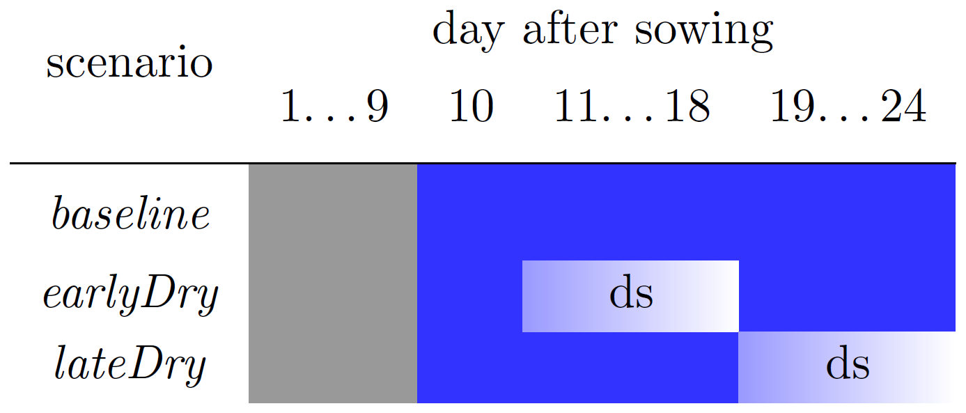
Figure 5 Timeline of the simulations. The grey (resp. blue) cells indicate the empirical (resp. semi-mechanistic) growth period and “ds” the implementation of the dynamic soil. The blue gradient during the dynamic soil simulation represents the decreasing soil water content. The sharp shift from dark to light (resp. light to dark) blue at the beginning (resp. end) of the dry spells represents the implementation of the dry spell (resp. baseline) atmospheric and initial (resp. constant) soil variables. Figure taken from Giraud et al. (2023).

For the plant model, the calibration of Giraud et al. (2023) was adapted to better follow our assumptions regarding the plant mucilage and carbon dynamic (e.g., preferential carbon usage for growth over exudation), and to address the divergences between the outputs of Giraud et al. (2023) and experimental observations (light dry spells caused carbon rather than water scarcity). Changes were also made to the lateral conductivity (k_lat,x, cm hPa⁻¹ d⁻¹) in the mature root zone: the constant value was computed according to Bramley et al. (2007, Fig. 4.15) and set to 1.5 % of k_lat,x within the immature root zone, see Appendix H for a more detailed description.

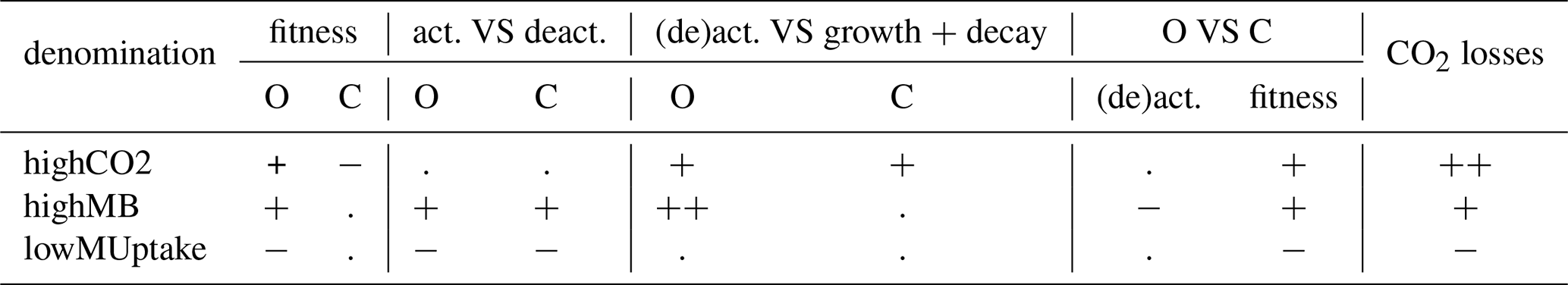
The selection of the kinetic parameter sets is given in Appendix I. Briefly, Sırcan et al. (2025) computed 1650 parameter sets respecting parameter and process constraints defined according to a literature review. Those sets were divided into three groups according to the resulting radial concentration profile of the low-weight dissolved organic molecules-C for the 1D soil domains. 33 sets were selected randomly from each group and a simulation was run for four days. We then selected three parameter sets giving diverging results. Table 2 presents the characteristics of the selected sets. The first set, thereafter called highCO2, led to a high CO₂ production in spite of a low microbial development. The second set, thereafter called highMB, led to the highest microbial development. The third set, thereafter called lowMUptake, led to the highest soil solute concentration (low microbial solute uptake).

Table 2 Qualitative summary of the characteristics of the three selected kinetic parameter sets (highCO2, highMB, lowMUptake). O: oligotrophs, C: copiotrophs, (de)act.: activation and deactivation, VS: compared against. The evaluation has the following order (representing the low-to-high gradient): $-<.<+<++$

2.4 Analysis of the outputs

The data were treated and visualised with Python3.10 (Python Software Foundation, 1995).

2.4.1 Scale definition for model evaluation

To take advantage of the multiscale setup, we evaluated the model outputs at four different scales: 3D scale, aggregated perirhizal scale, 1D scale. We define the 3D scale as the soil voxels (Fig. 1b) that contain at least one root at the end of the simulations in any of the scenarios. This soil space is therefore constant and equal for all simulations. We define the aggregated perirhizal volume as the 3D data of voxels containing at least one root at each time step, potentially different for each simulation. At the 1D scale, we evaluated the data for each segment of the 1D models (Fig. 1c) individually. Therefore, the 1D scale covers the same area as the aggregated perirhizal volume but represents a higher resolution: one data point for each sub-control volume of the 1D-models, against one data point for each sub-control volume of the selected 3D soil voxel. A graphical representation of the different scales is given in Fig. J1.

2.4.2 Vertical concentration profiles

To evaluate the vertical concentration profiles, we computed the total soil volume, water volume, and C content (for each C pool) for each depth at the aggregated perirhizal scale. This allowed us to determine the corresponding mean C concentration and water content around the root systems. Additionally, we present the minimum and maximum C concentrations (for each C pool) and water content values at each soil depth to capture the lateral variability.

2.4.3 Relative change of soil carbon distribution

To evaluate the change in plant-soil C turnover for the different weather scenarios and kinetic parameter sets, we categorised C into four pools: solutes (dissolved and sorbed low molecular weight organic C and high molecular weight organic C), microbes (including total oligotrophic and copiotrophic C), active microbes (including active oligotrophic and copiotrophic C), and emitted CO₂ (microbial respiration). We evaluated the C content at the 3D scale for each of these pools at each time step and normalised the values for earlyDry and lateDry under each kinetic parameter set according to the corresponding baseline scenario: $(C_{X,\mathrm{spell}}-C_{X,\mathrm{baseline}})/C_{X,\mathrm{baseline}}$, with X the name of the C pool.

2.4.4 Soil organic carbon hotspots

One important effect of plant C releases is the resulting changes in soil organic C (SOC). Using the study of Poeplau and Don (2023), we set three SOC thresholds defined according to the SOC $/$ SOC_expected ratio. These ratios correspond to the thresholds between soil quality classes: 0.65 (degraded to moderate soil quality), 0.83 (moderate to good soil quality), 1.16 (good to very good soil quality). These thresholds are used to distinguish hot spots. Since the studied scale in our study is much smaller than the one in the study of Poeplau and Don (2023), we only use their threshold value, but refrain from the qualitative interpretation. SOC_expected (mol C cm³ scv) is the average expected SOC according to the soil clay content. Following the method of Poeplau and Don (2023) and the Selhausen clay content data of Wang et al. (2018), we set SOC${}_{\mathrm{expected}}=\frac{{\mathit{\rho }}_{\mathrm{b}}}{\mathrm{1000}{M}_{\mathrm{C}}}(\mathrm{0.0288}{k}_{\mathrm{clay}}+\mathrm{13.674})=\mathrm{2.36}\times {\mathrm{10}}^{-\mathrm{3}}$ mol C cm³ scv, with k_clay the soil clay content in g kg⁻¹, ρ_b (g (cm³ scv)⁻¹) the soil bulk density, M_C (g C (mol C)⁻¹) the C molar mass. The $\mathrm{1}\times {\mathrm{10}}^{-\mathrm{3}}$ factor is used to go from g kg⁻¹ to g g⁻¹.

A first evaluation of the outputs showed that our simulated values were almost always in the lowest SOC class and significantly below the mean Selhausen SOC reported by Wang et al. (2018). For the hotspot analysis, we therefore added an SOC_slow class representing the very slow decomposing SOC, assumed to be constant over the study period. We set ${\mathrm{SOC}}_{\mathrm{slow}}={\mathrm{SOC}}_{\mathrm{theoric}}-{\mathrm{SOC}}_{\mathrm{simulated},\mathrm{init}}$, with SOC_{simulated,init} the total SOC explicitly simulated in our model (solute and microbial pools) at the beginning of the simulation, and SOC_theoric the value from Wang et al. (2018). We then set the variable $\mathrm{SOC}={\mathrm{SOC}}_{\mathrm{simulated}}+{\mathrm{SOC}}_{\mathrm{slow}}$, computed by the 1D soils. This is the value used to compare with the SOC thresholds given by Poeplau and Don (2023). We use a stacked area graph to represent the SOC hotspots, as soil above the higher thresholds is also above the lower thresholds. As presented by Landl et al. (2021a), we computed the volume-normalised hotspot volume. The relative hotspot volume was obtained by dividing the volume of each hotspot by the volume of all the 3D voxels that contained at least one root. Using a relative value allowed us to compare hotspot volume across root system architecture and age. The volume-normalised hotspot can be used as a metric for the efficiency of the rhizodeposition (Landl et al., 2021a).

2.4.5 Radial concentration profiles

Finally, for the 1D scale, we presented C concentration data for all segments of the 1D domains on one scatter plot per weather scenario and parameter set, giving, on the x-axis, the radial coordinate of the segment centers according to the root surface.

2.4.6 Complementary results

Some additional results, namely the complementary cumulative volume distributions, can give an overview of the status of the perirhizal zones of each simulation. However, as they do not affect the main conclusion of this work, these results and related analysis were moved to the Appendices K3, L and M.

3 Results

3.1 Three-dimensional simulation of microbial carbon dynamics in the soil-plant system

Figure 6 shows a typical simulation after 24.5 d of plant growth (midday) for a kinetic parameterisation that results in high microbial CO₂ production (highCO2) under the baseline scenario. The simulation highlights a concentration of dissolved low molecular weight organic C ($C_{\mathrm{L}}^{\mathrm{l}}$) and active copiotrophs ($C_{\mathrm{C}}^{\mathrm{a}}$) that increase with time in response to root exudation in the upper part of the root system, near its centre.

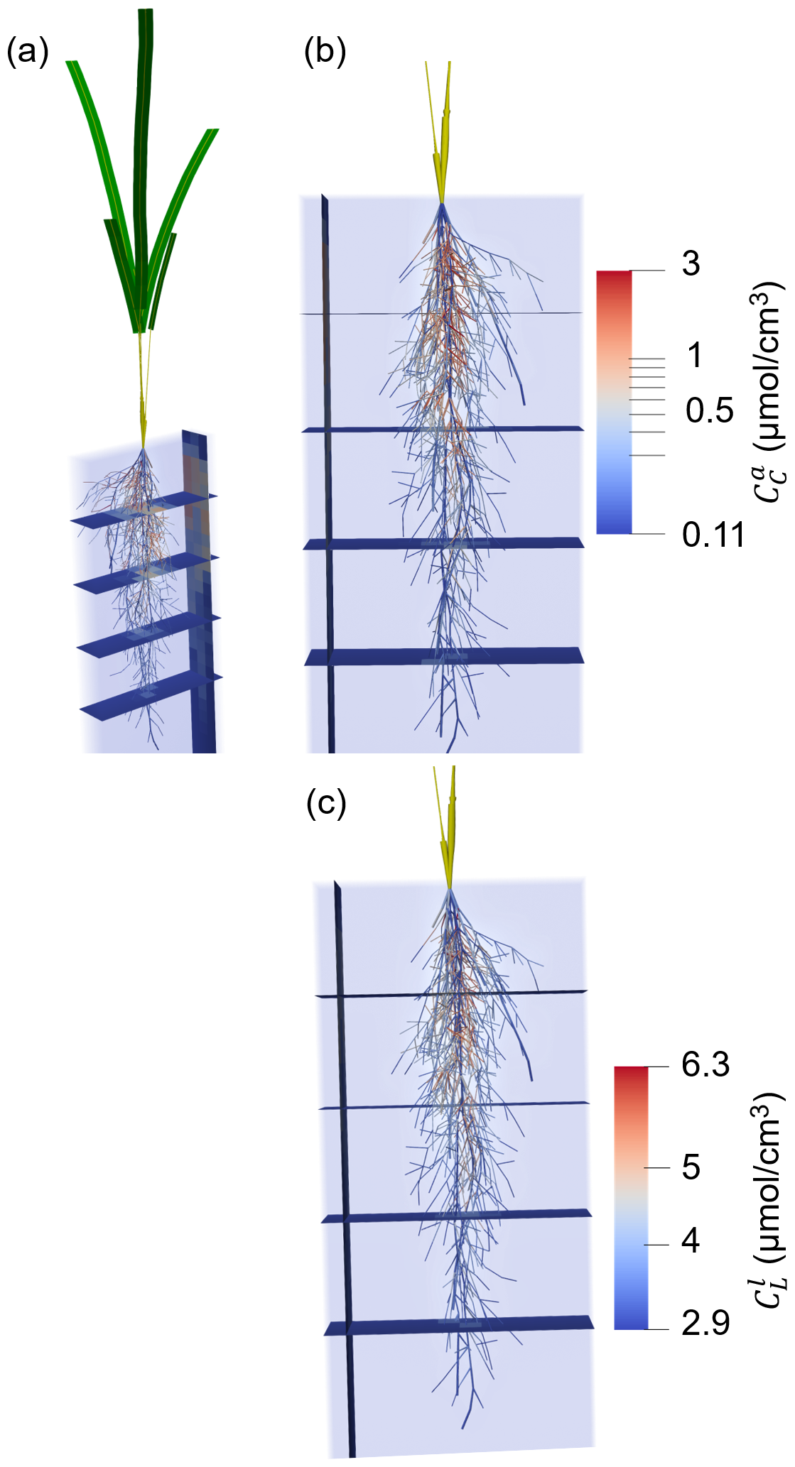
Figure 6 3D representation of the plant and soil domains for microbial kinetic parameterisation highCO2 under the baseline scenario at 24.5 d of growth, with (a) the whole plant, (b, c) zoom on the root system. (a), (b) present the concentration of active copiotrophic biomass C ($C_{\mathrm{C}}^{\mathrm{a}}$) and (c) that of dissolved low molecular weight organic C ($C_{\mathrm{L}}^{\mathrm{l}}$). The soil colours give the concentration in the aggregated perirhizal volume. The root colours give the concentration at the soil-root interface. Unified colours were given to the aboveground roots, shoot segments and leaf blades.

3.2 Plant processes

Figure 7A presents the plant xylem mean water potential (ψ_x, cm) for each kinetic parameterisation and weather scenario, while Fig. 7B shows the the cumulative amount of C used for growth (and growth respiration). As the focus on this study is the water and carbon dynamic within the perirhizal zone, the plant specific results are not included in the main body of the text. However, the outputs plant processes differ from those of Giraud et al. (2023). The plant results are therefore presented and discussed in Sect. K3. Figure 7C and D presents the cumulative amount of C used for (respectively) passive exudation and active mucilage release during the simulation. The plant water balance affected the exudation and mucilage release rate much more strongly than the kinetic parameterisation of the soil microbes. During the simulation, exudation occurred only under limited C use for growth in response to low plant water potential. Although the mucilage release was not always maintained at night (e.g., at the end of the earlyDry simulation), this process was less affected by the diurnal cycle than the exudation. This led to qualitative changes in the type of C released by the plant throughout the day. In comparison to baseline the early dry spell led to a lower total exudation at the end of the simulation: −32 %, −35 %, and −37 % for highCO2, highMB, and lowMUptake, respectively. Conversely, the late dry spell resulted in higher exudation compared to baseline: +29 % for highCO2 and highMB, +26 % for lowMUptake. Thus, the dry spells triggered both positive and negative effects on exudation. On the one hand, more C became available for exudation with decreasing plant growth. On the other hand, the lower xylem water potential led to a closing of the stomata, causing a lower assimilation rate per unit of leaf area.

Lower plant growth also led to lower leaf and total root surface area compared to baseline, which limited exudation. The effect of the simulated spells on total exudation was, therefore, dependent on the stage of plant growth at the start of the spell. After the end of the early dry spell (days 18–23), the daily plant exudation for earlyDry was higher than for baseline, partially reducing the exudation gap between the two. The total mucilage release under earlyDry at the end of the simulation was close to that under baseline: −11 %, −2 %, and +6 % for parameter sets highCO2, highMB, and lowMUptake, respectively. In contrast, mucilage release reached +139 % for highCO2 and highMB and +170 % for lowMUptake under lateDry. The highCO2 and highMB parameterisation, associated with high microbial C usage rates resulted in lower concentrations of dissolved low molecular weight organic C ($C_{\mathrm{L}}^{\mathrm{l}}$ mol C cm⁻³). This lower concentration of low-weight dissolved organic molecules-C increased passive exudation. The higher exudation was then compensated by the plant starch reserves (in the mesophyll and around the plant transport tissues) and did not affect the plant growth or maintenance. As the mucilage release rate is a function of the plant starch content, higher exudation induced lower mucilage release.

These differences in exudation and mucilage release appeared only after the onset of the dry spells. The release rates between the kinetic parameterisations for earlyDry became similar again from the third day after the end of the dry spell onward. The highest exudation rate per unit of root surface for a single segment across all simulations was obtained at 11 d 5 h with baseline and lateDry (0.153 mmol C cm⁻² d).

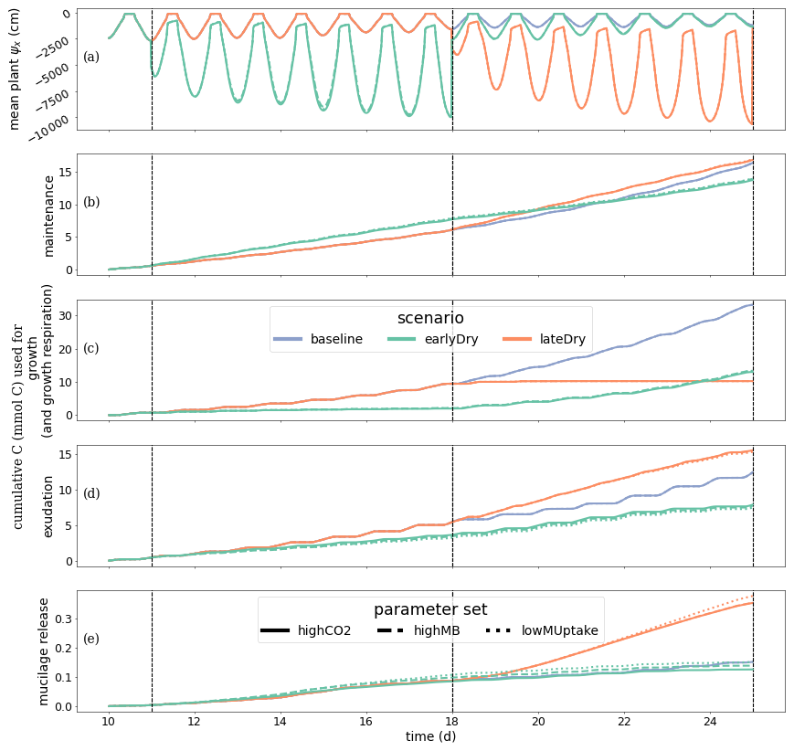
Figure 7 Dynamics of Plant water- and carbon-related metrics: (A) the mean plant xylem water potential (ψ), (B) cumulative carbon growth and growth respiration, (C) exudation, (D) mucilage release. Line colours indicate the weather scenarios: baseline (blue) against an early (green) and late (red) dry spell. Line types represent different kinetic parameter sets. The vertical dotted lines show the beginning and end of the early (day 11 to 18) and late (day 18 to 25) dry spells. Please note that the scales of the y-axis differ in each subplot.

3.3 Vertical concentration profiles

Figures 8 and 9 present the vertical concentration profiles of organic C, microbial pools and produced CO₂ from microbial respiration at the end of the simulation for the aggregated perirhizal scale. The root system structure affected the concentration profiles. The peaks of organic C between 0 and 13 cm of depth corresponded with the location of the highest root tip density (Figs. 8 and K1). A second peak of maximum C concentration was observed at the bottom of the profile close to the tips of primary roots. Moreover, the higher lateral dispersion of the roots in the upper soil layers led to a stronger lateral variability in the concentration profile (larger min-max ranges).

The kinetic parameterisation strongly influenced the C concentration profiles (Fig. 9). With highCO2, solute and microbial C concentrations were lowest: $\mathrm{3.5}\pm \mathrm{0.49}{C}_{\mathrm{L}}^{\mathrm{l}}$, $\mathrm{77.96}\pm \mathrm{9.25}{C}_{\mathrm{L}}^{\mathrm{s}}$, 595.72 ± 6.99 C_H, 10.17 ± 0.79 C_C, 9.31 ± 0.02 C_O, all in µmol cm⁻³. The highMB parameterisation also led to low solute concentrations but triggered increased microbial C due to higher microbial C consumption: $\mathrm{2.48}\pm \mathrm{0.20}{C}_{\mathrm{L}}^{\mathrm{l}}$, $\mathrm{55.96}\pm \mathrm{2.98}{C}_{\mathrm{L}}^{\mathrm{s}}$, 698.46 ± 7.76 C_H, 22.50 ± 8.44 C_C, 9.49 ± 0.04 C_O, all in µmol cm⁻³. With lowMUptake, solute concentrations were highest because of low microbial C uptake: $\mathrm{8.18}\pm \mathrm{3.67}{C}_{\mathrm{L}}^{\mathrm{l}}$, $\mathrm{174.06}\pm \mathrm{67.33}{C}_{\mathrm{L}}^{\mathrm{s}}$, 651.78 ± 8.24 C_H, 12.19 ± 4.23 C_C, 9.39 ± 0.08 C_O, all in µmol cm⁻³. These results are consistent with the observations obtained during the model conditioning (see Appendix I).

The weather scenarios had a less pronounced effect on the concentration profiles than the kinetic parameterisation. We obtained $\mathrm{4.51}\pm \mathrm{2.62}{C}_{\mathrm{L}}^{\mathrm{l}}$, $\mathrm{98.87}\pm \mathrm{54.34}{C}_{\mathrm{L}}^{\mathrm{s}}$, 645.90 ± 42.18 C_H, 14.26 ± 6.77 C_C, 9.41 ± 0.10 C_O under baseline, $\mathrm{4.37}\pm \mathrm{2.56}{C}_{\mathrm{L}}^{\mathrm{l}}$, $\mathrm{96.33}\pm \mathrm{53.12}{C}_{\mathrm{L}}^{\mathrm{s}}$, 647.53 ± 42.37 C_H, 14.16 ± 6.42 C_C, 9.38 ± 0.07 C_O under earlyDry, and $\mathrm{5.47}\pm \mathrm{4.68}{C}_{\mathrm{L}}^{\mathrm{l}}$, $\mathrm{116.66}\pm \mathrm{87.57}{C}_{\mathrm{L}}^{\mathrm{s}}$, 655.15 ± 43.45 C_H, 17.15 ± 9.87 C_C, 9.40 ± 0.08 C_O under lateDry, all in µmol cm⁻³. For each kinetic parameter set, earlyDry led to concentration profiles close to that of baseline, e.g., copiotrophs-C (in µmol cm⁻³): respectively 10.03 ± 0.69 and 9.98 ± 0.59 for highCO2, 20.64 ± 6.86 and 20.88 ± 6.86 for highMB, 11.74 ± 3.32 and 11.91 ± 4.75 for lowMUptake (Fig. 9). In particular, despite the lower total exudation, the concentration of low-weight dissolved organic molecules-C for earlyDry is close to that of the baseline due to the increased exudation rate during the second half of the simulation (Figs. 7, 8): respectively (in µmol cm⁻³): 3.36 ± 0.32 and 3.62 ± 0.63 for highCO2, 2.50 ± 0.14 and 2.54 ± 0.25 for highMB, 7.24 ± 2.59 and 7.36 ± 2.72 for lowMUptake. Under lateDry, we observed higher concentrations of high molecular weight organic compounds-C: $+\mathrm{1}\pm \mathrm{0}$ % compared with the baseline. This can be attributed to higher plant mucilage release for this scenario (Fig. 8). lateDry led to an increase in the mean concentration of activated oligotrophs-C compared with baseline: $+\mathrm{81}\pm \mathrm{64}$ % with highCO2, $+\mathrm{82}\pm \mathrm{74}$ % with highMB, $+\mathrm{251}\pm \mathrm{276}$ % with lowMUptake. However, the overall highest concentration values of activated oligotrophs-C and copiotrophs-C at the last time step were obtained with baseline (Fig. 9). The high amount of activated microbial biomass can partly be explained by the water content remaining at the high default value (−100 cm) during the whole simulation under baseline. C uptake by copiotrophs for highCO2 and highMB was higher (high copiotrophs-C, and microbially respired C as CO₂ but lower low-weight dissolved organic molecules-C concentration) under lateDry (Fig. 8) – respectively for highCO2 and highMB: $+\mathrm{6.4}\pm \mathrm{2.1}$ and $+\mathrm{30.0}\pm \mathrm{12.0}$ copiotrophs-C, $+\mathrm{85.3}\pm \mathrm{34.3}$ and $+\mathrm{58.1}\pm \mathrm{24.6}$ microbially respired C, $-\mathrm{6.5}\pm \mathrm{6.2}$ and $-\mathrm{6.3}\pm \mathrm{4.2}$ low-weight dissolved organic molecules-C compared with baseline. However, for lowMUptake, the higher C uptake by copiotrophs occurred under baseline, and under lateDry led to $+\mathrm{45.0}\pm \mathrm{17.7}$ low-weight dissolved organic molecules-C compared with baseline.

Due to the short simulation time, oligotrophs-C (Fig. 9) showed no significant growth at the aggregated perirhizal scale (<3 % of growth and <0.5 % of difference between the weather scenarios). Nevertheless, the dry spells weakly affected the proportion of active and dormant oligotrophs (Fig. 9): for lateDry compared with baseline, we observed $+\mathrm{19.0}\pm \mathrm{37.6}$ active oligotrophs-C with highCO2, $-\mathrm{42.9}\pm \mathrm{15.4}$ with highMB, $+\mathrm{28.6}\pm \mathrm{45.5}$ with lowMUptake.

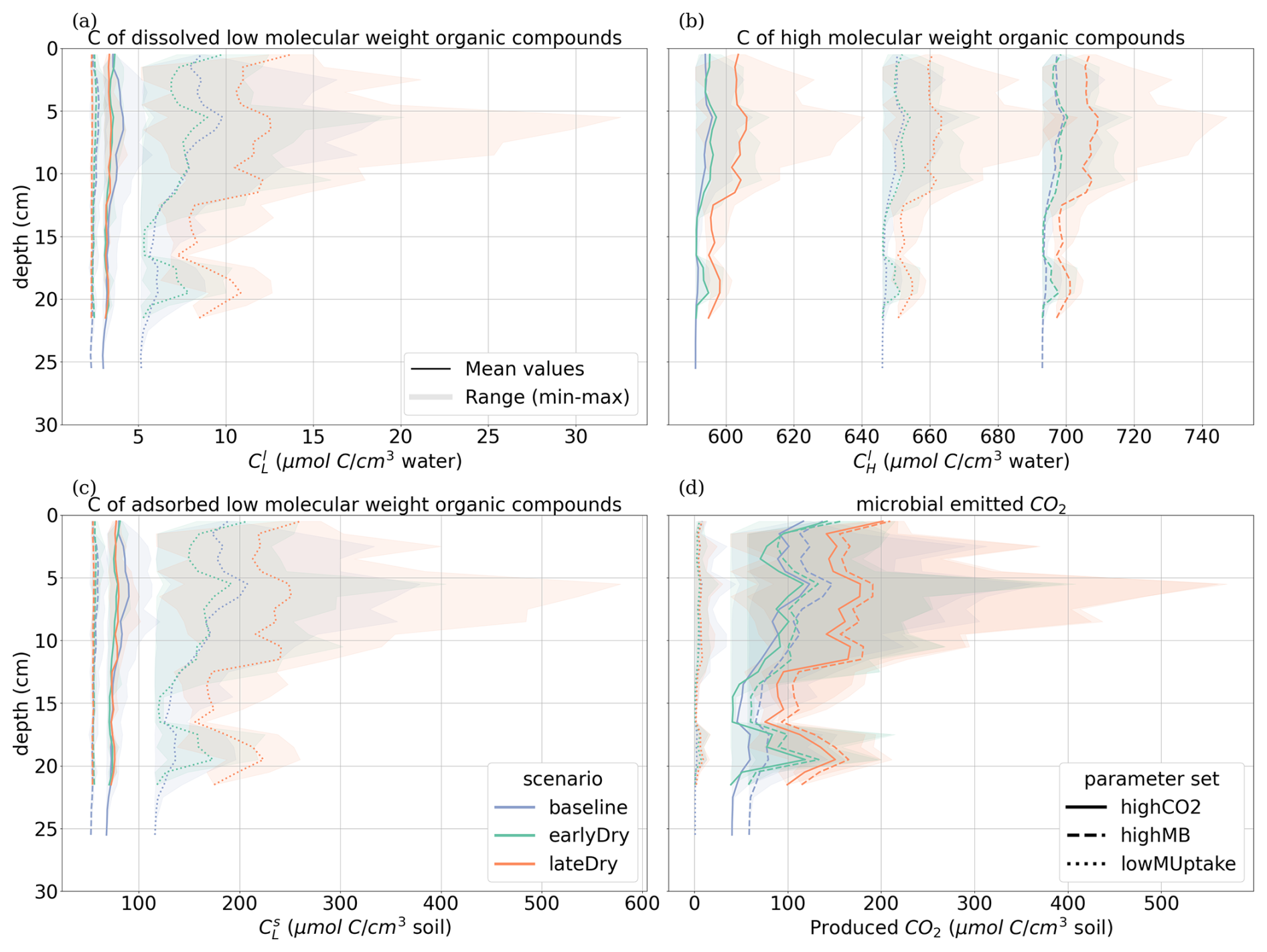
Figure 8 Mean concentrations of the soil carbon with depth within the aggregated perirhizal volume. (a) dissolved ($C_{\mathrm{L}}^{\mathrm{l}}$) and (c) sorbed ($C_{\mathrm{L}}^{\mathrm{s}}$) low-molecular-weight organic molecules-C, (b) high-molecular-weight organic molecules-C (C_H), (d) produced CO₂. Line colours indicate the weather scenarios: baseline (blue) against an early (green) and late (red) dry spell. Line types represent different kinetic parameter sets. The semi-transparent bands give the range between the minimum and maximum concentration in soil voxels with at least one root segment at each depth.

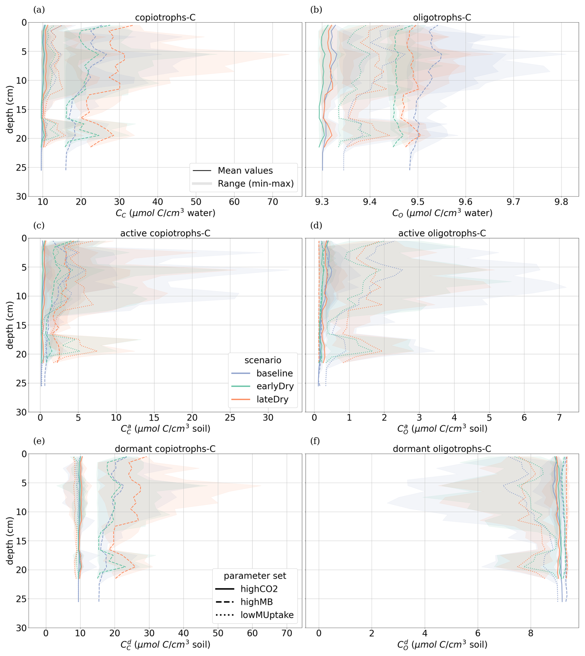
Figure 9 Mean concentrations of the soil carbon with depth within the aggregated perirhizal volume. (a, c, e) total (C_C), active ($C_{\mathrm{C}}^{\mathrm{a}}$) and dormant ($C_{\mathrm{C}}^{\mathrm{d}}$) copiotrophs, (b, d, f) total (C_O), active ($C_{\mathrm{O}}^{\mathrm{a}}$) and dormant ($C_{\mathrm{O}}^{\mathrm{d}}$) oligotrophs. Line colours indicate the weather scenarios: baseline (blue) against an early (green) and late (red) dry spell. Line types represent different kinetic parameter sets. The semi-transparent bands give the range between the minimum and maximum concentration in soil voxels with at least one root segment at each depth.

3.4 Carbon pool distribution

We wished to evaluate the changes in C turnover within the plant-soil system, according to the weather scenarios and for the different kinetic parameter sets. Consequently, Fig. 10 gives the relative changes of C content in different C pools, compared with the baseline scenarios. The relative increases of activated microbes-C and solutes-C (Fig. 10a and d) correspond to the night periods, when less C was exuded with baseline compared with the other scenarios. These periods also corresponded to higher soil matric potentials, diminishing the negative effects of the low soil θ on microbial activation during the dry spells. This relatively higher activated microbes-C pool was observed for the highCO2 and highMB parameter sets with lateDry (up to +50.0 % for highCO2 and +88.3 % for highMB), although the values were lower than for baseline at the last time step. The lateDry scenario led consequently to a redistribution of C in the microbial and emitted CO₂ pools. Therefore, in spite of the higher total exudation, the solutes-C pool is lower compared with the corresponding baseline scenarios (−2.7 % for highCO2 and −0.64 % for highMB). On the contrary, for lowMUptake, the lateDry scenario led to a higher accumulation of C within the solutes pools: +4.43 % (Fig. 10d). We can also note that, while we have converging relative solutes-C values between earlyDry and lateDry for highCO2 and highMB by the end of the simulations, the values for lowMUptake are diverging. For all earlyDry scenarios, less C entered the soil domain, leading to relatively lower values compared with baseline for all C pools (Fig. 10a–d) by the end of the simulations. We also found a small relative uptick of activated microbes-C for the highCO2 and highMB parameter sets after the spell (up to −2.3 % and +21.6 %, Fig. 10a), linked with the increased soil water content and plant exudation (Fig. 7). The same graphic is presented for the bulk soil in Appendix M1. Figure 10e shows the ratio of cumulative microbial-to-plant emitted CO₂ (see Figs. 7b, c and 10c). This ratio was strongly affected by the microbial parameterisation. At the end of the simulation, the ratio was 0.89 ± 0.2 for highCO2 and highMB, against 24.6 ± 1.8 for lowMUptake. Under lateDry, we observed an increase of the microbial-to-plant emitted CO₂ in spite of the higher plant maintenance respiration. This is higher maintenance respiration was, however, over-compensated by the lower growth respiration.

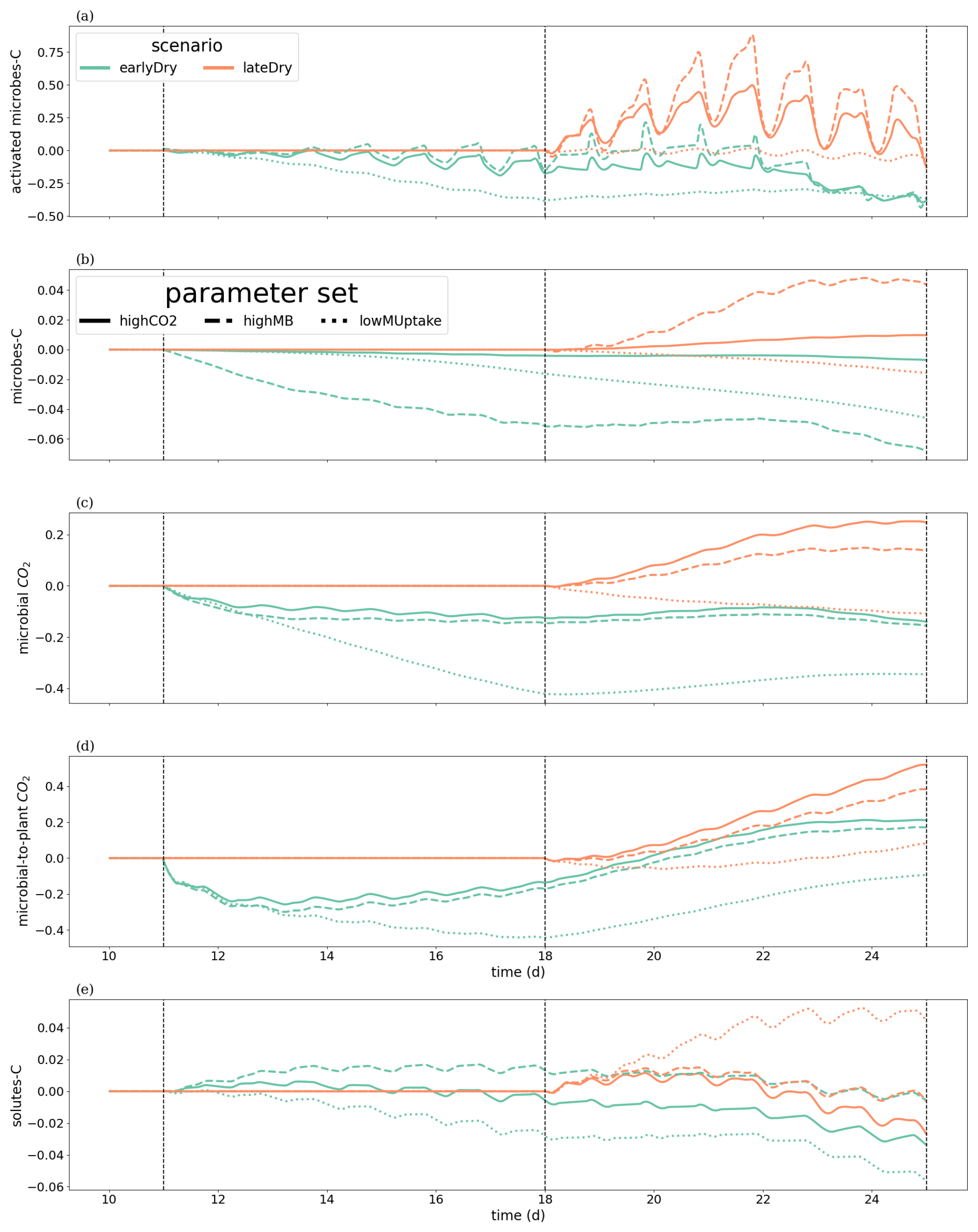
Figure 10 Relative change of carbon allocation in response to drought scenarios according to the kinetic parameters at the 3D scale. The panels present the difference of C between each drought treatment and the baseline in relation to the baseline C usage for (a) microbes-C, (b) activated microbes-C, (c) CO₂ emitted by microbes, (d) soil solutes-C, as well as (e) the difference in microbial-to-plant emitted CO₂. The line types represent the different kinetic parameterisation. The dotted lines show the beginning and end of the early (day 11 to 18) and late (day 18 to 25) dry spells. The line types represent the different kinetic parameterisation. Please note that the scales of the y-axis differ in each subplot.

3.5 SOC hotspots

To evaluate the root systems' exudation efficiency, Fig. 11 presents the relative volumes of the SOC hotspots (see definition in Sect. 2.4.4) in the aggregated perirhizal volume. We observed distinct characteristics over the whole simulation for each kinetic parameterisation. For highCO2, the absolute hotspot volume remained low and decreased with growth (after an initial increase during the dry spells). For highMB, the total absolute hotspot volume (SOC ≥0.65SOC_expected) peaked in the first half of the simulation before becoming stable under baseline. With this kinetic parameterisation, we observed the portion the relative hotspot volume within the highest class (SOC≥1.16SOC_expected): 8 %, 32 %, and 29 % of the hotspot volume belonged to the highest class under, respectively, baseline, earlyDry, and lateDry. Because of the low microbial activity, we observed the highest relative SOC hotspot volume for lowMUptake for all weather scenarios: $\mathrm{2.9}\times {\mathrm{10}}^{-\mathrm{2}}$, $\mathrm{2.8}\times {\mathrm{10}}^{-\mathrm{2}}$, and 0.11 under baseline, earlyDry, and lateDry.

Outside of the dry spell, diurnal cycling in the hotspot volume followed the plant C releases during the day and soil C mineralisation without replenishment at night. This dynamic is especially strong with highCO2 as the hotspot volume is (almost) back to 0 at the end of the day periods. The dry spells buffered the diurnal cycle for all scenarios as the exudation became more stable. Moreover, the biggest hotspot volume and intensity were obtained with the lateDry spell, following the higher exudation and mucilage release. earlyDry did not lead to a higher total hotspot volume (with SOC ≥ 0.65SOC_expected) for the highMB and lowMUptake parameterisation at day 25 of growth. However, a bigger portion of the SOC hotsposts belonged to the higher hotspot classes (≥ 0.83SOC_expected or ≥ 1.16SOC_expected).

For highCO2 and highMB, we observed an increase in hotspot volume during the first half of the dry spells, followed by a decrease during the second half. This can be partly explained by the decrease in daily plant C releases during the second half of the spell. The decreasing SOC hotspot volume in the second half of the spells was also due to the activation and growth of the microbial communities and C utilization after the first strong influx of plant C releases, followed by partial dormancy. Upon the next influx of C (the following day), the microbes reactivated and used the C more quickly. For lowMUptake, characterised by its lower microbial activity, we observed a continuous increase in hotspot volume throughout the spells.

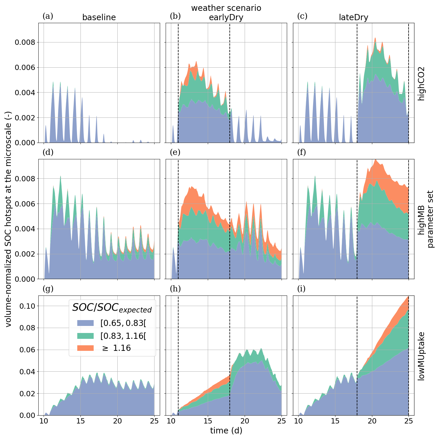
Figure 11 Relative SOC hotspot volume in the perirhizal zone according to time for the three $\mathrm{SOC}/{\mathrm{SOC}}_{\mathrm{expected}}$ classes. The classes' ranges were defined according to Poeplau and Don (2023). The dotted lines show the beginning and end of the early (day 11 to 18) and late (day 18 to 25) dry spells. The third row is on a scale different from the first and second rows.

3.6 Radial carbon concentration profiles

To analyse how plant-soil system responses to drought affect the carbon fluxes in the perirhizal zone, Fig. 12 shows the connection between the extent of the 1D soil domains and dissolved low-weight organic molecules concentrations $C_{\mathrm{L}}^{\mathrm{l}}$ at the end of the simulation. Just as for the aggregated perirhizal volume, the highest low-weight organic molecules-C concentrations were obtained under lateDry for lowMUptake (144.0 µmol cm⁻³) and under baseline for highCO2 (33.0 µmol cm⁻³) and highMB (24.0 µmol cm⁻³) (see Fig. M1). For lowMUptake, 1D domains with shorter outer radii (segment index eight, which is nearer to the root surface) had higher radial concentrations. These shorter outer radii were caused by several 1D domains sharing a single 3D scale voxel. The effect of high microbial C uptake with highMB is visible in Fig. 12d and e, where some concentration profiles show lower low-weight organic molecules concentration values closer to the root surface, where the concentration of copiotrophs-C is highest (see Appendix M). The radial concentration profiles of the low-weight organic molecules-C are strongly linked to the copiotrophs-C profiles, as presented in Appendix M.

The video “Video S2” (Giraud, 2026b) shows the low-weight dissolved organic molecules-C concentrations and the corresponding active-to-total copiotrophs-C ratios at each time step. We found a high microbial growth during the first pulse of added C followed by a transition to dormancy due to reduced C availability. Microbes remained mostly dormant until reactivated by the next C input pulse while also slowly dying. Reactivation of the microbes during the periods of high low-weight dissolved organic molecules-C concentrations led to a rapid consumption of the carbon in dissolved low-weight organic molecules near the root surface. As a result, $C_{\mathrm{L}}^{\mathrm{l}}$ became lower than it initially was once the C input pulse diminished–at night (e.g., day 24.69 of growth) and during the second half of the dry spells. We can also observe how, during the dry spells, low-weight dissolved organic molecules-C concentrations were higher than for the other two scenarios due to lower water content, favouring microbial C uptake.

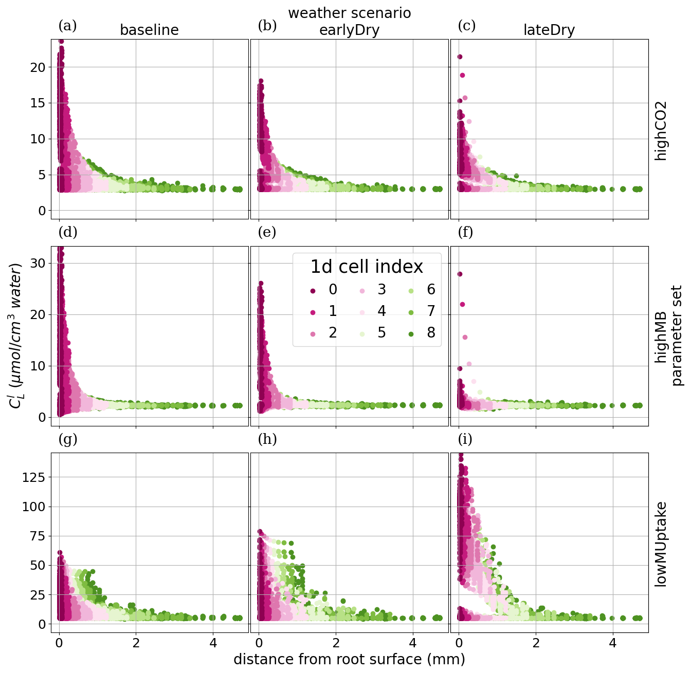
Figure 12 radial concentration profile of carbon from low molecular weight organic compounds at the end of the simulation for each plant perirhizal zone. r (mm) corresponds to the distance to the root surface. The colour gives the segment index of the 1D domain. Each column corresponds to a specific weather scenario and each row corresponds to a specific kinetic parameterisation.

4 Discussion

We developed a multiscale soil-rhizosphere-plant framework to evaluate the effects that a dry spell would have on the short-term soil carbon reactions, via shifts in plant processes. The results of our model were used to better understand diverging results observed for our selected calibration and scenarios. Our first hypothesis was that a dry spell would cause lower plant exudation. However, we observed that the drought could lead to both a decrease or an increase in cumulative exudation depending on the developmental stage of our simulated plant. Our second hypothesis was that the dry spell would lead to a lower microbial activity. For two of our three microbial calibrations, changes in total exudation led to the same trend in the microbial development and CO₂ emission when compared with the baseline scenario. For our last microbial parameter set lowMUptake, water stress caused by the dry spell was not compensated by higher plant exudation. Our last hypothesis was that drought could cause either an increase or a decrease in short-term carbon storage. For our simulations, we indeed observed both an increase and a decrease in the soil organic carbon.

In the first section of this discussion, we look in more detail at the simulated exudation. The main results of our study, regarding the simulated soil carbon dynamic and its changes under drought conditions, are discussed in Sect. 4.2.

4.1 Plant processes

In this implementation of the model, we simulated a simplified plant C dynamics compared with the one described in the literature, while still being able to reproduce qualitative plant dynamics. For a more detailed discussion of the plant related processes, see Sect. K3.

Like for our simulations, a decrease of rhizodeposits was experimentally observed at night (Kuzyakov and Cheng, 2004). This dynamic was particularly strong in our simulations, as we observed no exudation in the middle of the night outside of the dry spell periods. However, we could still recreate qualitative observations made in other studies. Indeed, plants regulate internal C concentrations and adjust C allocation for growth and maintenance under fluctuating environmental conditions by modulating starch storage (Tixier et al., 2023; Bazot et al., 2005) and C release rates (Prescott et al., 2020; Canarini et al., 2019). Also, the upper range of our exudation rates per unit of root surface was within the range found in the literature (Kravchenko et al., 2004; Trofymow et al., 1987; Personeni et al., 2007; Thorpe et al., 2011). The microbial C uptake affected the exudation rate by acting as a C sink (Canarini et al., 2019). We also observed a change in the type of organic C released by the plant (in our model, exudation-to-mucilage release ratio) under dry spell (Bazot et al., 2005; Hartmann et al., 2020). In spite of those changes, mucilage remained between 1 %–10 % of exudation, consistent with the observations of Nguyen (2009), and exudation represented between 3 %–40 % of assimilated C (Dilkes et al., 2004; Lynch and Whipps, 1990).

Regarding the plant water balance, the outputs of the model differ from those presented by Giraud et al. (2023), in part because of the change in our solver setup, in part because of the update of the plant parameters, as described in Sect. 2.3. After the update of the parameters, the starch reserves could be used more quickly by the plant when the assimilation rate became lower. This allowed for instance the plant to maintain its exudation rates at night. A further calibration of the plant carbon balance and its effect on the development of the surrounding microbes coudl be conducted thanks to study using positron emission tomography (Schultes et al., 2025).

4.2 Soil processes

4.2.1 Resolution of the multiscale setup

The output of the simulations showed diverging results according to the studied scales (larger scale in the 3D soil, smaller scale with the 1D models). These scale-dependent results underline the advantage of using a multi-scale simulation and having a higher precision at the root-soil interface, following the observations of Mai et al. (2019). Moreover, the model showed a strong horizontal and vertical variability in the concentrations, and different dynamics between the soil near or further away from the roots. For our setup, conducting a 3D evaluation remains relevant before, for instance, aggregating the results to a 2D or 1D sink term to be used by higher-scales models. As mentioned in the first implementation of the multiscale framework (Mai et al., 2019), the high resolution near the root soil interface (at the mm scale) raises the issue of including lower-scale processes, such as the influence of pore size on the water and C balance (Kuppe et al., 2022). As in the study of Landl et al. (2021a), the interactions between the 1D and 3D soil models also allowed us to represent the additive effect of perirhizal zone proximity, which led to higher solute concentration under specific kinetic parameterisation (lowMUptake) and favored C hotspot formation from plant releases. Landl et al. (2021a) also evaluated the influence of root traits on the soil's normalised hotspot volume. Our study complements those findings and shows that root and microbial traits have to be evaluated together, as high concentration of soil organic C can be reached for different exudation rates according to the traits of the microbial community.

4.2.2 Microbial starving-survival lifestyle

With the kinetic parameter sets highCO2 and highMB, we observed a diurnal dynamic of high microbial growth under higher exudation (daytime), leading to a high consumption of C for microbial growth and maintenance. This was followed by microbial dormancy (high dormant-to-total microbe ratio at nighttime). This dynamic has been observed in the literature and can be described as a “starving-survival lifestyle”, where microbes enter dormancy in a low-nutrient environment and quickly react to new inputs of resources (Hobbie and Hobbie, 2013). As highlighted by Hobbie and Hobbie (2013), this strategy represents the more common microbial strategy in natural systems.

Although our results depend strongly on modeling choices, this correspondence suggests that the outputs obtained with highCO2 and highMB may be more readily generalisable to real-world conditions.

Despite substantial differences in parameter values, the overall trends remained consistent between these two parameters (but not for the quantitative results). This stability may indicate the presence of conservative system behavior maintained by interactions among processes across a wide parameter space. A future study will include a comprehensive statistical analysis to more rigorously evaluate the influence of parameter variation on model outputs.

4.2.3 Microbial diversity

For highMB with lateDry, we found an especially high copiotroph growth and a high ratio of dormant-to-total oligotrophs. These diverging results between the two communities are indicative of a possible intra-microbial competition for this simulation. This follows over studies where plant exudation and root growth affected microbial composition (de la Fuente Cantó et al., 2020; Bonkowski et al., 2021). Although only two functional groups were represented, the higher development of the copiotrophs compared with the oligotrophs at the root-soil surface mimicked the lower microbial alpha-diversity observed experimentally in the rhizosphere (Kuzyakov and Razavi, 2019).

4.2.4 Priming effect

Kinetic parameter sets describing more active microbes (highCO2 and highMB) were also linked to a higher usage of soil solutes in case of higher exudation, when compared with the baseline scenarios. This higher usage rate led to a form of “rhizosphere priming effect” (Bonkowski et al., 2021; Kuzyakov and Cheng, 2004) where the root exudation can cause an increase in mineralisation of the pre-existing soil organic matter, leading ultimately to a relatively lower amount of C in the solute pool compared with the baseline. A more precise evaluation of a possible rhizosphere priming effect could be conducted with this setup, by dividing each C pool between the C originating from the plant additions and the C already present in the system at the beginning of the simulation. Moreover, in our simulation, the slower decomposing organic carbon pool was not explicitly represented (see Sect. 2.4.4), and we assumed that the pool would vary little over the short time scale represented. Including explicitly this carbon pool would allow for a more complete analysis of the carbon allocation and (increased) usage by the microbial community.

4.2.5 Microbial spatial distribution

Regarding the spatial resolution, we observed an effect of the root system structure and growth rate on the C concentration profile. The C concentration peaks observed for earlyDry and lateDry at deeper depth were due to lower root growth: The root tips remained in that area of soil over a longer period, leading to higher concentrations. Stronger plant growth under baseline resulted in perirhizal zones and rhizodeposition at lower depths such that the C accumulation at the root tips was much less pronounced compared to the dry spell scenarios. Moreover, for some of our scenarios, the high concentration of C pools at the outer boundary of our 1D model (lowMUptake) underlined the additive effect on the profile of the low-weight organic molecules-C due to proximity to the perirhizal zone, which can indicate an overlap of the rhizospheres. This proximity effect was less noticeable for highCO2 and highMB, where we observed concentration profiles less dependent on the extent of the 1D domain. Indeed, with those kinetic parameter sets, the microbial C uptake was highest and reacted fastest to high influxes of dissolved low molecular weight organic carbon. Therefore, the low-weight dissolved organic molecules-C concentration was closer to an asymptote at the outer boundaries of the 1D domain. These steeper gradients can cause the rhizosphere extent to be smaller, limiting the rhizosphere overlaps.

At the 1D scale, simulations also resulted in very high concentrations of copiotrophs near the root surface. Although high copiotrophic concentration near the root surface following exudation is expected (Bonkowski et al., 2021), representing microbial motility (Kuppe et al., 2022; Schnepf et al., 2022) would help smooth these concentration peaks, especially for older root segment with decreasing exudation and water uptake rates. Representing motility could also potentially lead to a better representation of the priming effect as the microbes (especially from mature roots) might diffuse and consume C in areas further away from the root-soil interface (Dupuy and Silk, 2016).

4.2.6 Sensitivity to water stress and carbon scarcity

The kinetic parameterisation strongly influenced the effects of the weather scenarios on soil C balance.

Our more active kinetic parameter sets (highCO2 and highMB), the microbial growth was limited by C resources. The higher plant C releases and lower soil water content lateDry had therefore a positive effect on the microbial community. On the contrary, for our non-C limited microbial communities (lowMUptake parameter set), the water stress of lateDry negatively affected the microbial growth. These opposite reactions influenced how the soil domain was impacted by the short dry spells (see below). Likewise, because of their lower potential maximum C uptake, oligotrophs profited more from wetter conditions.

The microbial dynamics will have an even stronger impact on the simulated water and C balance once soil-to-plant feedback mechanisms are implemented, such as nutrient uptake (de la Fuente Cantó et al., 2020) and organic C-dependent soil hydraulic parameters (Landl et al., 2021b; de la Fuente Cantó et al., 2020). Indeed, among other effects, mucilage increases the water holding capacity of the soil and can maintain hydraulic conductivity around the roots (Landl et al., 2021b; Carminati et al., 2016). This change of the hydraulic characteristics of the soil can affect the plant's capacity to withstand drought conditions.

4.2.7 Effects of dry spells

We could reproduce qualitatively processes measured by Deng et al. (2021) for the C balance under limited water resources. Indeed, we observed a decrease in root biomass during the dry spells, with, under some scenarios, an increased exudation. The lower root growth then led to lower plant respiration, while the higher concentration of dissolved organic C under the late dry spell (with highCO2 and highMB) led to a higher microbial respiration by the end of the simulation and a shift to a more microbial-dominated CO₂ emission. Contrary to Deng et al. (2021), we did not observe a decrease in total soil organic C. They linked this decrease to a lower soil C addition from plant residue, which is not represented in our model. Under lateDry, we could observe (limited) differences in concentration compared with the baseline seven days after the end of the dry spells, underlining the resilience of the simulated environment, especially for the soil zones nearer the roots.

4.2.8 Wetting-drying cycles

Our earlyDry and lateDry weather scenarios led to a short decrease in soil water content, creating a wetting-drying cycle. According to the meta-analysis of Borken and Matzner (2009), these wetting-drying cycles should lead, under specific environmental conditions and microbial communities, to lower microbial respiration during the spells, followed by a respiration pulse once the soil is rewetted (Birch effect). These pulses may or may not compensate for the earlier CO₂ emission decrease (Borken and Matzner, 2009). In our simulation, the early dry spell always led to a decrease in overall emitted microbial CO₂ at the 3D scale when compared with the baseline scenarios. We then observed in the week following the end of the spell a slight uptick in emitted CO₂ compared with the baseline, which did not compensate the lower earlier emissions. For the later dry spells with highCO2 and highMB parameterisation, the emission pulses occurred during the spells. Indeed, while the drying led to a lower portion of microbes being dormant, the soil water content often remained too high to cause high microbial death or deactivation, especially for soil zones further away from the roots (3D scale). The lower water stress was, therefore, partly compensated by the higher concentrations of low-weight dissolved organic molecules-C. We did not simulate an increase of plant and microbial necromass to be used by the soil microbes at the end of the spell (increasing thus the respiration once the soil is rewetted). Another explanation for the divergence is that we do not represent the easier access to “previously protected organic matter” caused by sudden soil rewetting. Moreover, we represented short dry spells (seven days) while longer spells (two weeks) may be necessary to see stronger effects on the microbial community (Borken and Matzner, 2009). The higher C mineralisation during the drying phase of the later dry spell could also be linked to the method used to represent microbial sensitivity to water stress. Indeed, for simplicity, we did not represent the direct effect of soil water content on the potential microbial death (k_max). Moreover, we used the same value to calibrate the sensitivity of copiotrophs and oligotrophs to water stress, although oligotrophs could be assumed to be more resistant to low soil water content. Finally, the water scarcity parameters could be recalibrated using experimental data.

4.2.9 Bottlenecks and future development

In theory, two non-microbial organic carbon pools can be used to represent the soil organic carbon (Sırcan et al., 2025; Kuppe et al., 2022). However, for this model setup, a third inert carbon pool was needed to accurately represent the C dynamic of slow decomposing organic matter. The reason for this limitation was twofold. First of all, to represent the movement of mucilage, our high-molecular weight organic C undergoes diffusion. Therefore, we only represent labile organic carbon. Moreover, our soil organic carbon concentration results (even in the perirhizal zone) were below the organic C concentration observed in Selhausen (Wang et al., 2018) and by Poeplau and Don (2023) for healthy bulk soil. This discrepancy was caused by our calibration. In their work Sırcan et al. (2025) conducted a review of acceptable ranges for each of their output variables. However the objective of their work was not to conduct an extensive review of the literature for each variable, and their maximum organic C concentration values were obtained from two studies: one conducted in Karnal (India) in a Typic Natrustalf soil with 34 % sand, 46.1 % silt and 19.9 % clay and the other in the Loess Plateau of the Gansu province (China) for a sandy-loam soil 1297 m above sea level. These two soils differed from the soil at our study site in Germany: a Haplic Luvisol in a temperate maritime climate zone (13.8 % sand, 68.4 % silt and 17.8 % clay). Conducting a more precise calibration for a specific experimental setup and introducing a non-labile carbon pool would allow the model to better represent the soil carbon dynamic. The implicitly represented slow decomposing soil organic carbon was assumed to be inert over the duration of the study, as our simulation time was of two weeks. However, not representing this third pool limits the generalisation that can be made of our results. For instance, the Birch effect discussed below is also caused by the destabilisation of this slow decomposing carbon pool after re-wetting of the soil (Borken and Matzner, 2009). This added pool also shifted the fractions of soil belonging to the different hotspot categories. For this reason, the thresholds of Poeplau and Don (2023) were presented as example categories to compare the scenario and evaluate changes over time rather than absolute value indicative of soil health.

Our simulation of the microbial dynamics and competition could also be improved by accounting for other stresses than C and water scarcity, such as nitrogen, phosphorus (Drake et al., 2013; Brown et al., 2022), or oxygen (Wiesenbauer et al., 2024) scarcity. Likewise, the diurnal aspect of microbial activity would also be better represented by accounting for soil temperature (Kuzyakov and Cheng, 2004).

5 Conclusions

In this paper, we presented the equations and implementation of a coupled model representing carbon and water flow in the soil-rhizosphere-plant continuum, influenced by atmospheric conditions through plant transpiration and photosynthesis. This framework accounts for the effects of water content variation on carbon flow and microbial activity. The multiscale implementation enables precise evaluation of fluxes and reactions at the soil-plant interface and can capture feedback across domains and scales. Despite the simplified representation of plant and microbial processes and limited calibration, the model reproduces trends reported in the literature, such as the “starving-survival” lifestyle of some microbial communities. We found that the effect of water scarcity on soil carbon turnover is an emergent property arising from 1D scale feedbacks between plants, microbes, and local environmental conditions. The varied impacts of water stress highlight the strong influence of local soil and plant characteristics in determining whether carbon or water limitation dominates turnover. By representing multiple sources of plant and microbial stress, the model provides a mechanistic explanation for variability in plant and soil carbon allocation under combined stresses. The model yields a wide range of variables across the soil-rhizosphere-plant continuum, such as short-term plant and soil carbon balance and exchanges. These outputs can be used to assess the performance of plant phenotypes and management measures under dynamic conditions using metrics like water and carbon uptake and use efficiency. By computing the resulting soil and plant conditions and identifying the key processes driving ecosystem responses, this model can both provide parameters for larger-scale models and inform the design of simplified models that focus on the most influential processes. Moreover, this work lays the foundation for a more comprehensive model of the plant-soil interaction cycle, including nutrient exchanges, which are essential to accurately represent the feedback of soil on plant processes. Finally, this model is particularly well suited to reproduce the experimental observations of isotopic carbon allocation in the plant and soil.

Appendix A: List of the parameters and variables

Table A1 Represented carbon pools.

(Moyano et al., 2013)(Wang et al., 2021)(Wang et al., 2021)(Moyano et al., 2013)(Moyano et al., 2013)(Wang et al., 2021)

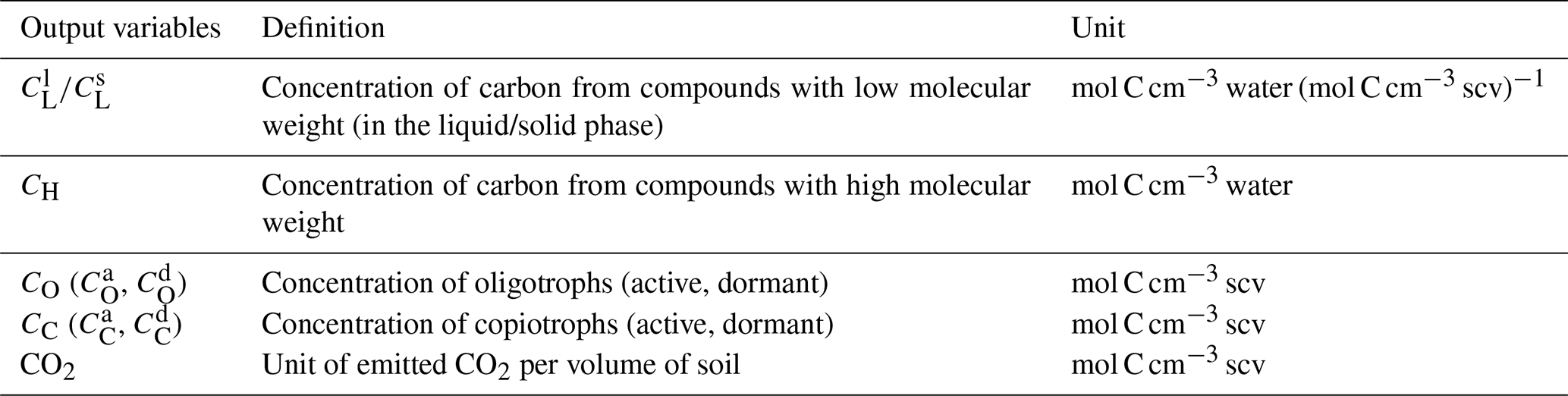
Table A2 Input parameters for the soil model. When the source is not given, the parameter values are taken from the sets defined by Sırcan et al. (2025) and selected in Sect. I. HMW: high molecular weight organic carbon compound.

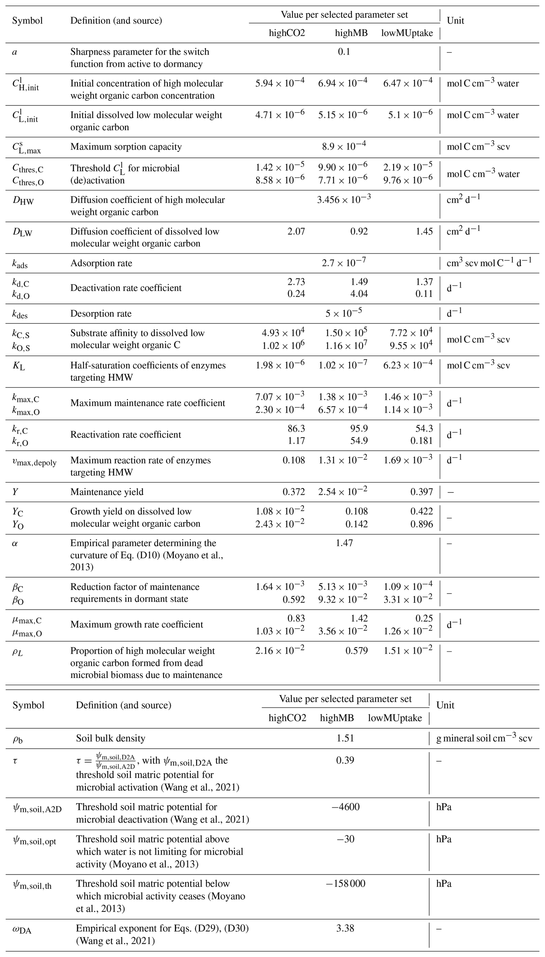
Table A3 Soil Van-Genuchten parameters. Taken from Giraud et al. (2023).

Appendix B: Soil water flow

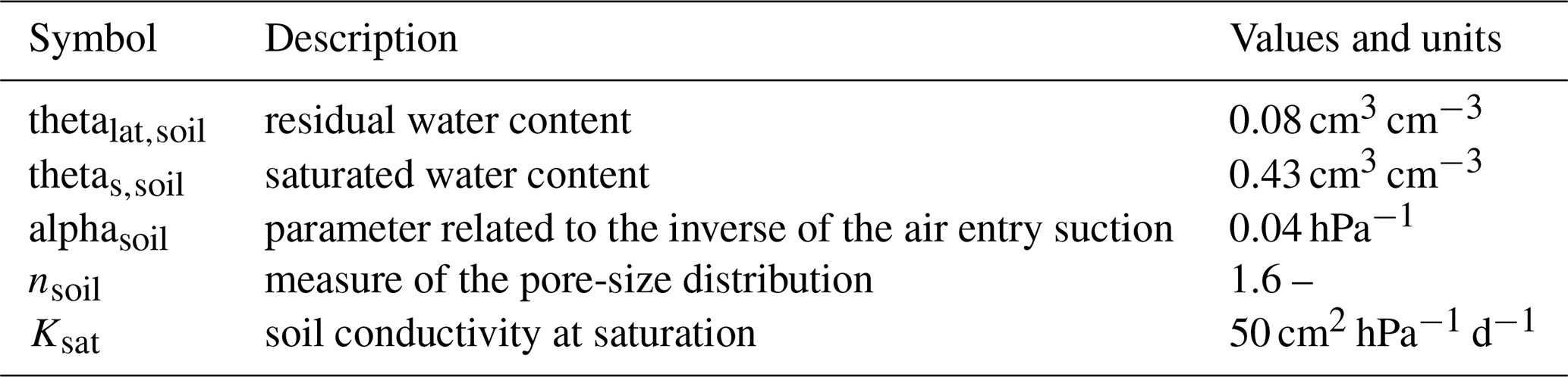
In the sections below, we present the implementation of the equations given in Sect. 2.2.2 to the 1D axisymmetric and 3D soil domains.

B1 3D soil model

For the 3D soil model, the sink term of Eq. (6) S_θ = S_{w, root-3DS} (cm³ water cm⁻³ scv d⁻¹), the water uptake or release by the roots:

$$\begin{array}{}\text{(B1)}& {\displaystyle }& {\displaystyle }{S}_{\text{w, root-3DS, init}}={\displaystyle \frac{\mathrm{1}}{V_{\text{3DS,scv}}}}\sum _{i=\mathrm{1}}^{\mathrm{nr}}{\displaystyle \frac{\partial {\mathit{\theta }}_i{V}_{\mathrm{1}\mathrm{DS},\mathrm{scv},i}}{\partial t}}\text{(B2)}& {\displaystyle }& {\displaystyle }{S}_{\mathrm{w},\mathrm{root}-\mathrm{3}\mathrm{DS}}=\mathbf{Lim}\left(S_{\mathrm{w},\mathrm{root}-\mathrm{3}\mathrm{DS},\mathrm{init}}\right)\end{array}$$

where nr (–) is the number of root segments in the soil control space of volume V_3DS,scv (cm³ scv), the i subscript is the identification of the ith root, $V_{\mathrm{1}\mathrm{DS},\mathrm{scv},i}$ (cm³ scv) is the volume of the perirhizal zone i and θ_i its water content. Instead of using q_w,root-soil (see Eq. 3) like Mai et al. (2019), in this study S_{w, root-3DS} is obtained from $\frac{\partial {\mathit{\theta }}_i{V}_{\mathrm{1}\mathrm{DS},\mathrm{scv},i}}{\partial t}$. This helps avoid computation errors when simulating the 3D-soil flows and diminishes the divergence between the 3D- and 1D-models. Indeed, the plant-prescribed q_w,root-soil was already potentially limited during the computation of $\frac{\partial {\mathit{\theta }}_i{V}_{\mathrm{1}\mathrm{DS},\mathrm{scv},i}}{\partial t}$ according to ψ_x,crit (see Eq. B12). We then set a second limitation on the net sink (resp. source) using the maximum potentially available water (resp. space) in the voxel–equal to the water (resp. space) volume at the beginning of the time step and to the maximum amount of water that could be gained (resp. lost) according to the inter-voxel flow at the last time step. The driving equation for the water flow is defined thus at the 3D scale (Mai et al., 2019; Koch et al., 2021):

$$\begin{array}{}\text{(B3)}& {\displaystyle }\begin{array}{rl}& {\displaystyle \frac{\partial \mathit{\theta }}{\partial t}}=K_{\mathrm{sat}}\mathrm{\nabla }\cdot \left({\mathit{\kappa }}_m(\mathrm{\nabla }{\mathit{\psi }}_{\text{m,3DS}}-\mathrm{\nabla }{\mathit{\psi }}_{\text{g,3DS}})\right)\\ & +S_{\text{w, root-3DS}}\text{ for }\mathrm{\Omega }\backslash \partial \mathrm{\Omega },t>t_{\mathrm{0}}\end{array}\text{(B4)}& {\displaystyle }{S}_{\text{w, root-3DS}}=S_{\text{w, root-3DS,0}}\text{at}t=t_{\mathrm{0}}\end{array}$$

A boundary condition completes the model and can represent, for instance, the net gain or loss of water resulting from rainfall and soil evaporation.

B2 1D axisymmetric soil models

Because of the small radii of the 1D domains, we assume that the gravitational gradient along the radial coordinate is negligible compared with the matric potential gradient: $\mathrm{abs}\left(\frac{\partial {\mathit{\psi }}_{\mathrm{g},\mathrm{1}\mathrm{DS}}}{\partial r}\right)\ll \mathrm{abs}\left(\frac{\partial {\mathit{\psi }}_{\text{m,1DS}}}{\partial r}\right)$. We thus get (Debnath, 2005, Eq. 1.10.4):

$$\begin{array}{}\text{(B5)}& {\displaystyle \frac{\partial \mathit{\theta }}{\partial t}}={\displaystyle \frac{\mathrm{1}}{r}}{\displaystyle \frac{\partial }{\partial r}}\left(r{K}_{\mathrm{sat}}{\mathit{\kappa }}_m{\displaystyle \frac{\partial {\mathit{\psi }}_{\text{m,1DS}}}{\partial r}}\right)+{\displaystyle \frac{\mathrm{1}}{r}}{S}_{\text{w, 3DS-1DS}}\end{array}$$

with r (cm) the radial coordinate along the axisymmetric domain, where r=0 corresponds to the center of root segment associated with the 1D soil domain. $r\in \left[r_{\mathrm{in}},r_{\mathrm{out}}\right]$, with r_in (cm) the inner boundary of the domain, corresponding to the root radius, and r_out (cm) the outer boundary of the 1D domain.

The water flow at the inner boundary of 1D domain corresponds to q_root-soil (see Eq. 3). S_{w, 3DS–1DS} is obtained from the water flow in the 3D soil. For the segment i in the voxel k:

$$\begin{array}{}\text{(B6)}& {\displaystyle }{S}_{\text{w, 1DS–3DS},i}=-{\displaystyle \frac{Q_{\text{w, 1DS–3DS},i}}{V_{\mathrm{1}\mathrm{DS},\mathrm{scv},i}}}\text{(B7)}& {\displaystyle }{Q}_{\text{w, 1DS–3DS},i}=-Q_{\text{w,3DS–3DS},k}\cdot W_{\mathrm{w}}(i,k)\text{(B8)}& {\displaystyle }\begin{array}{rl}& W_{\mathrm{w}}(i,k)=\\ & \left\{\begin{array}{rl}\frac{({\mathit{\theta }}_{\mathrm{s}}-{\mathit{\theta }}_i)V_{\mathrm{1}\mathrm{DS},\mathrm{scv},i}+Q_{\text{w,root-soil},i}\mathrm{d}t}{{\sum }_j^n({\mathit{\theta }}_{\mathrm{s}}-{\mathit{\theta }}_j)V_{\mathrm{1}\mathrm{DS},\mathrm{scv},j}+Q_{\text{w,root-soil},j}\mathrm{d}t}& \text{ if }{Q}_{\text{w,3DS–3DS},k}>\mathrm{0}\\ \frac{({\mathit{\theta }}_i-{\mathit{\theta }}_{\mathrm{r}})V_{\mathrm{1}\mathrm{DS},\mathrm{scv},i}-Q_{\text{w,root-soil},i}\mathrm{d}t}{{\sum }_j^{\mathrm{nr}}({\mathit{\theta }}_j-{\mathit{\theta }}_r)V_{\mathrm{1}\mathrm{DS},\mathrm{scv},j}-Q_{\mathrm{w},\mathrm{root}-\mathrm{soil},j}\mathrm{d}t}& \text{ else}\end{array}\right.\end{array}\text{(B9)}& {\displaystyle }{V}_{\mathrm{1}\mathrm{DS},\mathrm{scv},i}=\mathit{\pi }(r_{\mathrm{out},i}^{\mathrm{2}}-r_{\mathrm{in},i}^{\mathrm{2}})L_{r,i}\text{(B10)}& {\displaystyle }{Q}_{\text{w,root-soil},i}=q_{\text{w,root-soil},i}\mathrm{2}\mathit{\pi }{r}_{\mathrm{in},i}{L}_i\end{array}$$

Q_{w,3DS–3DS,k} (cm³ water d⁻¹) corresponds to the net water change in the sub-control volume caused by the exchange with neighbouring voxels. The second element on the right-hand side of Eq. (B7), W_w (–) is a weighting factor dividing the net water flow between the 1D models of the 3D voxel k. W_w is computed from the maximal potentially available water (resp. space), which is the sum of (a) the net root water release (resp. uptake) over the evaluated period, and (b) the water (resp. air) volume available at the beginning of the evaluated period. In Eq. (B6), the volume of the 1D domain (V_1DS,scv, cm³ scv) is used to convert the net water sink from cm³ water d⁻¹ to cm³ water cm⁻³ scv d⁻¹. S_{w, 1DS–3DS,i} is then divided between the 1D segments of the 1D domains using the same weighting method. We obtain the following driving equation for the 1D soil domains (Mai et al., 2019; Koch et al., 2021):

$$\begin{array}{}\text{(B11)}& {\displaystyle }\begin{array}{rl}& r{\displaystyle \frac{\partial \mathit{\theta }}{\partial t}}={\displaystyle \frac{\partial }{\partial r}}\left(r{K}_{\mathrm{sat}}{\mathit{\kappa }}_m{\displaystyle \frac{\partial {\mathit{\psi }}_{\text{m,1DS}}}{\partial r}}\right)+r{S}_{\text{w, 1DS–3DS}}\\ & \text{ for }r\in ]r_{\mathrm{in}},r_{\mathrm{out}}[,t>t_{\mathrm{0}}\end{array}\text{(B12)}& {\displaystyle }\begin{array}{rl}& K_{\mathrm{sat}}{\mathit{\kappa }}_m{\displaystyle \frac{\partial {\mathit{\psi }}_{\text{m,1DS}}}{\partial r}}=\\ & max\left(q_{\text{w,root-soil}},K_{\mathrm{sat}}{\mathit{\kappa }}_m{\displaystyle \frac{({\mathit{\psi }}_{\mathrm{crit},x}-{\mathit{\psi }}_{\text{m,1DS}})}{\mathrm{\Delta }{r}_{\text{root-1DS}}}}\right)\\ & \text{at }r=r_{\mathrm{in}}\end{array}\text{(B13)}& {\displaystyle }{K}_{\mathrm{sat}}{\mathit{\kappa }}_m{\displaystyle \frac{\partial {\mathit{\psi }}_{\text{m,1DS}}}{\partial r}}=\mathrm{0}\text{at }r=r_{\mathrm{out}}\text{(B14)}& {\displaystyle }{S}_{\text{w, 3DS–1DS}}=S_{\text{w, 3DS–1DS,0}}\text{at }t=t_{\mathrm{0}}\end{array}$$

with ψ_crit,x (hPa) the critical (minimum) xylem water potential. Therefore, if both ψ_m,soil and q_w,root-soil are low, the realised net water uptake might be more limited than prescribed via q_w,root-soil.

Appendix C: Soil carbon transport

In the sections below, we present the implementation of the equations given in Sect. 2.2.4 to the 1D axisymmetric and 3D soil domains.

C1 3D soil model

For the 3D soil domain, S_X can be computed in two ways:

1. If there are no roots in the voxel i (len(nr_i)=0), S_X corresponds to the sources computed at the voxel scale (S_X,3DS, mol cm⁻³ scv d⁻¹).

2. If there is at least one root in the voxel, S_X corresponds to the sources computed by the 1D model (S_X,1DS, mol cm⁻³ scv d⁻¹).

This method is represented by the following equations:

$$\begin{array}{}\text{(C1)}& {\displaystyle }{S}_X=\left\{\begin{array}{rcl}\frac{\mathrm{1}}{V_{\mathrm{3}\mathrm{DS}}}\sum _{i=\mathrm{1}}^{{\mathrm{nr}}_k}{V}_{\mathrm{1}\mathrm{DS}}{S}_{X,\mathrm{1}\mathrm{DS}}& \text{ if }& \mathrm{len}\left({\mathrm{nr}}_k\right)>\mathrm{0}\\ S_{X,\mathrm{3}\mathrm{DS}}& \text{ else}& \end{array}\right.\end{array}$$

This allows us to achieve similar results with the 1D and 3D models and to profit from the higher resolution of the 1D models, leading to more accurate results in the soil voxels containing roots. S_X,1DS is computed similarly to S_{w, root-3DS} (see Eq. B1), by computing the mean C variation rate and limiting the sink according to the C potentially available in the voxel. The driving equation for dissolved low molecular weight organic C is (Mai et al., 2019):

$$\begin{array}{ll}\text{(C2)}& {\displaystyle }& {\displaystyle \frac{\partial \mathit{\theta }{C}_{\mathrm{L}}^{\mathrm{l}}}{\partial t}}-K_{\mathrm{sat}}\mathrm{\nabla }\cdot \left({\mathit{\kappa }}_m{C}_L^{\mathrm{l}}(\mathrm{\nabla }{\mathit{\psi }}_m-\mathrm{\nabla }{\mathit{\psi }}_g)\right){\displaystyle }-& {\displaystyle }\mathrm{\nabla }\cdot \left(D_{\mathrm{L}}\right(\mathit{\theta },\mathit{\varphi }\left)\mathrm{\nabla }{C}_{\mathrm{L}}^{\mathrm{l}}\right)-S_{\mathrm{L}}=\mathrm{0}\text{ for }\mathrm{\Omega }\backslash \partial \mathrm{\Omega },t>t_{\mathrm{0}},\\ \text{(C3)}& {\displaystyle }& {\displaystyle }{C}_{\mathrm{L}}^{\mathrm{l}}=C_{\mathrm{L},\mathrm{0}}^{\mathrm{l}}\text{, at }t=t_{\mathrm{0}}\end{array}$$

For high molecular weight organic C compounds, we have:

$$\begin{array}{ll}{\displaystyle }& {\displaystyle \frac{\partial \mathit{\theta }{C}_{\mathrm{H}}^{\mathrm{l}}}{\partial t}}-\mathrm{\nabla }\cdot \left(D_{\mathrm{H}}\right(\mathit{\theta },\mathit{\varphi }\left)\mathrm{\nabla }{C}_{\mathrm{H}}^{\mathrm{l}}\right)-S_{\mathrm{H}}=\mathrm{0}\\ \text{(C4)}& {\displaystyle }& {\displaystyle }\text{for }\mathrm{\Omega }\backslash \partial \mathrm{\Omega },t>t_{\mathrm{0}},\text{(C5)}& {\displaystyle }& {\displaystyle }{C}_{\mathrm{H}}^{\mathrm{l}}=C_{\mathrm{H};\mathrm{0}}^{\mathrm{l}}\text{, at }t=t_{\mathrm{0}}\end{array}$$

For both equation sets, the boundary conditions can be used to represent an input of organic matter in the soil.

C2 1D axisymmetric soil models

For 1D axisymmetric soil domains, we get (Mai et al., 2019):

$$\begin{array}{}\text{(C6)}& \begin{array}{rl}{\displaystyle \frac{\partial \mathit{\theta }{C}_X^{\mathrm{l}}}{\partial t}}& =-{\displaystyle \frac{\mathrm{1}}{r}}{\displaystyle \frac{\partial }{\partial r}}r{C}_X^{\mathrm{l}}{\mathit{u}}_X+{\displaystyle \frac{\mathrm{1}}{r}}{\displaystyle \frac{\partial }{\partial r}}r\left(D_X(\mathit{\theta },\mathit{\varphi }){\displaystyle \frac{\partial C_X^{\mathrm{l}}}{\partial r}}\right)\\ & +S_X+S_{\text{1DS–3DS},X}\end{array}\end{array}$$

S_1DS–3DS,X represents the net source of solutes from inter-voxel exchanges of the 3D soil model. For the segment i in the voxel k:

$$\begin{array}{}\text{(C7)}& {\displaystyle }{S}_{\text{1DS–3DS},X,i}=-{\displaystyle \frac{Q_{X,\text{1DS–3DS},i}}{V_{\mathrm{1}\mathrm{DS},\mathrm{scv},i}}}\text{(C8)}& {\displaystyle }{Q}_{X,\text{1DS–3DS},i}=-Q_{X,\text{3DS–3DS},k}{W}_X(i,k)\text{(C9)}& {\displaystyle }\begin{array}{rl}& W_X(i,k)=\\ & \left\{\begin{array}{rcl}\frac{m_{X,\mathrm{pot},i}}{{\sum }_j^n{m}_{X,\mathrm{pot},j}}& \text{ if }& Q_{X,\text{3DS–3DS},k}<\mathrm{0}\\ \frac{\mathrm{1}/max(m_{X,\mathrm{pot},i},\mathit{ϵ})}{({\sum }_j^n\mathrm{1}/max(m_{X,\mathrm{pot},j},\mathit{ϵ}\left)\right)}& \text{ else}& \end{array}\right.\end{array}\text{(C10)}& {\displaystyle }{m}_{X,\mathrm{pot},i}={\mathit{\theta }}_i{V}_{\mathrm{1}\mathrm{DS},\mathrm{scv},i}{C}_{X,i}^{\mathrm{l}}+Q_{X,\text{root-soil},i}\mathrm{d}t\text{(C11)}& {\displaystyle }\begin{array}{rl}& Q_{X,\text{root-soil},i}=\\ & \mathrm{2}\mathit{\pi }{r}_{\mathrm{in},i}{L}_i\cdot \left\{\begin{array}{rcl}{q}_{\mathrm{exud},i}& \text{ if }& X\text{ is }{C}_{\mathrm{L}}^{\mathrm{l}}\\ q_{\mathrm{mucil},i}& \text{ if }& X\text{ is }{C}_{\mathrm{H}}^{\mathrm{l}}\end{array}\right.\end{array}\end{array}$$

m_X,pot (mol C) is the potentially available solute content. $Q_{X,\text{3DS–3DS},k}$ (mol C d⁻¹) corresponds to the net solute transport into the sub-control volume from other soil voxels. The second element of Eq. (C8) is a weighting factor dependent on the solute content of the 1D domains in the voxel. $V_{\mathrm{1}\mathrm{DS},\mathrm{scv},i}$ is used to convert the net solute transport from mol d⁻¹ to mol cm⁻³ d⁻¹. For solutes we could have $m_{X,\mathrm{pot}}=\mathrm{0}$, we, therefore, set a minimum value of ϵ≈0 when using ${C_{X,\mathrm{pot}}^q}^{-\mathrm{1}}$ to avoid a division by 0. The same method is used to divide the net sinks between the sub-control volumes of the 1D domain.

Equation (C6) for dissolved low molecular weight organic C gives:

$$\begin{array}{}\text{(C12)}& {\displaystyle }\begin{array}{rl}& r{\displaystyle \frac{\partial \mathit{\theta }{C}_{\mathrm{L}}^{\mathrm{l}}}{\partial t}}-{\displaystyle \frac{\partial }{\partial r}}\left(r{C}_L^{\mathrm{l}}{K}_{\mathrm{sat}}{\mathit{\kappa }}_m\right(S_w\left){\displaystyle \frac{\partial {\mathit{\psi }}_m}{\partial r}}\right)\\ & -{\displaystyle \frac{\partial }{\partial r}}r\left(D_{\mathrm{L}}\right(\mathit{\theta },\mathit{\varphi }\left){\displaystyle \frac{\partial C_{\mathrm{L}}^{\mathrm{l}}}{\partial r}}\right)\\ & -r(S_{\mathrm{L}}+S_{\text{1DS–3DS,L}})=\mathrm{0}\text{for }\mathrm{\Omega }\backslash \partial \mathrm{\Omega },t>t_{\mathrm{0}},\end{array}\text{(C13)}& {\displaystyle }\begin{array}{rl}& K_{\mathrm{sat}}{\displaystyle \frac{\partial }{\partial r}}\left({\mathit{\kappa }}_m{C}_L^{\mathrm{l}}{\displaystyle \frac{\partial {\mathit{\psi }}_m}{\partial r}}\right)+{\displaystyle \frac{\partial }{\partial r}}\left(D_{\mathrm{L}}(\mathit{\theta },\mathit{\varphi }){\displaystyle \frac{\partial C_{\mathrm{L}}^{\mathrm{l}}}{\partial r}}\right)\\ & =q_{\text{exud, 1DS-root}}\text{for }r=r_{\mathrm{in}},\end{array}\text{(C14)}& {\displaystyle }\begin{array}{rl}& K_{\mathrm{sat}}{\displaystyle \frac{\partial }{\partial r}}\left({\mathit{\kappa }}_m{C}_L^{\mathrm{l}}{\displaystyle \frac{\partial {\mathit{\psi }}_m}{\partial r}}\right)+{\displaystyle \frac{\partial }{\partial r}}\left(D_{\mathrm{L}}(\mathit{\theta },\mathit{\varphi }){\displaystyle \frac{\partial C_{\mathrm{L}}^{\mathrm{l}}}{\partial r}}\right)\\ & =\mathrm{0}\text{for }r=r_{\mathrm{out}},\end{array}\text{(C15)}& {\displaystyle }{C}_{\mathrm{L}}^{\mathrm{l}}=C_{\mathrm{L},\mathrm{0}}^{\mathrm{l}}\text{, at }t=t_{\mathrm{0}}\end{array}$$

Equation (C6) for high molecular weight organic C compounds gives:

$$\begin{array}{ll}\text{(C16)}& {\displaystyle }& {\displaystyle }r{\displaystyle \frac{\partial \mathit{\theta }{C}_{\mathrm{H}}^{\mathrm{l}}}{\partial t}}-{\displaystyle \frac{\partial }{\partial r}}r\left(D_{\mathrm{H}}\right(\mathit{\theta },\mathit{\varphi }\left){\displaystyle \frac{\partial C_{\mathrm{H}}^{\mathrm{l}}}{\partial r}}\right){\displaystyle }& {\displaystyle }-r(S_{\mathrm{H}}+S_{\text{1DS–3DS,H}})=\mathrm{0}\text{for }\mathrm{\Omega }\backslash \partial \mathrm{\Omega },t>t_{\mathrm{0}},\\ \text{(C17)}& {\displaystyle }& {\displaystyle }{\displaystyle \frac{\partial }{\partial r}}\left(D_{\mathrm{H}}(\mathit{\theta },\mathit{\varphi }){\displaystyle \frac{\partial C_{\mathrm{H}}^{\mathrm{l}}}{\partial r}}\right)=q_{\text{mucil, 1DS-root}}\text{for }r=r_{\mathrm{in}},\text{(C18)}& {\displaystyle }& {\displaystyle }{\displaystyle \frac{\partial }{\partial r}}\left(D_{\mathrm{H}}(\mathit{\theta },\mathit{\varphi }){\displaystyle \frac{\partial C_{\mathrm{H}}^{\mathrm{l}}}{\partial r}}\right)=\mathrm{0}\text{for }r=r_{\mathrm{out}},\text{(C19)}& {\displaystyle }& {\displaystyle }{C}_{\mathrm{H}}^{\mathrm{l}}=C_{H,\mathrm{0}}^{\mathrm{l}}\text{, at }t=t_{\mathrm{0}}\end{array}$$

The solute transport at the inner boundary of the domain corresponds to the exchange with the root (q_exud or q_mucil, see Eqs. 16, 20).

Appendix D: Soil reactions and microbial pools

Microorganisms can be modeled as a system of ordinary differential equations in time, (Pot et al., 2022), representing the to SOC mineralisation and CO₂ release caused by microbes (Pagel et al., 2020). We can describe the microbial behaviour by looking at community-level microbial traits (Bardgett and Caruso, 2020): recent studies indicate that soil bacterial communities are dominated by relatively few taxa with strong environmental preferences. Therefore a focus on the functional traits of dominant taxa can improve our understanding.

The equations in this section were adapted from the ones setup by Sırcan et al. (2025). They present the microbe-driven soil reactions. The microbial community is divided in two main groups: oligotrophs (slower development and higher substrate affinity) and copiotrophs (quicker development and lower substrate affinity). The main differences with the equations presented by Sırcan et al. (2025) are the explicit representation of the soil water content and its influence on microbial processes, and the non-instantaneous C sorption. We present below the list of reactions which sum up to S_microbe,X according to the concentration of the organic C of dissolved low molecular weight ($C_{\mathrm{L}}^{\mathrm{l}}$) and high molecular weight compounds (C_H), as well as the connected microbial pools:

$$\begin{array}{}\text{(D1)}& {\displaystyle }\begin{array}{rl}{S}_{\mathrm{microbe},\mathrm{L}}& =S_{\mathrm{depoly}}+(\mathrm{1}-p_{\mathrm{L}})S_{\mathrm{decay}}-S_{\mathrm{growth},\mathrm{L}}\\ & -S_{\mathrm{Muptake},\mathrm{L}}\end{array}\text{(D2)}& {\displaystyle }{S}_{\mathrm{microbe},\mathrm{H}}=-S_{\mathrm{depoly}}+p_{\mathrm{L}}{S}_{\mathrm{decay}}\end{array}$$

with S_depoly the depolymerisation rate of high molecular weight organic C compounds, S_decay the solute gain from microbial decay, S_growth,S the dissolved low molecular weight organic C uptake for microbial growth, and S_Muptake,L the dissolved low molecular weight organic C uptake for maintenance (all in mol C C⁻³ scv d⁻¹). p_L (mol mol⁻¹) is the proportion of high molecular weight organic C compounds to total C compounds formed from dead microbial biomass due to maintenance.

The reaction rates are dependent on the concentration of microbial pools. Like Pagel et al. (2020), we define four microbial pools in the solid, described by their C concentration in the soil phase $C_Z^Y$ (mol C microbes (cm³ scv)⁻¹). Y stands either for a (active microbes) or d (dormant microbes). Z stands for O (oligotrophs) or C (copiotrophs).

We define their respective variation thus:

$$\begin{array}{}\text{(D3)}& {\displaystyle }& {\displaystyle \frac{\partial C_{\mathrm{O}}^{\mathrm{a}}}{\partial t}}=S_{\mathrm{growth},\mathrm{O}}-S_{\mathrm{deact},\mathrm{O}}+S_{\mathrm{react},\mathrm{O}}-{\displaystyle \frac{\mathrm{1}}{Y_{\mathrm{M}}}}{S}_{\mathrm{Mdecay},\mathrm{O}}^{\mathrm{a}}\text{(D4)}& {\displaystyle }& {\displaystyle \frac{\partial C_{\mathrm{O}}^{\mathrm{d}}}{\partial t}}=S_{\mathrm{deact},\mathrm{O}}-S_{\mathrm{react},\mathrm{O}}-{\displaystyle \frac{\mathrm{1}}{Y_{\mathrm{M}}}}{S}_{\mathrm{Mdecay},\mathrm{O}}^{\mathrm{d}}\text{(D5)}& {\displaystyle }& {\displaystyle \frac{\partial C_{\mathrm{C}}^{\mathrm{a}}}{\partial t}}=S_{\mathrm{growth},\mathrm{C}}-S_{\mathrm{deact},\mathrm{C}}+S_{\mathrm{react},\mathrm{C}}-{\displaystyle \frac{\mathrm{1}}{Y_{\mathrm{M}}}}{S}_{\mathrm{Mdecay},\mathrm{C}}^{\mathrm{a}}\text{(D6)}& {\displaystyle }& {\displaystyle \frac{\partial C_{\mathrm{C}}^{\mathrm{d}}}{\partial t}}=S_{\mathrm{deact},\mathrm{C}}-S_{\mathrm{react},\mathrm{C}}-{\displaystyle \frac{\mathrm{1}}{Y_{\mathrm{M}}}}{S}_{\mathrm{Mdecay},\mathrm{C}}^{\mathrm{d}}\end{array}$$

S_growth,Z corresponds to the growth of $C_Z^{\mathrm{a}}$, $S_{\mathrm{decay},Z}^Y$ corresponds to the decay of $C_Z^{Y,\mathrm{s}}$, S_deact,Z represents the switch of $C_Z^{\mathrm{a}}$ to $C_Z^{\mathrm{d}}$ and S_react,Z represents the switch of $C_Z^{\mathrm{d}}$ to $C_Z^{\mathrm{a}}$. $S_{\mathrm{Mdecay},Z}^Y$ represents the loss of $C_Z^{Y,\mathrm{s}}$ C because of maintenance. All rates are in mol C cm⁻³ scv d⁻¹. Y_M (–) is the maintenance yield. The growth reaction rates are defined thus:

$$\begin{array}{}\text{(D7)}& {\displaystyle }{S}_{\mathrm{growth},\mathrm{L}}={\displaystyle \frac{\mathrm{1}}{Y_{\mathrm{O}}}}{S}_{\mathrm{growth},\mathrm{O}}+{\displaystyle \frac{\mathrm{1}}{Y_{\mathrm{C}}}}{S}_{\mathrm{growth},\mathrm{C}}\text{(D8)}& {\displaystyle }{S}_{\mathrm{growth},\mathrm{O}}=f_{\mathrm{A}}\left({\mathit{\psi }}_{\mathrm{m},\mathrm{soil}}\right){\displaystyle \frac{{\mathit{\mu }}_{\max ,\mathrm{O}}{C}_{\mathrm{L}}^{\mathrm{l}}{k}_{\mathrm{O},\mathrm{L}}}{{\mathit{\mu }}_{\max ,\mathrm{O}}+C_{\mathrm{L}}^{\mathrm{l}}{k}_{\mathrm{O},\mathrm{L}}}}{C}_{\mathrm{O}}^{\mathrm{a}}\text{(D9)}& {\displaystyle }{S}_{\mathrm{growth},\mathrm{C}}=f_{\mathrm{A}}\left({\mathit{\psi }}_{\mathrm{m},\mathrm{soil}}\right){\displaystyle \frac{{\mathit{\mu }}_{\max ,\mathrm{C}}{C}_{\mathrm{L}}^{\mathrm{l}}{k}_{\mathrm{C},\mathrm{L}}}{{\mathit{\mu }}_{\max ,\mathrm{C}}+C_{\mathrm{L}}^{\mathrm{l}}{k}_{\mathrm{C},\mathrm{L}}}}{C}_{\mathrm{C}}^{\mathrm{a}}\text{(D10)}& {\displaystyle }\begin{array}{rl}& f_{\mathrm{A}}\left({\mathit{\psi }}_{\mathrm{m},\mathrm{soil}}\right)=\\ & \left\{\begin{array}{rl}\mathrm{1}\text{,}& {\mathit{\psi }}_{\mathrm{m},\mathrm{soil}}>{\mathit{\psi }}_{\mathrm{m},\mathrm{soil},\mathrm{opt}}\\ \mathrm{1}-{\left(\frac{{\log }_{\mathrm{10}}({\mathit{\psi }}_{\mathrm{m},\mathrm{soil}}/{\mathit{\psi }}_{\mathrm{m},\mathrm{soil},\mathrm{opt}})}{{\log }_{\mathrm{10}}({\mathit{\psi }}_{\mathrm{m},\mathrm{soil},\mathrm{th}}/{\mathit{\psi }}_{\mathrm{m},\mathrm{soil},\mathrm{opt}})}\right)}^{\mathit{\alpha }}\text{,}& {\mathit{\psi }}_{\mathrm{m},\mathrm{soil}}\in [{\mathit{\psi }}_{\mathrm{m},\mathrm{soil},\mathrm{th}},{\mathit{\psi }}_{\mathrm{m},\mathrm{soil},\mathrm{opt}}]\\ \mathrm{0}\text{,}& {\mathit{\psi }}_{\mathrm{m},\mathrm{soil}}<{\mathit{\psi }}_{\mathrm{m},\mathrm{soil},\mathrm{th}}\end{array}\right.\end{array}\end{array}$$

With Y_Z (–) the growth yield of C_Z. ${\mathit{\mu }}_{max,Z}$ (d⁻¹) is the maximum growth rate of $C_Z^{\mathrm{a}}$. k_O,L (cm³ scv d mol⁻¹ C) is the $C_Z^{\mathrm{a}}$ affinity to $C_{\mathrm{L}}^{\mathrm{l}}$. f_A(ψ_m,soil) (–) defines the water limitation on the access of the microorganisms and enzymes to the solutes (Moyano et al., 2013). The maintenance decay rates are defined thus:

$$\begin{array}{ll}{\displaystyle }& {\displaystyle }{S}_{\mathrm{Mdecay}}=S_{\mathrm{Mdecay},\mathrm{O}}^{\mathrm{a}}+S_{\mathrm{Mdecay},\mathrm{O}}^{\mathrm{d}}\\ \text{(D11)}& {\displaystyle }& {\displaystyle }+S_{\mathrm{Mdecay},\mathrm{C}}^{\mathrm{a}}+S_{\mathrm{Mdecay},\mathrm{C}}^{\mathrm{d}}\text{(D12)}& {\displaystyle }& {\displaystyle }{S}_{\mathrm{Mdecay},\mathrm{O}}^{\mathrm{a}}=k_{\max ,\mathrm{O}}\stackrel{\mathrm{‾}}{C_{\mathrm{O}}^{\mathrm{a}}}-S_{\mathrm{Muptake},\mathrm{L},\mathrm{O}}^{\mathrm{a}}\text{(D13)}& {\displaystyle }& {\displaystyle }{S}_{\mathrm{Mdecay},\mathrm{O}}^{\mathrm{d}}=k_{\max ,\mathrm{O}}{\mathit{\beta }}_{\mathrm{O}}{C}_{\mathrm{O}}^{\mathrm{d}}-S_{\mathrm{Muptake},\mathrm{L},\mathrm{O}}^{\mathrm{d}}\text{(D14)}& {\displaystyle }& {\displaystyle }{S}_{\mathrm{Mdecay},\mathrm{C}}^{\mathrm{a}}=k_{\max ,\mathrm{C}}\stackrel{\mathrm{‾}}{C_{\mathrm{C}}^{\mathrm{a}}}-S_{\mathrm{Muptake},\mathrm{L},\mathrm{C}}^{\mathrm{a}}\text{(D15)}& {\displaystyle }& {\displaystyle }{S}_{\mathrm{Mdecay},\mathrm{C}}^{\mathrm{d}}=k_{\max ,\mathrm{C}}{\mathit{\beta }}_{\mathrm{C}}{C}_{\mathrm{C}}^{\mathrm{d}}-S_{\mathrm{Muptake},\mathrm{L},\mathrm{C}}^{\mathrm{d}}\text{(D16)}& {\displaystyle }& {\displaystyle }\stackrel{\mathrm{‾}}{C_{\mathrm{O}}^{\mathrm{a}}}=max(\mathrm{0},C_{\mathrm{O}}^{\mathrm{a}}-C_{\mathrm{O},\lim }^{\mathrm{a}})\text{(D17)}& {\displaystyle }& {\displaystyle }\stackrel{\mathrm{‾}}{C_{\mathrm{C}}^{\mathrm{a}}}=max(\mathrm{0},C_{\mathrm{C}}^{\mathrm{a}}-C_{\mathrm{C},\lim }^{\mathrm{a}})\end{array}$$

$k_{max,Z}$ (d⁻¹) is the maximum maintenance rate coefficient for C_Z. β_Z (–) is the reduction factor of maintenance requirements in dormant state for C_Z. $C_{Z,\lim }^{\mathrm{a}}$ (mol C (cm³ scv)⁻¹) corresponds to the minimal value of $C_Z^{\mathrm{a}}$ below which the microbial pool can only be subjected to growth. This limitation allows us to have a redevelopment of the pool even if we have no solute in the soil for a period of time. We use consequently the limited $\stackrel{\mathrm{‾}}{C_Z^{\mathrm{a}}}$ (mol C (cm³ scv)⁻¹) value for all reaction rates except for S_growth,Z. The uptake rates are defined thus:

$$\begin{array}{ll}{\displaystyle }& {\displaystyle }{S}_{\mathrm{uptake},\mathrm{L}}=S_{\mathrm{uptake},\mathrm{L},\mathrm{O}}^{\mathrm{a}}+S_{\mathrm{uptake},\mathrm{L},\mathrm{O}}^{\mathrm{d}}+S_{\mathrm{uptake},\mathrm{L},\mathrm{C}}^{\mathrm{a}}\\ \text{(D18)}& {\displaystyle }& {\displaystyle }+S_{\mathrm{uptake},\mathrm{L},\mathrm{C}}^{\mathrm{d}}\text{(D19)}& {\displaystyle }& {\displaystyle }{S}_{\mathrm{uptake},\mathrm{L},\mathrm{O}}^{\mathrm{a}}=f_{\mathrm{A}}\left({\mathit{\psi }}_{\mathrm{m},\mathrm{soil}}\right){\displaystyle \frac{k_{\max ,\mathrm{O}}{C}_{\mathrm{L}}^{\mathrm{l}}{k}_{\mathrm{O},\mathrm{L}}}{k_{\max ,\mathrm{O}}+C_{\mathrm{L}}^{\mathrm{l}}{k}_{\mathrm{O},\mathrm{L}}}}\stackrel{\mathrm{‾}}{C_{\mathrm{O}}^{\mathrm{a}}}\text{(D20)}& {\displaystyle }& {\displaystyle }{S}_{\mathrm{uptake},\mathrm{L},\mathrm{O}}^{\mathrm{d}}=f_{\mathrm{A}}\left({\mathit{\psi }}_{\mathrm{m},\mathrm{soil}}\right){\displaystyle \frac{k_{\max ,\mathrm{O}}{C}_{\mathrm{L}}^{\mathrm{l}}{k}_{\mathrm{O},\mathrm{L}}}{k_{\max ,\mathrm{O}}+C_{\mathrm{L}}^{\mathrm{l}}{k}_{\mathrm{O},\mathrm{L}}}}{\mathit{\beta }}_{\mathrm{O}}{C}_{\mathrm{O}}^{\mathrm{d}}\text{(D21)}& {\displaystyle }& {\displaystyle }{S}_{\mathrm{uptake},\mathrm{L},\mathrm{C}}^{\mathrm{a}}=f_{\mathrm{A}}\left({\mathit{\psi }}_{\mathrm{m},\mathrm{soil}}\right){\displaystyle \frac{k_{\max ,\mathrm{C}}{C}_{\mathrm{L}}^{\mathrm{l}}{k}_{\mathrm{C},\mathrm{L}}}{k_{\max ,\mathrm{C}}+C_{\mathrm{L}}^{\mathrm{l}}{k}_{\mathrm{C},\mathrm{L}}}}\stackrel{\mathrm{‾}}{C_{\mathrm{C}}^{\mathrm{a}}}\text{(D22)}& {\displaystyle }& {\displaystyle }{S}_{\mathrm{uptake},\mathrm{L},\mathrm{C}}^{\mathrm{d}}=f_{\mathrm{A}}\left({\mathit{\psi }}_{\mathrm{m},\mathrm{soil}}\right){\displaystyle \frac{k_{\max ,\mathrm{C}}{C}_{\mathrm{L}}^{\mathrm{l}}{k}_{\mathrm{C},\mathrm{L}}}{k_{\max ,\mathrm{C}}+C_{\mathrm{L}}^{\mathrm{l}}{k}_{\mathrm{C},\mathrm{L}}}}{\mathit{\beta }}_{\mathrm{C}}{C}_{\mathrm{C}}^{\mathrm{d}}\end{array}$$

The deactivation and reactivation rates are defined thus:

$$\begin{array}{}\text{(D23)}& {\displaystyle }& {\displaystyle }{S}_{\mathrm{deact},\mathrm{O}}=\text{max}\left(\right(\mathrm{1}-{\mathit{\varphi }}_{\mathrm{O}}),f_{\mathrm{A}\mathrm{2}\mathrm{D}}({\mathit{\psi }}_{\mathrm{m},\mathrm{soil}}\left)\right)k_{\mathrm{d},\mathrm{O}}\stackrel{\mathrm{‾}}{C_{\mathrm{O}}^{\mathrm{a}}}\text{(D24)}& {\displaystyle }& {\displaystyle }{S}_{\mathrm{deact},\mathrm{C}}=\text{max}\left(\right(\mathrm{1}-{\mathit{\varphi }}_{\mathrm{C}}),f_{\mathrm{A}\mathrm{2}\mathrm{D}}({\mathit{\psi }}_{\mathrm{m},\mathrm{soil}}\left)\right)k_{\mathrm{d},\mathrm{C}}\stackrel{\mathrm{‾}}{C_{\mathrm{C}}^{\mathrm{a}}}\text{(D25)}& {\displaystyle }& {\displaystyle }{S}_{\mathrm{react},\mathrm{O}}=\text{min}({\mathit{\varphi }}_{\mathrm{O}},f_{\mathrm{D}\mathrm{2}\mathrm{A}}({\mathit{\psi }}_{\mathrm{m},\mathrm{soil}}\left)\right)k_{\mathrm{r},\mathrm{O}}{C}_{\mathrm{O}}^{\mathrm{d}}\text{(D26)}& {\displaystyle }& {\displaystyle }{S}_{\mathrm{react},\mathrm{C}}=\text{min}({\mathit{\varphi }}_{\mathrm{C}},f_{\mathrm{D}\mathrm{2}\mathrm{A}}({\mathit{\psi }}_{\mathrm{m},\mathrm{soil}}\left)\right)k_{\mathrm{r},\mathrm{C}}{C}_{\mathrm{C}}^{\mathrm{d}}\text{(D27)}& {\displaystyle }& {\displaystyle }{\mathit{\varphi }}_{\mathrm{O}}={\displaystyle \frac{\mathrm{1}}{\times {\mathrm{10}}^{\frac{C_{\mathrm{thres},\mathrm{O}}^{\mathrm{l}}-C_{\mathrm{L}}^{\mathrm{l}}}{a{C}_{\mathrm{thres},\mathrm{O}}^{\mathrm{l}}}}+\mathrm{1}}}\text{(D28)}& {\displaystyle }& {\displaystyle }{\mathit{\varphi }}_{\mathrm{C}}={\displaystyle \frac{\mathrm{1}}{\times {\mathrm{10}}^{\frac{C_{\mathrm{thres},\mathrm{C}}^{\mathrm{l}}-C_{\mathrm{L}}^{\mathrm{l}}}{a{C}_{\mathrm{thres},\mathrm{C}}^{\mathrm{l}}}}+\mathrm{1}}}\text{(D29)}& {\displaystyle }& {\displaystyle }{f}_{\mathrm{A}\mathrm{2}\mathrm{D}}\left({\mathit{\psi }}_{\mathrm{m},\mathrm{soil}}\right)={\displaystyle \frac{\mathrm{1}}{\mathrm{1}+[{\mathit{\psi }}_{\mathrm{m},\mathrm{soil},\mathrm{A}\mathrm{2}\mathrm{D}}/{\mathit{\psi }}_{\mathrm{m},\mathrm{soil}}{]}^{{\mathit{\omega }}_{\mathrm{DA}}}}}\text{(D30)}& {\displaystyle }& {\displaystyle }{f}_{\mathrm{D}\mathrm{2}\mathrm{A}}\left({\mathit{\psi }}_{\mathrm{m},\mathrm{soil}}\right)={\displaystyle \frac{\mathrm{1}}{\mathrm{1}+[{\mathit{\psi }}_{\mathrm{m},\mathrm{soil}}/(\mathit{\tau }{\mathit{\psi }}_{\mathrm{m},\mathrm{soil},\mathrm{A}\mathrm{2}\mathrm{D}}){]}^{{\mathit{\omega }}_{\mathrm{DA}}}}}\end{array}$$

with k_d,Z and k_r,Z (d⁻¹) respectively the deactivation and reactivation rate coefficients for C_Z. $C_{\mathrm{thres},Z}^{\mathrm{l}}$ (mol C (cm³ water)⁻¹) is the $C_{\mathrm{L}}^{\mathrm{l}}$ threshold for ϕ_Z. ϕ_Z (–) is the switch function defining the effect of $C_{\mathrm{L}}^{\mathrm{l}}$ on microbial dormancy (S_deact,Z and S_react,Z), while f_A2D and f_D2A (–) define the effect of soil water content (see Wang et al., 2021). The increase of the deactivation (resp. decrease of the activation) is defined by the most limiting resource between dissolved low molecular weight organic C and water. For instance, when water limiting for microbial activation, we will have $\text{min}({\mathit{\varphi }}_Z,f_{\mathrm{D}\mathrm{2}\mathrm{A}}({\mathit{\psi }}_{\mathrm{m},\mathrm{soil}}\left)\right)=f_{\mathrm{D}\mathrm{2}\mathrm{A}}\left({\mathit{\psi }}_{\mathrm{m},\mathrm{soil}}\right)$ or $\text{max}\left(\right(\mathrm{1}-{\mathit{\varphi }}_Z),f_{\mathrm{A}\mathrm{2}\mathrm{D}}({\mathit{\psi }}_{\mathrm{m},\mathrm{soil}}\left)\right)=f_{\mathrm{A}\mathrm{2}\mathrm{D}}\left({\mathit{\psi }}_{\mathrm{m},\mathrm{soil}}\right)$. Finally, we get the depolymerisation rate (Pagel et al., 2020):

$$\begin{array}{}\text{(D31)}& {\displaystyle }{S}_{\mathrm{depoly}}=f_{\mathrm{A}}\left({\mathit{\psi }}_{\mathrm{m},\mathrm{soil}}\right)v_{\max ,\mathrm{depoly}}{\displaystyle \frac{C_{\mathrm{H}}^{\mathrm{l}}}{K_{\mathrm{L}}+C_{\mathrm{H}}^{\mathrm{l}}}}\stackrel{\mathrm{‾}}{C_{\mathrm{O}}^{\mathrm{a}}}\end{array}$$

With v_max,depoly (d⁻¹) is the maximum reaction rate of enzymes targeting high molecular weight organic C compounds, K_L (mol (cm⁻³ water)⁻¹) half-saturation coefficients of enzymes targeting high molecular weight organic C compounds.

From the reactions defined above, we also get $C_{{\mathrm{CO}}_{\mathrm{2}}}$ (mol C (cm³ scv)⁻¹), the amount of C released:

$$\begin{array}{}\text{(D32)}& \begin{array}{rl}{\displaystyle \frac{\partial C_{{\mathrm{CO}}_{\mathrm{2}}}}{\partial t}}& ={\displaystyle \frac{\mathrm{1}-Y_{\mathrm{O}}}{Y_{\mathrm{O}}}}{S}_{\mathrm{growth},\mathrm{O}}+{\displaystyle \frac{\mathrm{1}-Y_{\mathrm{C}}}{Y_{\mathrm{C}}}}{S}_{\mathrm{growth},\mathrm{C}}\\ & +{\displaystyle \frac{\mathrm{1}-Y_{\mathrm{M}}}{Y_{\mathrm{M}}}}{S}_{\mathrm{Mdecay}}+S_{\mathrm{Muptake},\mathrm{L}}\end{array}\end{array}$$

Although we do compute the amount of C released, we do not simulate its transport in the domain.

Appendix E: Growth of existing 1D axisymmetric soil models

Once the 1D domain volumes at time step N have been computed (see Eq. 26), the redistribution of the water and C between the 1D domains of a voxel are done in 2 steps:

1. Compute the new water volume and solute content in the pre-existing 1D domains that have shrunk while trying to maintain the radial concentration gradients.

2. Compute the water volume and C content of the new 1D domains and of the pre-existing 1D domains that have grown. We define for each voxel a mean water content and C concentration from the leftover water volume, C content, and voxel space. There is no concentration gradient in the newly added space of the 1D models.

We set m_X (mol) as the content of the C element X with the concentration C_X, and V_w (cm³ water) the water volume.

E1 Shrinking 1D axisymmetric soil models

For perirhizal zone with a volume decrease between time step N−1 and N, we adapt m_X in each soil voxel so that, for the segment k:

$$\begin{array}{l}{\displaystyle }{\text{ChangeRatioS}}_k={\displaystyle \frac{m_{x,k}^N}{m_{X,k}^{N-\mathrm{1}}}}\\ {\displaystyle }{\text{ChangeRatioW}}_k={\displaystyle \frac{V_{\mathrm{w},k}^N}{V_{\mathrm{w},k}^{N-\mathrm{1}}}}\end{array}$$

We set ChangeRatioS and ChangeRatioW so that the 1D models will lose or gain water and solute according to the volume change. ChangeRatioW is also adapted to keep $\mathit{\theta }\in \left[{\mathit{\theta }}_{\text{wilting point}},{\mathit{\theta }}_{\mathrm{s}}\right]$. θ_{wilting point} is the soil water content when ψ = ψ_crit the critical plant water potential. Consequently:

$$\begin{array}{}\text{(E1)}& {\displaystyle }{\text{ChangeRatioS}}_k=min\left({\displaystyle \frac{V_{\mathrm{1}\mathrm{DS},\mathrm{scv},k}^N}{V_{\mathrm{1}\mathrm{DS},\mathrm{scv},k}^{N-\mathrm{1}}}},\mathrm{1}\right)\text{(E2)}& {\displaystyle }\begin{array}{rl}& {\text{ChangeRatioW}}_k=\\ & max\left(min\left({\text{ChangeRatioS}}_k,{\displaystyle \frac{{\mathit{\theta }}_{\mathrm{s}}{V}_{\mathrm{1}\mathrm{DS},\mathrm{scv},k}^N}{V_{\mathrm{w},k}^{N-\mathrm{1}}}}\right),\right.\\ & \left.{\displaystyle \frac{{\mathit{\theta }}_{\text{wilting point}}{V}_{\mathrm{1}\mathrm{DS},\mathrm{scv},k}^N}{V_{\mathrm{w},k}^{N-\mathrm{1}}}}\right)\end{array}\end{array}$$

We also want to keep the radial concentration gradients:

$$\begin{array}{}\text{(E3)}& {\displaystyle }& {\displaystyle \frac{\partial C_k^N}{\partial r}}={\displaystyle \frac{\partial C_k^{N-\mathrm{1}}}{\partial r}}\text{(E4)}& {\displaystyle }& {\displaystyle \frac{\partial {\mathit{\theta }}_k^N}{\partial r}}={\displaystyle \frac{\partial {\mathit{\theta }}_k^{N-\mathrm{1}}}{\partial r}}\end{array}$$

For the discretised 1D domain made of n segments, this gives us a set of equations that can be solved analytically. In matricial form:

$$\begin{array}{}\text{(E5)}& {\displaystyle }\mathcal{B}=Q^{-\mathrm{1}}G\end{array}$$

With Q a matrix of size [n,n] :

$$\begin{array}{}\text{(E6)}& {\displaystyle }\mathbf{Q}=\left[\begin{array}{ccccc}-\mathrm{1}& \mathrm{1}& \mathrm{0}& \mathrm{\dots }& \mathrm{0}\\ \mathrm{0}& -\mathrm{1}& \mathrm{1}& \mathrm{\dots }& \mathrm{0}\\ \mathrm{0}& \mathrm{\dots }& \mathrm{\dots }& \mathrm{\dots }& \mathrm{0}\\ \mathrm{0}& \mathrm{\dots }& \mathrm{\dots }& -\mathrm{1}& \mathrm{1}\\ V_{\mathrm{0},k}^N& V_{\mathrm{1},k}^N& \mathrm{\dots }& V_{n-\mathrm{1},k}^N& V_{n-\mathrm{1},k}^N\end{array}\right]\end{array}$$

And G an array of size n:

$$\begin{array}{}\text{(E7)}& {\displaystyle }G=\left[\begin{array}{c}{b}_{r_{\mathrm{1},k}^N}^{N-\mathrm{1}}-b_{r_{\mathrm{0},k}^N}^{N-\mathrm{1}}\\ \mathrm{\dots }\\ \mathrm{\dots }\\ b_{r_{n,k}^N}^{N-\mathrm{1}}-b_{r_{n-\mathrm{1},k}^N}^{N-\mathrm{1}}\\ B_k^{N-\mathrm{1}}{\text{ChangeRatio}}_k^N\end{array}\right]\end{array}$$

$B_k^N$ is the total amount of the solute or of water (in mol or cm³) and b is the solute concentration or water content. The last lines of G and Q assure that we obtain the correct total solute and water amount, the other lines represent the wished for gradient between the new location of the segment centers. The value of $b_{r_{\mathrm{1},k}^N}^{N-\mathrm{1}}-b_{r_{\mathrm{0},k}^N}^{N-\mathrm{1}}$ give the changes of b (at N−1) between the segment centers (distance at N). It is obtained by interpolation of the concentration gradients between the segments centers at the end of time step N−1.

ChangeRatioW_k and ChangeRatioS_k ensure that the overall θ and m_k in the whole 1D domain remains within the needed range, but not for each segment. Consequently, when implementing the new water value, we adapt the distribution of the water to have for each 1D sub-control volume $\mathit{\theta }\in \left[{\mathit{\theta }}_{\text{wilting point}},{\mathit{\theta }}_{\mathrm{s}}\right]$. Likewise, we ensure that $min\left(m_k\right)\ge \mathrm{0}$.

This yields $C_{\mathrm{1}\mathrm{DS}}^{N,\mathrm{0},-\mathrm{1}}$ and ${\mathit{\theta }}_{\mathrm{1}\mathrm{DS}}^{N,\mathrm{0},-\mathrm{1}}$ to be used at the beginning of the next fixed point loop iteration, see Appendix F.

E2 New and expanding 1D axisymmetric soil models

From the concentration of the existing 1D domains per voxel, we compute the mean θ_new and C_new, the water and concentration in the newly freed soil space. θ_new and C_new will define the initial conditions of the added volume in the expanding or new 1D domains. For this, we compute the total volume of the newly freed volume in the voxel ($V_{\text{3DS,scv,leftover}}^N$, cm³):

$$\begin{array}{}\text{(E8)}& {\displaystyle }{V}_{\mathrm{3}\mathrm{DS},\mathrm{scv},i,\mathrm{leftover}}^N=\sum _j^{{\mathrm{nr}}_{\mathrm{shrunk},i}^N}{L}_{j,N}\mathit{\pi }({r_{\mathrm{out},j}^N}^{\mathrm{2}}-r_{\mathrm{in},j}^{\mathrm{2}})\end{array}$$

with ${\mathrm{nr}}_{\mathrm{shrunk},i}^N$ the sets of 1D models domains in voxel i that have shrunk at time step N. We then get the content of water and C that are not in the old 1D models of voxel i anymore:

$$\begin{array}{}\text{(E9)}& {\displaystyle }& {\displaystyle }{V}_{\mathrm{3}\mathrm{DS},\mathrm{w},i,\mathrm{leftover}}^N=\sum _j^{{\mathrm{nr}}_{\mathrm{shrunk},i}^N}{V}_{\mathrm{1}\mathrm{DS},\mathrm{w},j}^{N-\mathrm{1}}-V_{\mathrm{1}\mathrm{DS},\mathrm{w},j}^N\text{(E10)}& {\displaystyle }& {\displaystyle }{m}_{\mathrm{3}\mathrm{DS},X,i,\mathrm{leftover}}^N=\sum _j^{{\mathrm{nr}}_{\mathrm{shrunk},i}^N}{m}_{\mathrm{1}\mathrm{DS},X,j}^{N-\mathrm{1}}-m_{\mathrm{1}\mathrm{DS},X,j}^N\end{array}$$

We can then get θ_new and C_new:

$$\begin{array}{}\text{(E11)}& {\displaystyle }& {\displaystyle }{\mathit{\theta }}_{k,\mathrm{new}}^N=\left\{\begin{array}{rcl}\frac{V_{\mathrm{3}\mathrm{DS},\mathrm{w},i,\mathrm{leftover}}^N}{V_{\mathrm{3}\mathrm{DS},\mathrm{scv},i,\mathrm{leftover}}^N}& \text{ if }& \mathrm{len}\left({\mathrm{nr}}_i^{N-\mathrm{1}}\right)>\mathrm{0}\\ \frac{V_{\mathrm{3}\mathrm{DS},\mathrm{w},i}^{N-\mathrm{1}}}{V_{\mathrm{3}\mathrm{DS},\mathrm{scv},i}^{N-\mathrm{1}}}& \text{ else}& \end{array}\right.\text{(E12)}& {\displaystyle }& {\displaystyle }{C}_{k,\mathrm{new}}^{y,N}=\left\{\begin{array}{rcl}\frac{X_{i,\mathrm{leftover}}^N}{V_{\mathrm{3}\mathrm{DS},i,\mathrm{leftover}}^N}& \text{ if }& \mathrm{len}\left({\mathrm{nr}}_i^{N-\mathrm{1}}\right)>\mathrm{0}\\ \frac{X_i^{N-\mathrm{1}}}{V_{\mathrm{3}\mathrm{DS},i}^{N-\mathrm{1}}}& \text{ else}& \end{array}\right.\text{(E13)}& {\displaystyle }& {\displaystyle }{V}_{\mathrm{3}\mathrm{DS},i,\mathrm{leftover}}=\left\{\begin{array}{rcl}{V}_{\mathrm{3}\mathrm{DS},\mathrm{w},i,\mathrm{leftover}}& \text{ if }& C^y=C^{\mathrm{l}}\\ V_{\mathrm{3}\mathrm{DS},\mathrm{scv},i,\mathrm{leftover}}& \text{ if}& C^y=C^{\mathrm{s}}\end{array}\right.\text{(E14)}& {\displaystyle }& {\displaystyle }{V}_{\mathrm{3}\mathrm{DS},i}=\left\{\begin{array}{rcl}{V}_{\mathrm{3}\mathrm{DS},\mathrm{w},i}& \text{ if }& C^y=C^{\mathrm{l}}\\ V_{\mathrm{3}\mathrm{DS},\mathrm{scv},i}& \text{ if}& C^y=C^{\mathrm{s}}\end{array}\right.\end{array}$$

We can then add the C and water to the growing 1D soil domains (the C concentration is null for newly created domains):

$$\begin{array}{}\text{(E15)}& {\displaystyle }& {\displaystyle }{\mathit{\theta }}_{\mathrm{1}\mathrm{DS}}^{N,\mathrm{0},-\mathrm{1}}={\mathit{\theta }}_{\mathrm{1}\mathrm{DS}}^{N-\mathrm{1}}+{\mathit{\theta }}_{k,\mathrm{new}}^N\mathrm{\Delta }{V}_{\mathrm{1}\mathrm{DS},\mathrm{scv},k}\text{(E16)}& {\displaystyle }& {\displaystyle }{C}_{\mathrm{1}\mathrm{DS}}^{N,\mathrm{0},-\mathrm{1}}=C_{\mathrm{1}\mathrm{DS}}^{N-\mathrm{1}}+C_{k,\mathrm{new}}^N\mathrm{\Delta }{V}_{\mathrm{1}\mathrm{DS},\mathrm{scv},k}\end{array}$$

We then use the method presented in Appendix E1 to obtain the θ and C_X value for each 1D sub-control volume respecting the new content and trying to maintain the old concentration gradients. This yields $C_{\mathrm{1}\mathrm{DS}}^{N,\mathrm{0},-\mathrm{1}}$ and ${\mathit{\theta }}_{\mathrm{1}\mathrm{DS}}^{N,\mathrm{0},-\mathrm{1}}$ to be used at the beginning of the next fixed point loop iteration, see Appendix F.

Appendix F: Pseudo-code of the iterative computation loop

The three models (plant, 1D soil, 3D soil) are coupled using an iterative approach based on the method Jorda Guerra et al. (2021). In the following section, we present the implementation of the equations defined above, in matricial form and for one time step N. Although the water and C balances are computed together, for clarity, the descriptions of their respective computation loops are presented separately.

F1 Definition of matrices

For the section below, M represents a matrix of size [ns, nr], with ns the number of soil voxels and nr the number of root segments belowground (equal to the number of 1D soil domains). Other variables include vectors of size nr with root, root-soil interface or 1D soil values (with respectively the subscripts root, rsi, 1DS). The root-soil interface corresponds to the 1D segment at the inner boundary of the 1D models. Vectors with the subscript 3DS give the 3D soil values and are of size ns. V_V,w (cm³ water), θ, ψ, C_X and m_x (mol C), k_sri (cm hPa⁻1 d⁻¹) are vectors giving respectively the water volume, water content, water potential, component concentration, component content, and hydraulic conductivity at the soil-root interface. V_surf,out (cm²) is a vector of size nr and ${\mathit{V}}_{\mathrm{surf},\mathrm{out}}\left[i\right]=\mathrm{2}\mathit{\pi }{r}_{\mathrm{out},i}{L}_{\mathrm{r},i}$, giving the surface at the outer boundary of the perirhizal zone i. Similarly, $V_{\mathrm{surf},\mathrm{in}}\left[i\right]=\mathrm{2}\mathit{\pi }{r}_{\mathrm{in},i}{L}_{\mathrm{r},i}$ gives the surface at the inner boundary. $V_{\mathrm{V},\mathrm{scv},\mathrm{3}\mathrm{DS}}$ (resp. $V_{\mathrm{V},\mathrm{scv},\mathrm{1}\mathrm{DS}}$ ) is a vector of size ns (resp. nr) giving the volume of each voxel (resp. of each 1D soil domain). The source vector is obtained from S = SV_V and is thus in cm³ water d⁻¹ or in mol d⁻¹. M_c is a binary matrix. M_c is filled with 0 except for ${\mathbf{M}}_c\left[i,j\right]=\mathrm{1}$, when the jth root segment (and corresponding 1D soil domain) is in the ith soil voxel. V_hasRoot is a vector of size ns with 1 for the 3D soil voxels with at least one root and 0 elsewhere. We set:

$${\mathbf{M}}_{\mathrm{surf},\mathrm{in}}={\mathbf{M}}_c\circ V_{\mathrm{surf},\mathrm{in}}$$

with ∘ the hadamard product and M_surf,in a matrix of size [ns, nr] giving the inner surface of the 1D domain for each soil voxel. Q_w,3DS–3DS (cm³ water d⁻¹), and Q_X,3DS–3DS (mol C d⁻¹) are vectors of size ns giving, for all the voxels containing at least one root, the changes in water or C (for a specific component)caused by exchanges with other voxels (i.e., not caused by input from a root or from biochemical reactions). M_weight,X is the weight matrices used to divide voxel flows (Q_3DS–3DS ) between the 1D soil domains in each voxel (see Eqs. B8, C9).

F2 Fixed point iteration for the water flow

The pseudo-code below presents the implementation of the fixed-point iteration loop for the water flow.

$$\begin{array}{ll}{\displaystyle }& {\displaystyle }\text{(A)}{L}_{\mathrm{root}}^N,{\mathbf{M}}_c^N=\mathbf{Growth}({\text{Env}}^N,{\mathbf{C}}_L^{\mathrm{st},N-\mathrm{1}},{\mathit{\psi }}_x^{N-\mathrm{1}})\\ {\displaystyle }& {\displaystyle }{\mathbf{M}}_{\mathrm{surf},\mathrm{in}}^N,V_{\mathrm{surf},\mathrm{in}}^N,{\mathit{V}}_{\mathrm{surf},\mathrm{out}}^N,{\mathit{\theta }}_{\mathrm{1}\mathrm{DS}}^{N,\mathrm{0},-\mathrm{1}},{\mathit{\psi }}_{\mathrm{rsi}}^{N,\mathrm{0},-\mathrm{1}}=\\ {\displaystyle }& {\displaystyle }\mathbf{Distribute}(L_{\mathrm{root}}^N,{\mathbf{M}}_c^N,{\mathit{\theta }}_{\mathrm{1}\mathrm{DS}}^{N-\mathrm{1}})\\ \text{(F1)}& {\displaystyle }& {\displaystyle }{Q}_{\mathrm{w},\mathrm{3}\mathrm{DS}}^{N,\mathrm{0},-\mathrm{1}}=Q_{\mathrm{w},\mathrm{3}\mathrm{DS}}^{N-\mathrm{1}}\text{, }{\mathit{\theta }}_{\mathrm{3}\mathrm{DS}}^{N,\mathrm{0},-\mathrm{1}}={\mathit{\theta }}_{\mathrm{3}\mathrm{DS}}^{N-\mathrm{1}}{\displaystyle }& {\displaystyle }\text{for}n\text{ in}\text{range}\left({\displaystyle \frac{\mathrm{\Delta }t}{\mathit{\delta }t}}\right):\\ {\displaystyle }& {\displaystyle }\text{while }\text{any}({\text{err}}_{\mathrm{\dots }}>{\mathit{ϵ}}_{\mathrm{\dots }})\text{, and }k<k_{\max }:\\ \text{(F2)}& {\displaystyle }& {\displaystyle }\mathrm{\text{(B)}}{q}_{\text{w, root-soil}}^{N,n,k},{\mathit{\psi }}_x^{N,n,k}=\mathbf{FlowPhoto}({\text{Env}}^{N,n},{\mathit{\psi }}_{\mathrm{rsi}}^{N,n,k-\mathrm{1}})\text{(F3)}& {\displaystyle }& {\displaystyle }\text{(C)}{S}_{\text{w, 1DS–3DS}}^{N,n,k}=-M_{\mathrm{weight},\mathrm{w}}^{N,n,k,\mathrm{T}}{Q}_{\mathrm{w},\mathrm{3}\mathrm{DS}}^{N,n,k-\mathrm{1}}{\displaystyle }& {\displaystyle }{k}_{\mathrm{sri}}^{N,n,k},{\mathit{\theta }}_{\mathrm{1}\mathrm{DS}}^{N,n,k},q_{\text{w, root-soil}}^{N,n,k,\mathrm{limited}}=\mathbf{Flow}(V_{\mathrm{surf},\mathrm{in}}^N{q}_{\text{w, root-soil}}^{N,n,k}\mathit{\delta }t,\\ \text{(F4)}& {\displaystyle }& {\displaystyle }{\mathbf{S}}_{\text{w, 1DS–3DS}}^{N,n,k}\mathit{\delta }t,{\mathit{\theta }}_{\mathrm{1}\mathrm{DS}}^{N,n,k-\mathrm{1}},V_{\mathrm{V},\mathrm{scv},\mathrm{1}\mathrm{DS}}^N)\text{(F5)}& {\displaystyle }& {\displaystyle }{\mathbf{S}}_{\mathrm{w},\mathrm{3}\mathrm{DS}}^{N,n,k}={\mathbf{M}}_{\mathrm{surf},\mathrm{in}}^N{q}_{\text{w, root-soil}}^{N,n,k,\mathrm{limited}}\text{(F6)}& {\displaystyle }& {\displaystyle }\mathrm{\text{(D)}}{\mathit{\theta }}_{\mathrm{3}\mathrm{DS}}^{N,n,k},Q_{\mathrm{w},\mathrm{3}\mathrm{DS}}^{N,n,k}=\mathbf{Flow}({\mathbf{S}}_{\mathrm{w},\mathrm{3}\mathrm{DS}}^{N,n,k}\mathit{\delta }t,{\mathit{\theta }}_{\mathrm{3}\mathrm{DS}}^{N,n,k-\mathrm{1}},V_{\mathrm{V},\mathrm{scv},\mathrm{3}\mathrm{DS}}){\displaystyle }& {\displaystyle }\text{(E)}{\text{errW}}_{\mathrm{1}\mathrm{DS},\mathrm{3}\mathrm{DS},\mathrm{cumul}}^{N,n,k}=\mathbf{Err}({\mathbf{M}}_c\left[{\mathit{\theta }}_{\mathrm{1}\mathrm{DS}}^{N,n,k}{V}_{\mathrm{V},\mathrm{scv},\mathrm{1}\mathrm{DS}}^N\right]-\\ \text{(F7)}& {\displaystyle }& {\displaystyle }\left[{\mathit{\theta }}_{\mathrm{3}\mathrm{DS}}^{N,n,k}{V}_{\mathrm{V},\mathrm{scv},\mathrm{3}\mathrm{DS}}\right])\text{(F8)}& {\displaystyle }& {\displaystyle }{\text{errW}}_{\mathrm{1}\mathrm{DS},\mathrm{3}\mathrm{DS}}^{N,n,k}={\text{errW}}_{\mathrm{1}\mathrm{DS},\mathrm{3}\mathrm{DS},\mathrm{cumul}}^{N,n,k}-{\text{errW}}_{\mathrm{1}\mathrm{DS},\mathrm{3}\mathrm{DS},\mathrm{cumul}}^{N,n-\mathrm{1}}\text{(F9)}& {\displaystyle }& {\displaystyle }{\text{errW}}_{k,k-\mathrm{1}}=\mathbf{Err}(X^{N,n,k}-X^{N,n,k-\mathrm{1}})\text{(F10)}& {\displaystyle }& {\displaystyle }{\text{errW}}_{\mathrm{qroot}}=\mathbf{Err}(q_{\text{w, root-soil}}^{N,n,k,\mathrm{limited}}-q_{\text{w, root-soil}}^{N,n,k}){\displaystyle }& {\displaystyle }{\mathrm{\text{errW}}}_{\mathrm{mass}\mathrm{1}\mathrm{DS}}=\mathbf{Err}({\mathit{\theta }}_{\mathrm{1}\mathrm{DS}}^{N,n,k}{V}_{\mathrm{V},\mathrm{scv},\mathrm{1}\mathrm{DS}}^N-\left[{\mathit{\theta }}_{\mathrm{1}\mathrm{DS}}^{N,n,\mathrm{IC}}{V}_{\mathrm{V},\mathrm{scv},\mathrm{1}\mathrm{DS}}^N+\right.\\ \text{(F11)}& {\displaystyle }& {\displaystyle }\left.(V_{\mathrm{surf},\mathrm{in}}^N{q}_{\text{w, root-soil}}^{N,n,k}+{\mathbf{S}}_{\text{w, 1DS–3DS}}^{N,n,k}{S}_{\text{w, 1DS–1DS}}^{N,n,k})\mathrm{\Delta }t\right]){\displaystyle }& {\displaystyle }{\text{errW}}_{\mathrm{mass}\mathrm{3}\mathrm{DS}}=\mathbf{Err}\left(\sum ^{\mathrm{segments}}\right({\mathit{\theta }}_{\mathrm{3}\mathrm{DS}}^{N,n,k}{V}_{\mathrm{Vscvw},\mathrm{3}\mathrm{DS}}\\ \text{(F12)}& {\displaystyle }& {\displaystyle }-\left[{\mathit{\theta }}_{\mathrm{3}\mathrm{DS}}^{\mathrm{0}}{V}_{\mathrm{V},\mathrm{scv},\mathrm{3}\mathrm{DS}}+\sum _j^N\left({\mathbf{M}}_{\mathrm{surf},\mathrm{in}}^j{q}_{\text{w, root-soil}}^j\mathit{\delta }{t}^j\right)\right]\left)\right)\text{(F13)}& {\displaystyle }& {\displaystyle }\text{assert }{\text{err}}_{\mathrm{\dots }}\le {\mathit{ϵ}}_{\mathrm{\dots }}{\displaystyle }& {\displaystyle }{\mathit{\psi }}_{\mathrm{rsi}}^{N,n+\mathrm{1},-\mathrm{1}}={\mathit{\psi }}_{\mathrm{rsi}}^{N,n,k}\text{, }{\mathit{\theta }}_{\mathrm{1}\mathrm{DS}}^{N,n+\mathrm{1},-\mathrm{1}}={\mathit{\theta }}_{\mathrm{1}\mathrm{DS}}^{N,n,k}\\ \text{(F14)}& {\displaystyle }& {\displaystyle }{Q}_{\mathrm{w},\mathrm{3}\mathrm{DS}}^{N,n+\mathrm{1},-\mathrm{1}}=Q_{\mathrm{w},\mathrm{3}\mathrm{DS}}^{N,n,k}\text{, }{\mathit{\theta }}_{\mathrm{3}\mathrm{DS}}^{N,\mathrm{0},-\mathrm{1}}={\mathit{\theta }}_{\mathrm{3}\mathrm{DS}}^{N-\mathrm{1}}\end{array}$$

N (resp. Δt) is the step index (resp. time step) of the whole computation loop and n (resp. δt) is the step index (resp. time step) of the fixed point iteration. k is the iteration number of the fixed point iteration and k_max the maximum amount of iteration allowed. Env represents other environmental conditions, L_root (cm) is a vector which contains the length of each root segment (and thus 1D domain).

The T superscript gives the transpose of a matrix. Flow represents a function computing the water flow and FlowPhoto the coupled plant water flow and photosynthesis. Distribute corresponds to the division of the voxel volume and water between the 1D domains according to the methods presented in Sect. 2.2.6. ${\text{err}}_{\mathrm{1}\mathrm{DS},\mathrm{3}\mathrm{DS},\mathrm{cumul}}$ gives the difference between the water content values computed by the 1D- and 3D-models and err_1DS,3DS the difference added at the last time step. err_qroot is the difference between the root water uptake rates computed by the plant and the 1D soil. err_mass gives the mass balance error, ${\text{err}}_{k,k-\mathrm{1}}$ the output differences between the last two iterations (non-convergence). Err is a function to sum and normalise the error. err_… corresponds to each of the errors computed within the iteration loop, and ϵ_… is their respective maximum value allowed.

F3 Fixed point iteration for the solutes transport

The pseudo-code below presents the implementation of the fixed-point iteration loop for the C transport.

$$\begin{array}{ll}{\displaystyle }& {\displaystyle }\text{(A)}{L}_{\mathrm{root}}^N,{\mathbf{M}}_c^N,q_{X,\text{root-soil}}^N,C_{X,\mathrm{root}}^{\mathrm{st},N}=\\ {\displaystyle }& {\displaystyle }\mathbf{Growth}\circ \mathbf{TransportReac}({\text{Env}}^N,\\ \text{(F15)}& {\displaystyle }& {\displaystyle }\sum _j^n\left(A_{\mathrm{n}}^{N-\mathrm{1},j}\mathit{\delta }{t}^{N,j}\right),C_{X,\mathrm{rsi}}^{N-\mathrm{1}}){\displaystyle }& {\displaystyle }{\mathbf{M}}_{\mathrm{surf},\mathrm{in}}^N,V_{\mathrm{surf},\mathrm{in}}^N,{\mathit{V}}_{\mathrm{surf},\mathrm{out}}^N,C_{X,\mathrm{1}\mathrm{DS}}^{N,\mathrm{0},-\mathrm{1}}=\\ \text{(F16)}& {\displaystyle }& {\displaystyle }\mathbf{Distribute}(L_{\mathrm{root}}^N,{\mathbf{M}}_c^N,C_{X,\mathrm{1}\mathrm{DS}}^{N-\mathrm{1}})\text{(F17)}& {\displaystyle }& {\displaystyle }{Q}_{X,\mathrm{3}\mathrm{DS}}^{N,\mathrm{0},-\mathrm{1}}=Q_{X,\mathrm{3}\mathrm{DS}}^{N-\mathrm{1}}\text{, }{C}_{X,\mathrm{3}\mathrm{DS}}^{N,\mathrm{0},-\mathrm{1}}=C_{X,\mathrm{1}\mathrm{DS}}^{N-\mathrm{1}}{\displaystyle }& {\displaystyle }\text{for}n\text{ in}\text{range}\left({\displaystyle \frac{\mathrm{\Delta }t}{\mathit{\delta }t}}\right):\\ {\displaystyle }& {\displaystyle }\text{while }\text{any}({\text{err}}_{\mathrm{\dots }}>{\mathit{ϵ}}_{\mathrm{\dots }})\text{, and }k<k_{\max }:\\ \text{(F18)}& {\displaystyle }& {\displaystyle }\mathrm{\text{(B)}}{q}_{X,\text{root-soil}}^{N,n,k},A_{\mathrm{n}}^{N,n,k}=\mathbf{TransportPhoto}({\text{Env}}^{N,n},{\mathit{\psi }}_{\mathrm{rsi}}^{N,n,k-\mathrm{1}})\text{(F19)}& {\displaystyle }& {\displaystyle }\text{(C)}{\mathbf{S}}_{X,\text{1DS–3DS}}^{N,n,k}=-{\mathbf{M}}_{\mathrm{weight},X}^{N,n,k,\mathrm{T}}{Q}_{X,\mathrm{3}\mathrm{DS}}^{N,n,k-\mathrm{1}}{\displaystyle }& {\displaystyle }{C}_{X,\mathrm{1}\mathrm{DS}}^{N,n,k},{\mathit{m}}_{X,\mathrm{1}\mathrm{DS}}^{N,n,k}=\mathbf{TransportReac}(V_{\mathrm{surf},\mathrm{in}}^N{q}_{X,\text{root-soil}}^N\mathit{\delta }t,\\ \text{(F20)}& {\displaystyle }& {\displaystyle }{\mathbf{S}}_{X,\text{1DS–3DS}}^{N,n,k}\mathit{\delta }t,C_{X,\mathrm{1}\mathrm{DS}}^{N,n,k},{\mathit{\theta }}_{\mathrm{1}\mathrm{DS}}^{N,n,k})\text{(F21)}& {\displaystyle }& {\displaystyle }{\mathbf{S}}_{X,\mathrm{3}\mathrm{DS}}^{N,k}=M_c^N\left(\right({\mathit{m}}_{X,\mathrm{1}\mathrm{DS}}^{N,n,k}-{\mathit{m}}_{X,\mathrm{1}\mathrm{DS}}^{N,n-\mathrm{1}})/\mathit{\delta }t+{\mathbf{S}}_{X,\text{1DS–3DS}}^{N,n,k}){\displaystyle }& {\displaystyle }\text{(D)}{C}_{X,\mathrm{3}\mathrm{DS}}^{N,n,k},Q_{X,\mathrm{3}\mathrm{DS}}^{N,n,k}=V_{\mathrm{hasRoot}}\mathbf{Transport}({\mathbf{S}}_{X,\mathrm{3}\mathrm{DS}}^{N,n,k}\mathit{\delta }t,{\mathbf{C}}_{X,\mathrm{3}\mathrm{DS}}^{N,n-\mathrm{1}})\\ \text{(F22)}& {\displaystyle }& {\displaystyle }+(\mathrm{1}-V_{\mathrm{hasRoot}})\mathbf{TransportReac}\left({\mathbf{C}}_{X,\mathrm{3}\mathrm{DS}}^{N,n-\mathrm{1}}\right)\text{(F23)}& {\displaystyle }& {\displaystyle }\text{(E)}{\text{errC}}_{\mathrm{1}\mathrm{DS},\mathrm{3}\mathrm{DS},\mathrm{cumul}}=\mathbf{Err}({\mathbf{M}}_c^N{\mathit{m}}_{x_{\mathrm{1}\mathrm{DS}}}^{N,k}-{\mathit{m}}_{x_{\mathrm{3}\mathrm{DS}}}^{N,k})\text{(F24)}& {\displaystyle }& {\displaystyle }{\text{errC}}_{\mathrm{1}\mathrm{DS},\mathrm{3}\mathrm{DS}}^{N,n,k}={\text{errC}}_{\mathrm{1}\mathrm{DS},\mathrm{3}\mathrm{DS},\mathrm{cumul}}^{N,n,k}-{\text{errC}}_{\mathrm{1}\mathrm{DS},\mathrm{3}\mathrm{DS},\mathrm{cumul}}^{N,n-\mathrm{1}}\text{(F25)}& {\displaystyle }& {\displaystyle }{\text{errC}}_{k,k-\mathrm{1}}=\mathbf{Err}(X^{N,n,k}-X^{N,n,k-\mathrm{1}}){\displaystyle }& {\displaystyle }{\text{errC}}_{\mathrm{mass}\mathrm{1}\mathrm{DS}}=\mathbf{Err}\left(\sum _{\mathrm{comp}}^{\mathrm{NComp}}\right({\mathit{m}}_{X,\mathrm{1}\mathrm{DS}}^{N,k}-\left[{\mathit{m}}_{X,\mathrm{1}\mathrm{DS}}^{N-\mathrm{1}}\right.\\ {\displaystyle }& {\displaystyle }+(V_{\mathrm{surf},\mathrm{in}}^N{q}_{X,\text{root-soil}}^{N,k}+S_{x,\text{1DS–1DS}}^{N,k}\\ \text{(F26)}& {\displaystyle }& {\displaystyle }\left.+S_{x,\text{1DS–3DS}}^{N,k})\mathrm{\Delta }t\right]\left)\right)\text{(F27)}& {\displaystyle }& {\displaystyle }{\text{errC}}_{\mathrm{mass}\mathrm{3}\mathrm{DS}}=\mathbf{Err}\left(\sum ^{\mathrm{segments}}\right(\sum _{\mathrm{comp}}^{\mathrm{NComp}}({\mathit{m}}_{X,\mathrm{3}\mathrm{DS}}^N{\displaystyle }& {\displaystyle }-\left[{\mathit{m}}_{X,\mathrm{3}\mathrm{DS}}^{\mathrm{0}}+\sum _n^N{\mathbf{M}}_{\mathrm{surf},\mathrm{in}}^n{q}_{X,\text{root-soil}}^n\mathrm{\Delta }t)\right]\left)\right))\\ \text{(F28)}& {\displaystyle }& {\displaystyle }\text{assert }{\text{err}}_{\mathrm{\dots }}\le {\mathit{ϵ}}_{\mathrm{\dots }}\text{(F29)}& {\displaystyle }& {\displaystyle }{\mathit{m}}_{X,\mathrm{1}\mathrm{DS}}^{N,n+\mathrm{1},-\mathrm{1}}={\mathit{m}}_{X,\mathrm{1}\mathrm{DS}}^{N,n,k}\text{, }{C}_{X,\mathrm{1}\mathrm{DS}}^{N,n+\mathrm{1},-\mathrm{1}}=C_{X,\mathrm{1}\mathrm{DS}}^{N,n,k}\text{(F30)}& {\displaystyle }& {\displaystyle }{Q}_{X,\mathrm{3}\mathrm{DS}}^{N,n+\mathrm{1},-\mathrm{1}}=Q_{X,\mathrm{3}\mathrm{DS}}^{N,n,k}\text{, }{C}_{X,\mathrm{3}\mathrm{DS}}^{N,n+\mathrm{1},-\mathrm{1}}=C_{X,\mathrm{3}\mathrm{DS}}^{N,n,k}\end{array}$$

TransportReac represents the implementation of a function computing biochemical reactions and solute transport according to input variables. We need to sum all the components for the solute mass balance (err_mass). A_n is the net assimilation of sucrose, thus A_n ≠ 0 only for dissolved low molecular weight organic C ($C_{\mathrm{L}}^{\mathrm{l}}$ and m_L). $Q_{X,\mathrm{3}\mathrm{DS}}\cancel{=}\mathrm{0}$ only for the C of dissolved low molecular weight organic compounds and high molecular weight organic compounds.

Appendix G: Soil parameters and process constraints

The tables below present the parameter and process constraints defined for the soil model by Sırcan et al. (2025). Baseline soil corresponds to the soil outside the rhizosphere.

Table G1 Parameter constraints defined by Sırcan et al. (2025). These parameter constraints represent the relative differences between the characteristics of the two functional microbial groups represented (oligotrophs and copiotrophs).

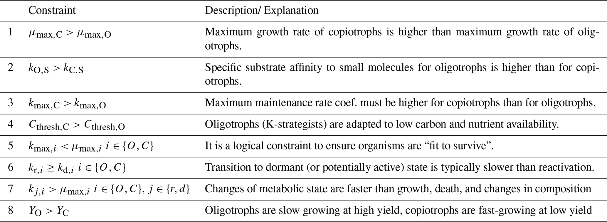
Table G2 Process constraints adapted from the ones defined by Sırcan et al. (2025).

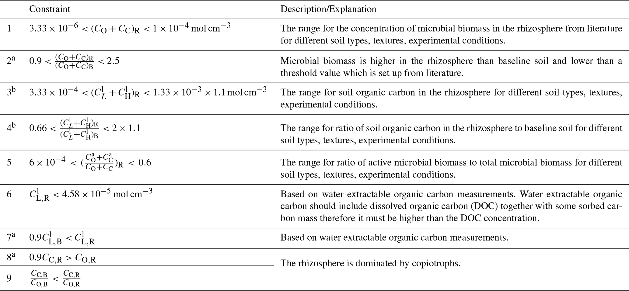
^a The lower bound of the constraint was decreased by 10 % compared with the value defined by Sırcan et al. (2025). ^b The upper bound of the constraint was increased by 10 % compared with the value defined by Sırcan et al. (2025).

Appendix H: Lateral root water conductivity in the mature root zone

The mature root area as well as the root water conductivity (k_lat,x, cm hPa⁻¹ d⁻¹) values for the immature zone are taken from Giraud et al. (2023). However, in that study, $k_{\mathrm{lat},x}=\mathrm{0}$ in the mature root area (more than 0.8 cm away from the root tip). To obtain more realistic results, we used the work of Bramley et al. (2007) to evaluate the $\frac{k_{\mathrm{lat},x,\mathrm{mature}}}{k_{\mathrm{lat},x,\mathrm{immature}}}$ ratio. Bramley et al. (2007, Fig. 4.15) defines the surface-normalised root resistance k_tot,x in m s⁻¹ MPa 10⁻⁸ over the length l (m) from the tip as: $k_{\mathrm{tot},x}\left(l\right)=(-\mathrm{83}\times l+\mathrm{20.9})\times \mathrm{1}\times {\mathrm{10}}^{-\mathrm{8}}$ and the mean root conductance (in in m³ s⁻¹ MPa 10⁻¹¹) as $K_{\mathrm{tot},x}\left(l\right)=(\mathrm{0.7}\times l+\mathrm{2.4})\times \mathrm{1}\times {\mathrm{10}}^{-\mathrm{11}}$. We can therefore obtain the side surface of the root segment (A in m) up to l cm from $A\left(l\right)=\frac{K_{\mathrm{tot},x}\left(l\right)}{k_{\mathrm{tot},x}\left(l\right)}$. Moreover, in their study, the root axial resistance was found to be negligible, and we get therefore $k_{\mathrm{lat},x}\left(l\right)=k_{\mathrm{tot},x}\left(l\right)$ and $k_{\mathrm{lat},x}\left(l\right)=K_{\mathrm{tot},x}\left(l\right)$. We assumed that the mean k_lat,x over the assumed immature root zone could be defined as $k_{\mathrm{lat},x,\mathrm{immature}}\approx k_{\mathrm{lat},x}\left(\mathrm{0.008}\right)$. We then evaluated k_lat,x between l₁=0.07 m from the tip and l₂=0.18 m from the tip, which were the range of distances used in their study. We then computed ${\int }_{l\mathrm{1}}^{l\mathrm{2}}A\left(l\right)\mathrm{d}l$ and ${\int }_{l\mathrm{1}}^{l\mathrm{2}}{k}_{\mathrm{lat},x}\left(l\right)\mathrm{d}l$. From this we could get ${\int }_{l\mathrm{1}}^{l\mathrm{2}}{k}_{\mathrm{lat},x}\left(l\right)\mathrm{d}l=\frac{{\int }_{l\mathrm{1}}^{l\mathrm{2}}{k}_{\mathrm{lat},x}\left(l\right)\mathrm{d}l}{{\int }_{l\mathrm{1}}^{l\mathrm{2}}A\left(l\right)\mathrm{d}l}$. This yielded $\frac{k_{\mathrm{lat},x,\mathrm{mature}}}{k_{\mathrm{lat},x,\mathrm{immature}}}=\frac{{\int }_{l\mathrm{1}}^{l\mathrm{2}}{k}_{\mathrm{lat},x}\left(l\right)\mathrm{d}l}{k_{\mathrm{lat},x}\left(\mathrm{0.008}\right)}\times \mathrm{100}=\mathrm{1.45}\mathit{\%}\approx \mathrm{1.5}$ %. We consequently set $k_{\mathrm{lat},x,\mathrm{mature}}=\mathrm{0.015}{k}_{\mathrm{lat},x,\mathrm{immature}}$ for our modelling study.

Appendix I: Calibration of the soil carbon dynamic

This section describes the method used to calibrate the soil C dynamic. The objective was to implement a simple method allowing us to select sets representing different dynamics. A summary of the characteristics of each of the three selected microbial parameter sets is given in Table 2.

I1 Selection of the microbial parameter sets

In their study, Sırcan et al. (2025) defined 1650 parameter sets for soil model according to a series of parameter and process constraints, which are given in Appendix G. The 1650 parameter sets were divided in three groups according to the resulting gradients of $C_{\mathrm{L}}^{\mathrm{l}}$ directly at the root surface—small, medium, or strong gradient.

• a.

  We randomly selected 33 sets in each of the three gradient categories. Then, we ran the coupled model on the (adapted) parameterised plant of Giraud et al. (2023) between days 10 and 14 of growth (with dynamic soil water and C flows).

• b.

  Sets that did not respect the process constraints defined by Sırcan et al. (2025) were removed–see Table G2.

• c.

  From the 12 remaining sets, we selected three sets representing different soil C dynamics.

For step (a), we ran the simulation without water scarcity effect–meaning, without implementing the effect of water on microbial (de)activation (Eqs. D29, D30) and access to soil solutes (Eq. D10). For step (b), following the method of (Sırcan et al., 2025) and the analysis of Kuzyakov and Razavi (2019), we defined the rhizosphere as the soil volume up to 3 mm from the root surface. The baseline soil (soil outside of the rhizosphere) values were taken from the 3D voxel data at the bottom of the soil column. We retained the sets that respected all the constraints for all the rhizosphere units at the end of the simulation. In some cases, some perirhizal zone units were slightly outside the constraints' bounds. To retain those sets, some constraint bounds were enlarged by 10 %. These bounds-relaxations are indicated in Table G2.

Figure I1 gives the concentration of different C pools along the soil depth. The first set led to a high CO₂ production in spite of a low microbial development, and was named highCO2. The second set led to a high development of the microbial biomass and was named highMB. The last set led to low solute mineralisation and microbial development. It was named lowMUptake.

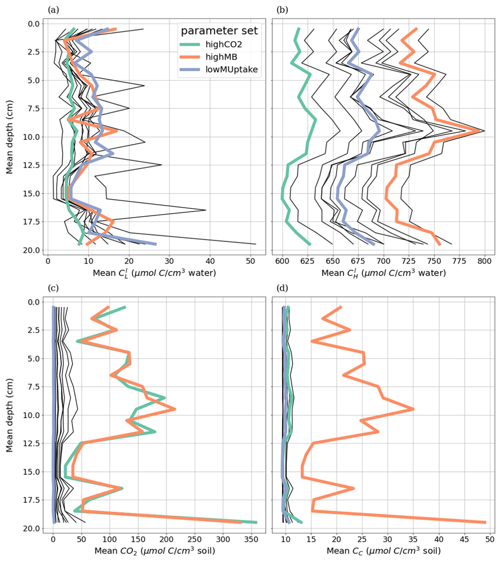
Figure I1 Mean carbon concentration per soil after four days of simulation (day 10 to 14) for concentrations of carbon from high (C_H) and dissolved low ($C_{\mathrm{L}}^{\mathrm{l}}$) molecular weight organic compounds, emitted CO₂, and copiotroph carbon (C_C), in the 3D soil voxels which contain at least one root segment (perirhizal zone). The line colour gives the index of the parameter set. Only parameter sets that respect the process constraints defined by Sırcan et al. (2025) after four simulation days are represented. The selected sets are highCO2 (green line), highMB (orange line) and lowMUptake (purple line).

I2 Description of the selected microbial parameter sets

I2.1 Distribution of the parameter values

Figures I2 and I3 present frequency histograms for each of the parameters in the 1650 sets. The parameters pointed by the numbered arrows correspond to the parameters of the three selected sets (highCO2, highMB, lowMUptake). As we can see, several of the parameter distributions are strongly skewed to the right, making some of the higher values outliers. Therefore, the sets containing the higher parameter values are more likely to give different outputs when compared with the other sets.

From the parameter values, we can give a description of the selected sets:

All three parameter sets offer low β_C (activity of dormant copiotrophs), k_C,S (copiotroph affinity to dissolved low molecular weight organic C compounds), k_d,C, k_d,O (deactivation rates), k_max,C, k_max,O (maintenance rates), μ_max,C, μ_max,O (growth rates), v_max,depoly (depolymerisation rates of high molecular weight organic C compounds) values. This follows the average values of the 1650 sets and lead to a lower microbial activity and slower deactivation. Moreover, the sets have higher than average D_LW values, which should smooth the distribution of $C_{\mathrm{L}}^{\mathrm{l}}$. As can be seen more clearly in Fig. I3, we have an equilibrium between k_d,O and k_r,O: the sets with higher k_d,O also have higher k_r,O. All sets have a higher k_r,C leading to a quick reactivation rate of the copiotrophs. Finally, the three sets have similar $C_{\mathrm{init}}^{\mathrm{l}}$ values, and, in particular, a higher than average $C_{\mathrm{L},\mathrm{init}}^{\mathrm{l}}$.

highCO2 stands out by its higher β_O value, leading to a higher activity for dormant oligotrophs. Moreover, this sets has the higher D_LW values. Finally, the low growth yield (Y_C, Y_O) may lead to higher C usage and CO₂ emission rates.

highMB has higher activation rate parameters (k_r,O, k_r,C) linked with low C_thres parameters, which should lead to a high activated-to-total microbial biomass, although the deactivation parameter for oligotrophs (k_d,O) is also high. The relatively higher affinity parameters (k_C,S, k_O,S) and growth parameters (μ_max,C, μ_max,O) should lead to a quicker increase of the microbial biomass. The low Y (yield parameters) should also lead to higher C usage and CO₂ emissions.

lowMUptake stands out for its low activation rate parameters (k_r,O, k_r,C) linked with high C_thres parameters, which should lead to a high activated-to-total microbial biomass, although the deactivation parameters (k_d,C, k_d,O) are also low. Low maintenance need for dormant microbes (β_C, beta_O) and high yield parameters (Y, Y_C, Y_O) should also lead to a lower C usage and CO₂ emissions.

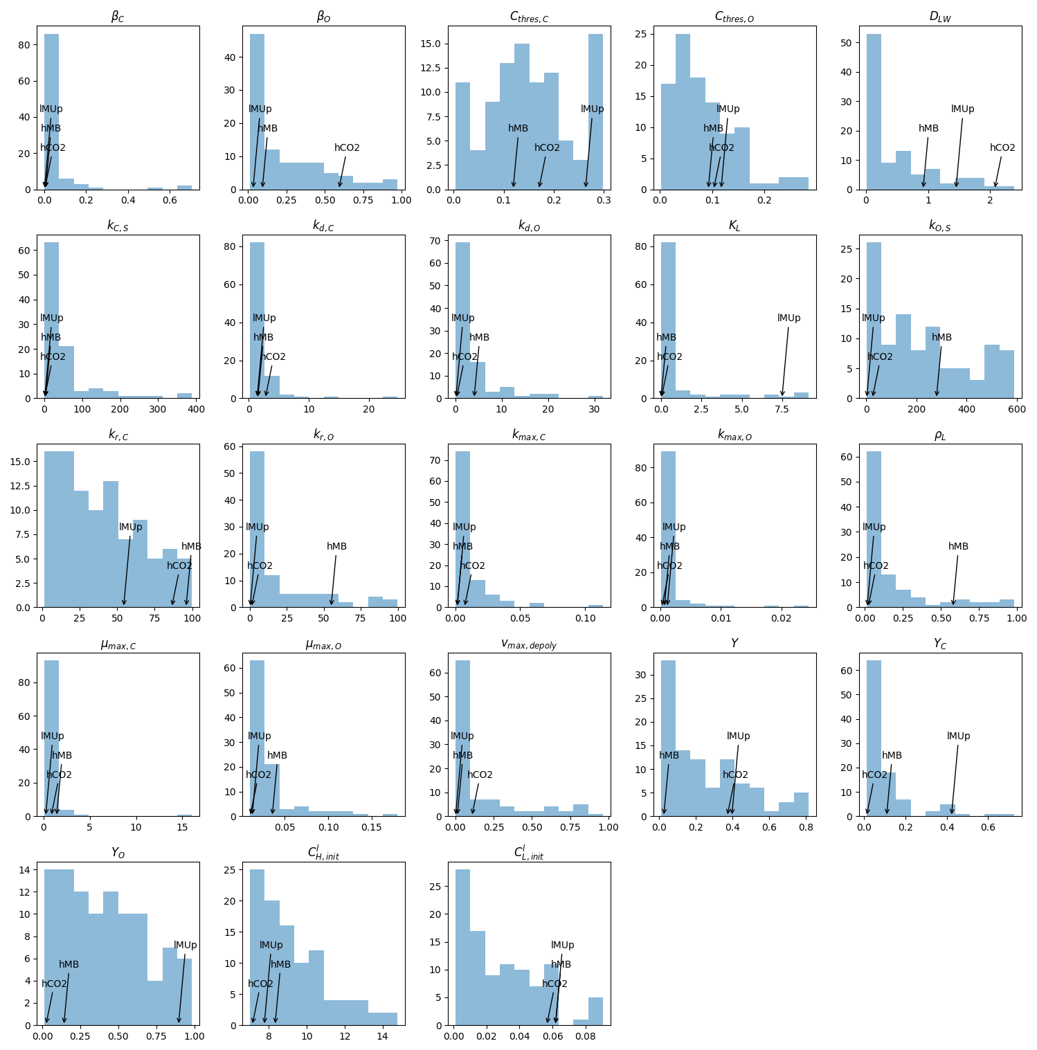
Figure I2 Histogram of the soil input parameters. The parameters pointed by the numbered arrows correspond to the parameters of the three selected sets, highCO2, highMB, lowMUptake, respectively called hCO2, hMB, lMUp.

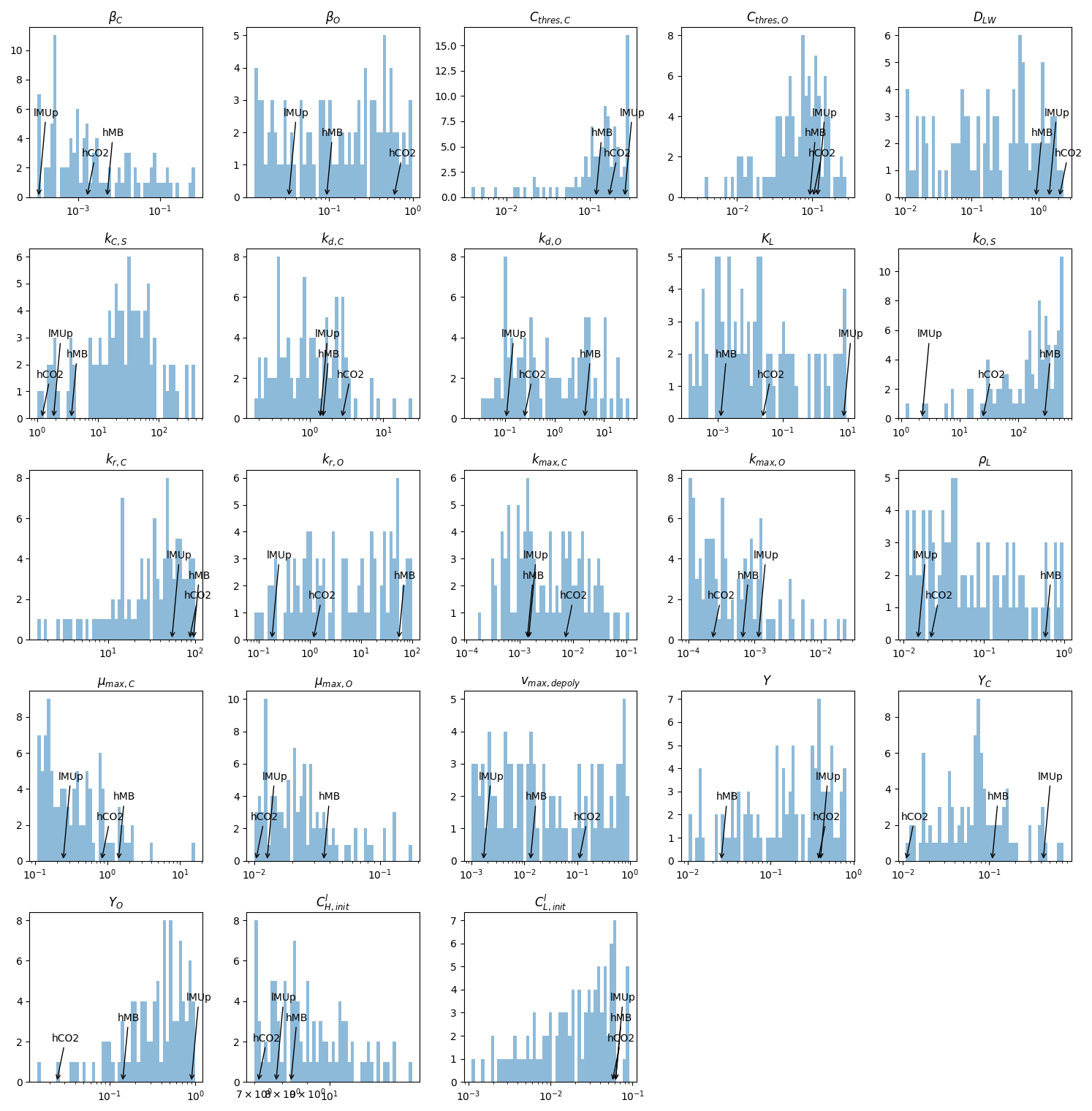
Figure I3 Logarithmic histogram of the soil input parameters. he parameters pointed by the numbered arrows correspond to the parameters of the three selected sets, highCO2, highMB, lowMUptake, respectively called hCO2, hMB, lMUp.

I2.2 Distribution of output variables under different values of dissolved low molecular weight organic carbon

We computed for a range of $C_{\mathrm{L}}^{\mathrm{l}}$ values intermediary outputs describing the microbial dynamic:

• ϕ_O (ϕ_C), –: ratio of oligotrophs (copiotrophs) which will be activated

• S_decay, mol C cm⁻³ d⁻¹: decay rate

• S_growth, mol C cm⁻³ d⁻¹: growth rate

• S_deact, mol C cm⁻³ d⁻¹: deactivation rate of active microbes

• S_react, mol C cm⁻³ d⁻¹: reactivation rate of dormant microbes

• dCO2dt, mol C cm⁻³ d⁻¹: production rate of CO₂

• dMBdt, mol C cm⁻³ d⁻¹: total absolute amount of change in the mass of microbial biomass C per unit of time

Figure I4 give the ratio between the related intermediary variables for all the parameter sets with the selected sets being colored. Figure I5 shows the same data but only for the selected sets. Subgraphics d to i use a logarithmic scale on the y-axis. As we can observe, highCO2 led to a higher relative advantage of the oligotroph compared with the copiotroph regarding their fitness (decay-to-growth rate ratio). This was driven by the higher copiotroph decay-to-growth rate ratio. This was partly compensated by the lower ratio $\frac{S_{\mathrm{growthC}}+S_{\mathrm{decayC}}}{S_{\mathrm{deactC}}+S_{\mathrm{reactC}}}$ indicating that the copiotroph dynamic was more driven by (de)activation than by growth and decay. Moreover, we can note a higher CO₂ emission rate per unit of transformed microbial C.

highMB had lower ϕ values for both copiotrophs and oligotrophs, indicating that lower $C_{\mathrm{L}}^{\mathrm{l}}$ values was necessary for an activation of the microbial community. This led in part to the lower $\frac{S_{\mathrm{deact}}}{S_{\mathrm{react}}}$ for both microbial group, causing a quicker reactivation compared with the deactivation. highMB also led to relatively low decay-to-growth ratio when compared with the other two sets. Finally, for lower $C_{\mathrm{L}}^{\mathrm{l}}$ values, highMB had the highest relative importance of (de)activation on the copiotroph dynamic, when compared with the other two sets. lowMUptake offered the highest copiotroph fitness and the lowest oligotroph-to-copiotroph fitness ratio, giving a relative advantage to the copiotrophs. However, this set had the highest ϕ and $\frac{S_{\mathrm{deact}}}{S_{\mathrm{react}}}$ values, leading to a stronger deactivation of the microbes. For this set, we have a higher importance of the growth and decay over the (de)activation when comparing with the other two sets.

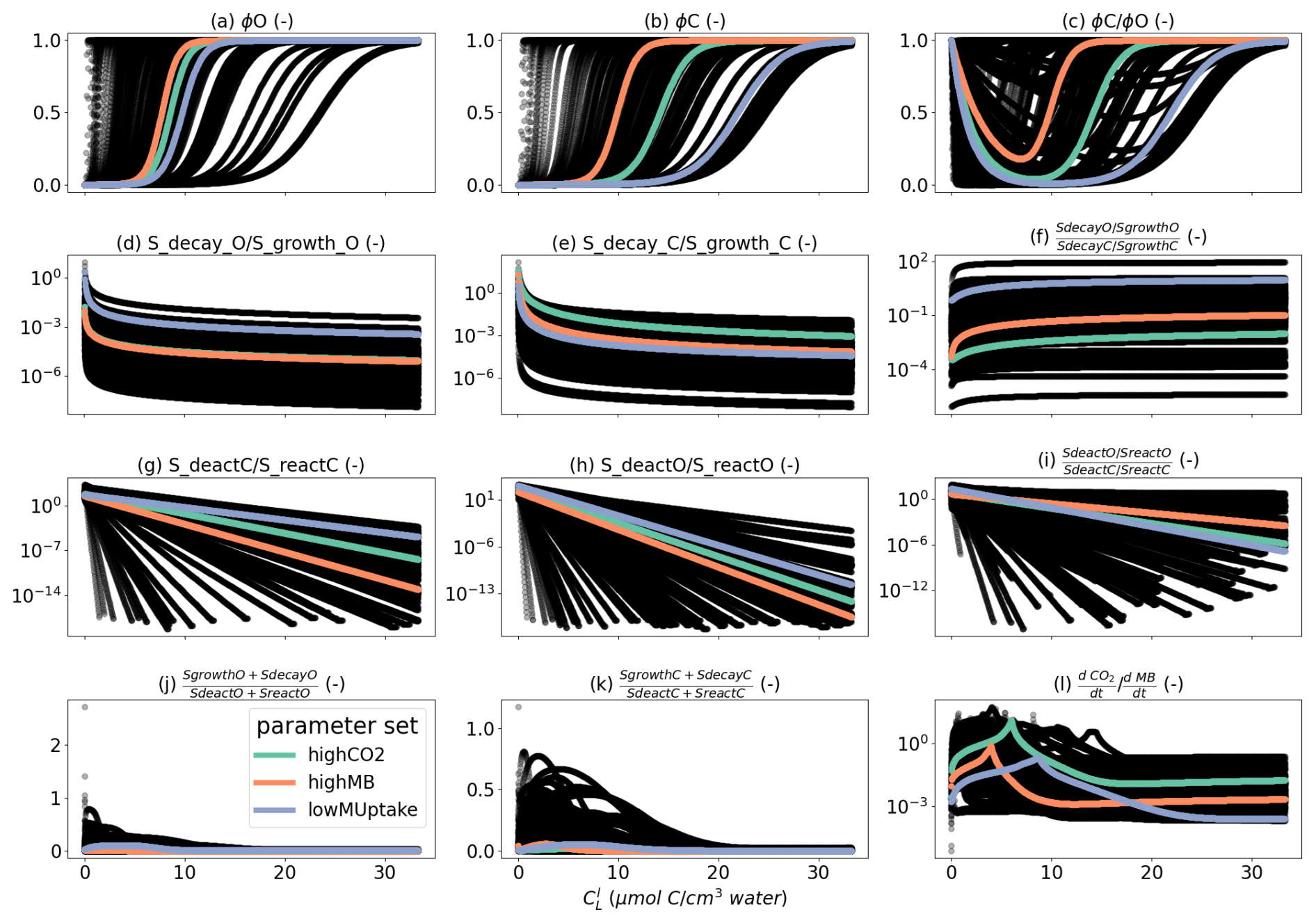
Figure I4 Distribution of specific microbial-related reaction rate for a range of $C_{\mathrm{L}}^{\mathrm{l}}$ for all 99 parameter sets. The coloured values correspond to the three selected sets: highCO2 (green line), highMB (orange line) and lowMUptake (purple line). Graphics (d) to (i) use a logarithmic scale for the y-axis.

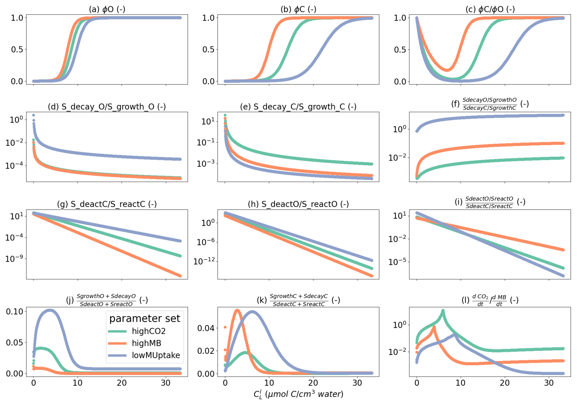
Figure I5 Distribution of specific microbial-related reaction rate for a range of $C_{\mathrm{L}}^{\mathrm{l}}$ for the selected parameter sets. The coloured values correspond to the three selected sets: highCO2 (green line), highMB (orange line) and lowMUptake (purple line). Graphics (d) to (i) use a logarithmic scale for the y-axis.

Appendix J: Selected scales for the simulation outputs

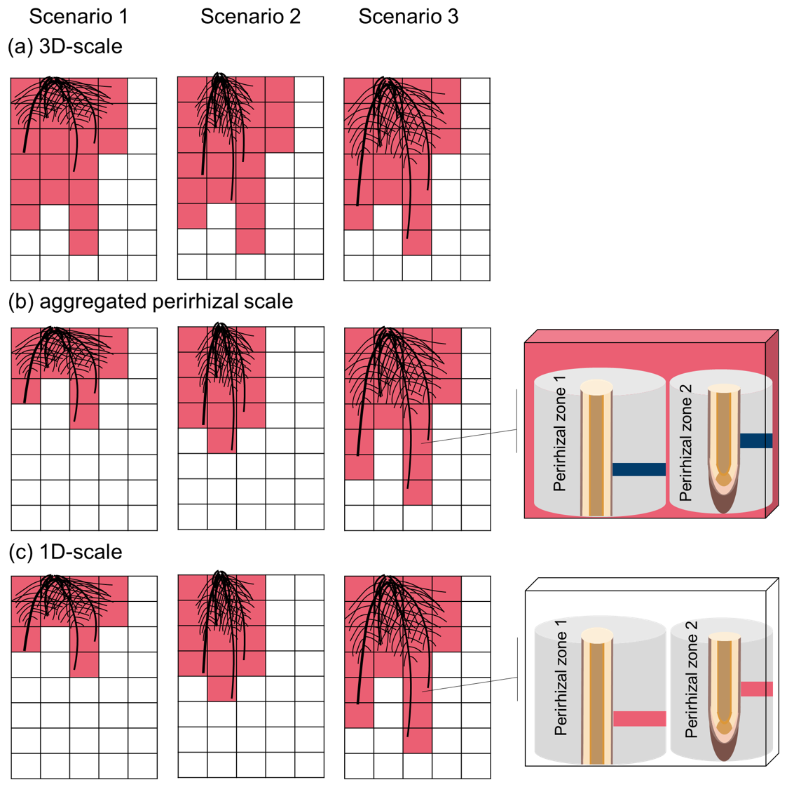
Figure J1 Graphical representation of the three scales used to analyse the simulation outputs in the main body of the text, using three example scenarios. (a) The 3D scale includes all the 3D voxels that contain at least one root at one time step of the simulations in any of the scenarios. This volume is constant over time. (b) The volume if the aggregated perirhizal scale can change at each time step and between scenarios. It includes the 3D voxels that contain at least one root for the studied time point of the studied scenario. (c) The 1D scale includes all the sub-control volume of the the 1D soil model for the studied time point of the studied scenario. The 1D scale covers the same area as the aggregated perirhizal volume but represent a higher resolution: one data point for each sub-control volume of the 1D-models, against one data point for each sub-control volume of the selected 3D soil voxel. The definition of the perirhizal_trunc presented in the appendix is not included in this graphic.

Appendix K: Complementary results

K1 Model runtime

The model was implemented on the Institute of Bio- and Geosciences (IBG-3) computer cluster, Forschungszentrum Jülich. Each simulation was run on one node (shared memory) and 32 cores (Mainboard Supermicro H12DSU-iN), using all 32 cores for the simulation of the 1D and 3D soil domains and one core for the plant domain. The run-time of the simulation lasted between 9 h (baseline with highSolutes) and 13 h (lateDry with highCO2). The time step of the fixed point iteration remained at 20 mn for the baseline scenarios, went several times down to 7 mn for the earlyDry and lateDry scenarios. The computation of the water flows and content was the main bottleneck for the convergence of the iteration loop. For baseline, respectively 17 %, 10 %, and 27 % of the runtime was spent solving the 3D soil domain, 1D soil domain, and plant models. For earlyDry, on average, 36 %, 9 %, and 14 % of the runtime was spent solving the 3D soil domain, 1D soil domains, and plant models. For lateDry, on average, 38 %, 11 %, and 15 % of the runtime is spent solving the 3D soil domain, 1D soil domain, and plant model. In total, between 54 % and 64 % of the runtime was dedicated to solving the models.

K2 Normalised root length density

K3 Plant processes

Figure 7A presents the plant xylem mean water potential (ψ_x, cm) for each kinetic parameterisation and weather scenario. The simulation results reflect the diurnal dynamics of the xylem water potential in response to the truncated sinusoidal curve used to describe the atmospheric conditions (light input, air relative humidity and temperature). These boundary conditions affected the plant stomatal regulation and, thus, the C assimilation and transpiration rate. We observed an increase of the xylem water potential over time for baseline as the leaf : root ratio decreased. With drought, the xylem water potential rapidly decreased at the beginning of the dry spells and recovered after its end in response to changes in soil water content and mean air relative humidity during the dry spells (see Table 1). Towards the end of the simulation with earlyDry, the xylem water potential converged to the values of baseline, indicating a full recovery of the plant water uptake capacity. As a consequence of the lower leaf : root ratio, the xylem water potential was lower at the beginning of the dry spells for earlyDry (11th day) than for lateDry (18th day). However, in comparison to earlyDry, the higher plant transpiration under lateDry with higher total leaf and root surface area led to a quicker decrease in soil water content. This mechanism induced lower xylem water potential in the lateDry compared to the earlyDry scenario from the third day after the start of the dry spells onward (13th and 20th day).

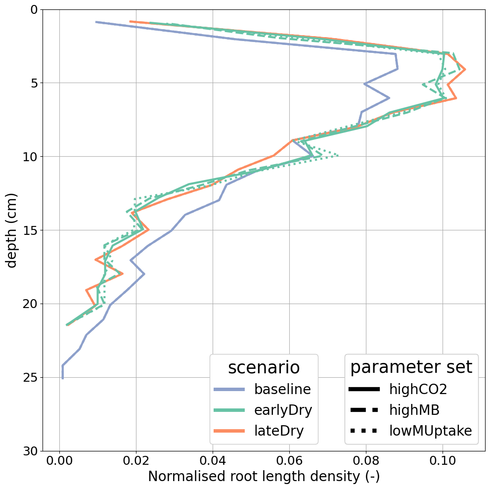
Figure K1 Normalised root length density at the end of the simulation. Line colours indicate the weather scenarios: baseline (blue) against an early (green) and late (red) dry spell. Line types represent different kinetic parameter sets.

Figure 7B shows the cumulative amount of C used for growth (and growth respiration) during the simulation. The diurnal cycle of the xylem water potential affected the plant growth. During the day, the transpiration-induced lower xylem water potential limited plant growth compared to the night, where increased xylem water potential permitted faster, albeit still water-limited, C assimilation and biomass production. The required C was taken from the starch reserves built up during the day. We can also observe trends over the simulation. Unlike younger plants, older plants could maintain growth during the diurnal period outside of the dry spells. During the dry spells, growth occurred only at night and at a severely reduced rate. On the last three nights of the late dry spell, we observed no night-growth due to lower plant night xylem water potential.

Plant maintenance respiration increased during the spells due to the higher air temperatures. In the earlyDry scenario, plant growth was severely limited compared to baseline, resulting in a lower plant maintenance respiration rate after the dry spell ended (18th day). For lateDry, we saw a lower maintenance respiration rate from the fourth day of the spell. The total cumulative respiration (growth and maintenance related) at the end of the simulation was highest for the baseline scenario. It was about 29 % lower for earlyDry and 18 % lower for lateDry. The kinetic parameterisation had no significant effect on the plant water processes or growth and maintenance. Simulation results indicate that plant expansion growth is strongly influenced by changes in water potential during the diurnal cycle and drought periods, consistent with processes described in previous studies (Verbančič et al., 2018; Barillot et al., 2020; Coussement et al., 2018; De Swaef et al., 2022). However, it is hypothesised that cell wall biosynthesis (biosynthetic growth) predominantly occurs during the day using photoassimilates, while being much more limited at night when it relies on starch reserves (Verbančič et al., 2018). The expansion growth corresponds to the dilatation of those walls, driven by the cell’s turgor pressure. Therefore, expansion growth depends on the supply of C but does not need to be concurrent to C supply. For this simulation, the virtual plant’s starch pool, which varied according to the C supply, can be interpreted as representing both actual starch reserves and newly synthesised wall material. The carbon belonging to the newly synthesised wall material was moved to the carbon used for growth once these walls undergo expansion growth, thereby enabling the expansion growth to occur at night. To achieve robust results and better recreate typical C dynamics across a wider range of parameter sets, it could be beneficial to explicitly represent biosynthetic growth in future models. Following the analyses of Verbančič et al. (2018) and Barillot et al. (2020), high biosynthetic growth requires higher C supply but results in the creation of new cells more flexible and capable of expanding under lower turgor pressure. This higher amount of cells with high cell wall flexibility can help maintain plant growth in case of drought (Blum, 2017). Another mechanism supporting growth under low turgor pressure is osmotic adjustment, which has been identified as a critical process during drought conditions (Blum, 2017; Coussement et al., 2018). Not including this process in our model could explain the high growth limitation caused by drought observed in our simulation.

In spite of these limitations, the outputs of these study follow more closely experimental results than those of Giraud et al. (2023): expansion growth occurring at night, starch supply and exudation being the regulatory variables for plant carbon balance.

Appendix L: Complementary cumulative volume distributions

For the perirhizal_trunc analysis, we aggregated the mean concentrations for each 1D domain truncated at a specified distance from the root surface, denoted as Δr_analysis. The value of Δr_analysis was pragmatically set to 0.06 cm. It corresponds to the minimum distance between the inner and outer boundaries of the 1D domains obtained during the simulation. By setting a consistent distance between the inner and outer boundaries of the truncated domains, we obtained a partial uniformity between the domains that reduced variations that could arise from differences in soil allocation to each domain (see Eq. 26). Moreover, using these truncated 1D models allowed us to evaluate a soil area nearer to the root surface, for comparison with the aggregated perirhizal scale.

We created complementary cumulative volume distribution plots of the concentration at the perirhizal_trunc scale. In these plots, the x-axis represents different concentration values. The y-axis shows the absolute or relative volume of the selected perirhizal zone (up to 0.06 cm from the root surface) with concentrations equal to or greater than the corresponding x-axis value. This representation provides insight into the spatial variability and distribution of concentrations within the specified zone. Additionally, these graphs allow us to evaluate how much of the perirhizal zone volume exceeds certain concentration levels, such as hotspot thresholds.

Figure L1 shows the perirhizal_trunc volume with a concentration inferior or equal to the value on the x-axis. The description and motivation of the evaluation method for this figure are given in Sect. 2.4.3. A video presenting this graphic for each time step is available at https://doi.org/10.5446/72786 (“Video S1”, Giraud, 2026a). Root exudation and mucilage release triggered concentration peaks of solutes and microbial C in the perirhizal_trunc volume (Fig. L1). Particularly copiotrophs were strongly stimulated reaching high abundances up to 580 µmol (cm³ soil)⁻¹ for lateDry with highMB, for a volume of $\mathrm{2.9}\times {\mathrm{10}}^{-\mathrm{2}}$ cm. Both dry spells led to strongly reduced total perirhizal_trunc volumes at the end of the simulation of 42 % for earlyDry and 34 % for lateDry in relation to baseline. As a consequence, maximum concentrations of high molecular weight organic compounds-C and copiotrophs-C concentrations were lowest with baseline because the released plant C triggering copiotrophic growth was distributed in a larger volume.

While lateDry with highCO2 and highMB caused the highest CO₂, copiotrophs-C and dormant copiotrophs-C peaks at the aggregated perirhizal scale (see respectively Figs. 8, 9), for the perirhizal_trunc zone the highest values for these parameter sets were obtained with earlyDry (Fig. L1c, d, f). The simulated copiotroph growth during the dry spell occurred earlier under earlyDry, creating a larger pool of dormant copiotrophs-C ready to be re-activated and grow during periods of high exudation. As the growth rate is a function of the current active copiotrophs-C, high dormant copiotrophs-C early in the simulation favoured the overall growth in those hotspots.

Parameterizing the model with highMB under lateDry caused an especially high copiotrophs-C over most of the perirhizal_trunc volume with an increase of active and a strong build-up of dormant copiotrophs (Fig. L1d, e, f). Conversely, although highMB under lateDry also led to a slight increase in the total and dormant oligotrophic concentrations (Fig. L1g, i), it resulted in a decrease in the amount of active oligotrophs (Fig. L1h). This simulated pattern indicates a pronounced competition between oligotrophs and copiotrophs for this scenario-parameter set combination. Indeed, the active oligotrophs-C values started decreasing strongly during the second half of the late dry spell, when the exudation rate became also lower.

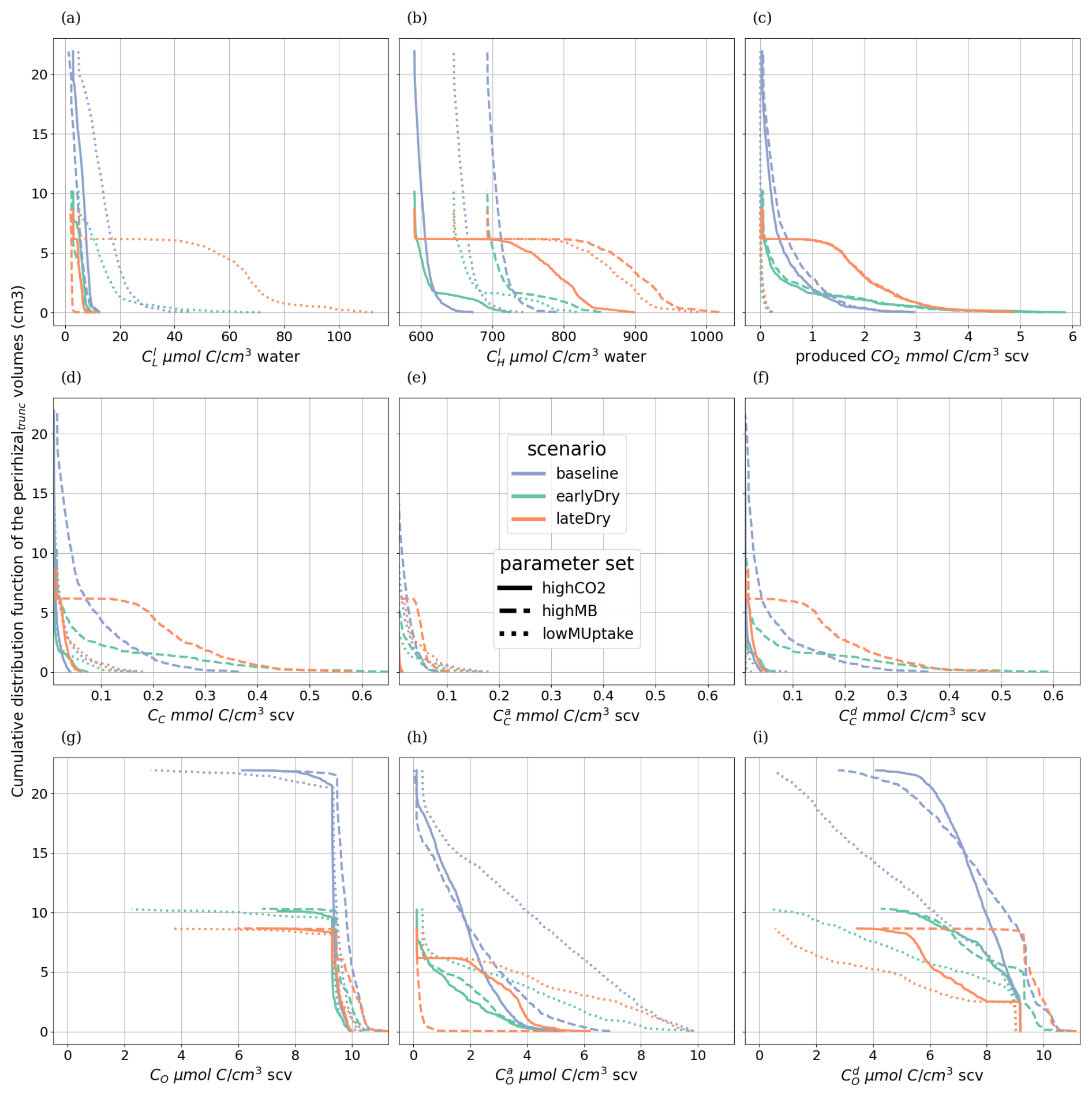
Figure L1 Perirhizal zone volume according to the minimal concentration of organic carbon in the truncated perirhizal zones, for (a) carbon of low-weight dissolved organic molecules ($C_{\mathrm{L}}^{\mathrm{l}}$), and (b) carbon of high-weight organic molecules (C_H), (c) emitted CO₂, (d) total (C_C) (e) active ($C_{\mathrm{C}}^{\mathrm{a}}$) (F) dormant ($C_{\mathrm{C}}^{\mathrm{d}}$) copiotrophs in the soil phase, (g) total (C_O) (h) active ($C_{\mathrm{O}}^{\mathrm{a}}$) (i) dormant ($C_{\mathrm{O}}^{\mathrm{d}}$) oligotrophs in the soil phase. The line colors give the weather scenario: baseline (blue) against an early (green) and late (red) dry spell. The line types represent the different kinetic parameterisation. Subplots (d), (e), (f) and (g), (h), (i) have the same scale on the x-axis.

Appendix M: Radial carbon concentration profiles

To evaluate how the concentration of low-weight dissolved organic molecules-C is linked with the development and activation of the most important microbial pool (copiotrophs), Fig. M1 presents the radial concentration profile of the copiotrophs-C and atcive-to-total copiotrophs-C ratio at the end of the simulations. We observed a very steep gradient of copiotrophs-C according to the distance from the root surface for highMB and highCO2. Indeed, the microbes developed around the C source. As they were not motile, they remained on this segment even once the root segment had become older and its C releases and water uptake decreased. For lowMUptake, the copiotrophs-C gradient (like the low-weight dissolved organic molecules-C concentration gradient, see Fig. 12) was smoother than the other two parameter sets for all weather scenarios. Therefore, even though copiotrophs-C directly at the root-soil interface is higher with highCO2 than with lowMUptake, we observed similar copiotrophs-C values at the aggregated perirhizal scales (Fig. 9).

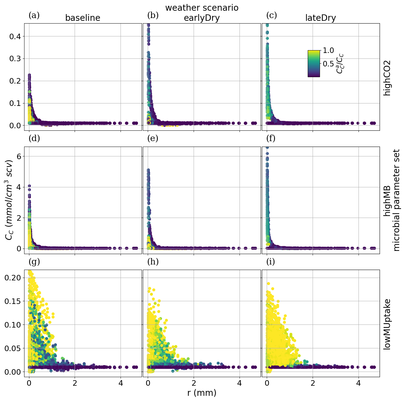
Figure M1 Radial concentration profile of copiotroph carbon at the end of the simulation for each plant perirhizal zone. r (mm) corresponds to the distance to the root surface. The colour gives the ratio of active-to-total oligotroph biomass. Each column corresponds to a specific weather scenario and each row corresponds to a specific kinetic parameterisation. We have a different y-axis for each row.

M1 Effects of drought in the bulk soil

To better understand the effect of drought on the perirhizal zone, Fig. M2 presents the relative change of carbon allocation caused by the droughts in the bulk soil. To represent the bulk soil, we selected the soil voxels at the bottom of the simulated soil column, which were separated by the nearest root by over 13 cm. We can observe that the relative changes in carbon allocation was much more limited than within the perirhizal zone, and less affected by the day-night cycle. The lower soil water content allowed for a higher concentration of soil solute, which led to a higher activation of the soil microbes (Fig. M2a). However, the lower soil water potential also slowed the microbial activity, leading to a lower uptake of resources (Fig. M2d), CO₂ emissions (Fig. M2c), and microbial growth (Fig. M2b). At this distance from the roots, the microbes are not affected by the changes in plant C releases, which lowers the differences between the earlyDry and lateDry scenarios.

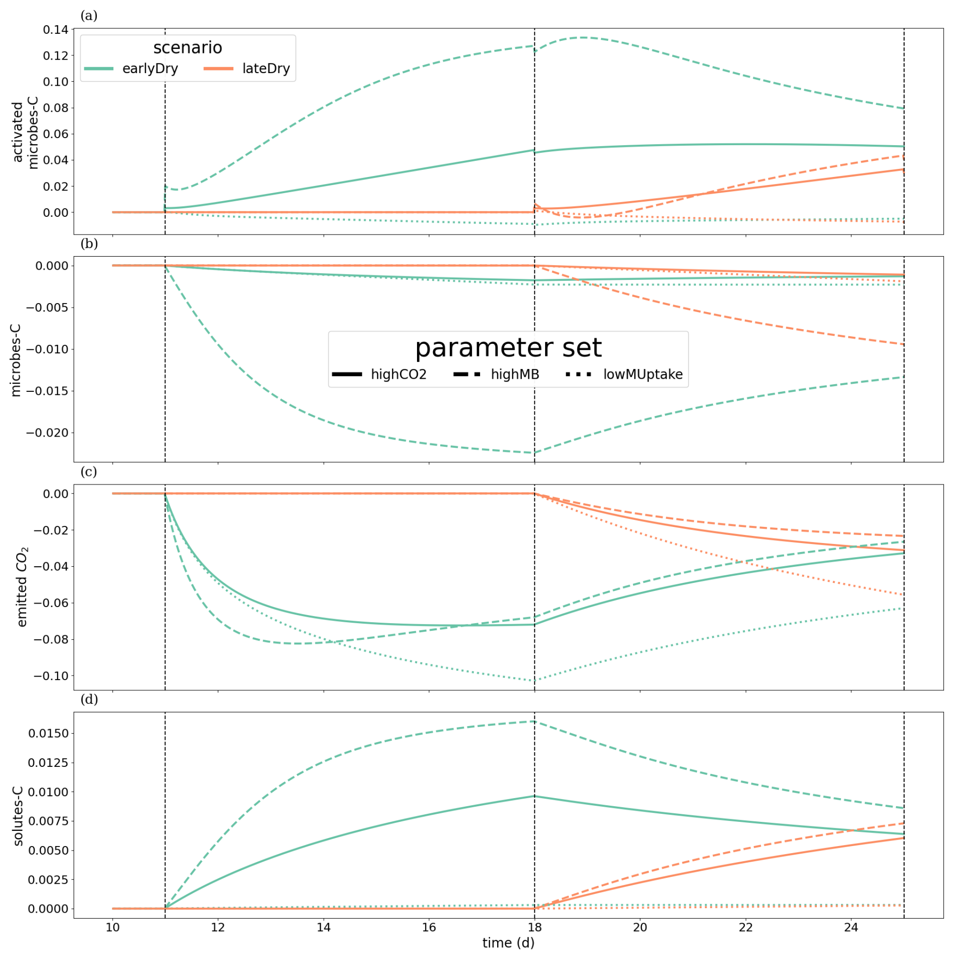
Figure M2 Relative change of carbon allocation in response to drought scenarios according to the kinetic parameters in the bulk soil. The panels present the difference of C between each drought treatment and the baseline in relation to the baseline C usage for (a) microbes-C, (b) activated microbes-C, (c) CO₂ emitted by microbes, (d) soil solutes-C. The line types represent the different kinetic parameterisation. The dotted lines show the beginning and end of the early (day 11 to 18) and late (day 18 to 25) dry spells. Please note that the scales of the y-axis differ in each subplot.