Using 3D observations with high spatio-temporal resolution to calibrate and evaluate a process-focused cellular automaton model of soil erosion by water

Future global change is likely to give rise to novel combinations of the factors which enhance or inhibit soil erosion by water. Thus, there is a need for erosion models, necessarily process-focused ones, which are able to reliably represent the rates and extents of soil erosion under unprecedented circumstances. The process-focused cellular automaton erosion model RillGrow is, given initial soil surface microtopography for a plot-sized area, able to predict the emergent patterns produced by runoff and erosion. This study explores the use of structure-from-motion photogrammetry as a means to calibrate and evaluate this model by capturing detailed, time-lapsed data for soil surface height changes during erosion events.

Temporally high-resolution monitoring capabilities (i.e. 3D models of elevation change at 0.1 Hz frequency) permit the evaluation of erosion models in terms of the sequence of the formation of erosional features. Here, multiple objective functions using three different spatio-temporal averaging approaches are assessed for their suitability in calibrating and evaluating the model's output. We used two sets of data from field- and laboratory-based rainfall simulation experiments lasting 90 and 30 min, respectively. By integrating 10 different calibration metrics, the outputs of 2000 and 2400 RillGrow runs for, respectively, the field and laboratory experiments were analysed. No single model run was able to adequately replicate all aspects of either the field or the laboratory experiments. The multiple objective function approaches highlight different aspects of model performance, indicating that no single objective function can capture the full complexity of erosion processes. They also highlight different strengths and weaknesses of the model. Depending on the focus of the evaluation, an ensemble of objective functions may not always be necessary.

These results underscore the need for more nuanced evaluation of erosion models, e.g. by incorporating spatial-pattern comparison techniques to provide a deeper understanding of the model's capabilities. Such calibrations are an essential complement to the development of erosion models which are able to forecast the impacts of future global change. For the first time, we use data with a very high spatio-temporal resolution to calibrate a soil erosion model.

1 Introduction

Soil erosion by water is an environmental problem of global significance (e.g. Nearing et al., 2017; Quinton and Fiener, 2024). In the future, it is likely to become more pressing in locations where anthropogenically driven climate change brings about more and/or more intense rainfall and/or where changes in land usage (resulting from changes in climate, economic factors, and/or other drivers) operate to leave soil unprotected by vegetation during times of heavy rainfall (e.g. Boardman et al., 1990; Favis-Mortlock and Boardman, 1995; Li and Fang, 2016; Dunkerley, 2019; Chen et al., 2024; Zhao et al., 2024). Such future changes are likely to result in novel combinations of the factors which cause or inhibit erosion (Foucher et al., 2024).

To manage soil erosion by water, quantification of the rate and extent of erosion is essential. Modelling is a primary tool for such quantification. However, when aiming to model erosion under novel circumstances, it is unwise to make use of models which work in a wholly “black-box” manner, that is by extrapolating from previously encountered combinations of erosion-causing and/or erosion-inhibiting factors. Such models (e.g. Wischmeier, 1976; Renard et al., 1991; Panagos et al., 2015) cannot represent the impacts upon erosion rates and extents due to currently unknown thresholds of or non-linearities in the response to the erosion-causing and/or erosion-inhibiting factors. It is these thresholds and non-linearities which will provide the greatest surprises with regard to future erosion. Thus, there is a vital scientific need to improve and to continue to improve our understanding of the processes of soil erosion by water and to incorporate this understanding into quantitative process-focused models, with (at the same time) such models ideally making use of readily available data sources. This is a considerable challenge, but only by doing this will we be able to satisfactorily manage future soil erosion by water.

While there are many process-focused models which simulate the effects of soil erosion by water (e.g. Jetten et al., 1999; Batista et al., 2019; Raza et al., 2021; Rose and Hadaddchi, 2023), the RillGrow model (Favis-Mortlock, 1998) is unusual in its adoption of a cellular automaton (CA: see “List of abbreviations” in the Appendix) representation of the eroding soil surface (cf. Smith, 1991; Murray and Paola, 1997; Coulthard et al., 2002; Darboux et al., 2002; Nicholas, 2005). CA models have been used to study emergent phenomena in a wide variety of scientific domains (e.g. Wolfram, 1984; Wu, 1998; Cappuccio et al., 2001; Wahle et al., 2001; Silva et al., 2019; Favis-Mortlock, 2004). In RillGrow – as in the majority of CA models – all process interactions are “local”, i.e. take place only between adjacent cells of the digital elevation model (DEM) grid which represents soil surface elevations (and other soil properties). There are no process representations which operate in the DEM as a whole. As a consequence of this purely local focus, the model makes no distinction between rill and inter-rill erosion processes. Instead, they are considered to be part of a continuum. The model's local (i.e. confined to a single cell and the cells which surround it) representation of erosion processes creates larger emergent multi-cell patterns: micro-rills and rills (Favis-Mortlock et al., 2000).

As with virtually all erosion models (e.g. Favis-Mortlock et al., 2001), there is a need to calibrate the empirical inputs which RillGrow requires and then to evaluate model results against observations (Jetten et al., 1999; Batista et al., 2019). The relatively unusual modelling approach adopted by RillGrow lends itself to the exploitation of novel tools for calibration (Epple et al., 2022). This is particularly so with regard to the capturing of spatial patterns, such as rill networks.

In an early RillGrow study (Favis-Mortlock, 1998), a moving-head laser scanner was used to capture microtopography: first of the initial soil surface of a laboratory-based plot and then of the eroded soil surface of the plot following simulated rainfall. The initial-surface DEMs which resulted from these scans were used as inputs for RillGrow, and the end-of-experiment DEMs were used to evaluate the model's output. However, this strategy – comparing the model's spatial output only with the end-of-experiment DEM – leaves open the possibility of “the right answer for the wrong reason” since modelled rills may form in a temporal sequence which is different from reality. The sequence with which erosional channels are incised (i.e. the dynamic development of flow-routing patterns) is of major importance when considering temporal changes in connectivity for areas ranging from plot-sized to field-sized (Baartman et al., 2020).

Thus, there is a need for intra-experiment DEM captures (time slices) to improve model evaluation. A subsequent laboratory-based RillGrow study used data from Helming et al. (1998) and did make use of intra-experiment DEMs. However, it was necessary to pause the simulated rainfall in order to use the laser scanner to capture the intra-experiment microtopography and then to restart the simulated rainfall. These within-experiment pauses were necessary for two reasons: firstly, because laser scanning could not be carried out with simulated rain falling onto the moving scanner head (and even if it could, the scanner head would interfere with the uniformity of the simulated rain) and, secondly, because laser scanning as used in this experiment was not instantaneous, with the laser scanner rather requiring some minutes to cover the whole plot area. Pausing an experiment in this way to capture a snapshot of rapidly changing microtopography is potentially problematic. Diminishing flow in rills during intra-experiment stoppages will result in within-rill deposition, which may influence subsequent within-rill detachment when rainfall is restarted; also, a newly developed soil crust (or seal) may begin to dry out and so change its properties, particularly with regard to infiltration.

Another RillGrow study (Favis-Mortlock et al., 1998) made use of simple photogrammetry to capture initial and final DEMs of a small area together with a single intra-experiment DEM which was obtained without pausing the experiment. Whilst this was a step forward, a single intra-experiment DEM is not enough to satisfactorily evaluate the temporal sequence with which erosional patterns form; also, there were problems with raindrops obscuring parts of the eroding area.

Structure-from-motion (SfM) photogrammetry can easily capture multiple intra-experiment DEMs because almost all processing is automatic (Eltner and Sofia, 2020); it therefore promises to be a useful tool in calibrating spatially explicit erosion models such as RillGrow. SfM photogrammetry permits intra-experiment measurements of changes in soil surface microtopography at millimetre to centimetre resolutions for plot- and hillslope-sized areas, with millimetre to centimetre accuracy (e.g. Eltner et al., 2018; Hänsel et al., 2016). So far, SfM photogrammetry in the field of erosion studies has mainly been applied to unoccupied aerial vehicle (UAV) imagery. However, its potential for application with terrestrially installed camera systems to increase the frequency of geomorphic change detection to hours (e.g. Blanch et al., 2024) or even to seconds (Eltner et al., 2017) has been illustrated. Note that, with time-lapse SfM photogrammetry, falling raindrops obscuring the plot or hillslope are less of an issue (unlike in the approach used in Favis-Mortlock et al., 1998) due to the high frequency of capturing data and, thus, the increased likelihood of capturing images during rainfall gaps.

For model calibration and evaluation, the most commonly used approach involves space–time averaging: a simple comparison of measured and modelled runoff and sediment yield at the end of the plot (or at the catchment outlet) and at the end of the period of observation. Sometimes, this is supplemented by comparisons of measured and modelled time series, constructed from additional plot-end (or catchment outlet) measurements during the period of observation. There have been attempts to evaluate erosion models using spatial data, e.g. from field surveys, aerial images, and fallout radionuclide data (Brazier et al., 2001; Fischer et al., 2018; Jetten et al., 2003; Saggau et al., 2022; Vigiak et al., 2006). However, it has been and still is much less common to compare the measured and modelled spatial patterns of erosion. It is even less common to do so using more than one method for comparison.

From the perspective of the historical development of erosion models (e.g. Nicks, 1998) it is unsurprising that model evaluations have concentrated on simple spatio-temporal averaging approaches. The USLE (Wischmeier, 1976) and subsequent models based upon the USLE (e.g. MUSLE: Williams, 1975; RUSLE: Renard et al., 1991; USLE-M: Kinnell and Risse, 1998) are only capable of generating results which are averaged over both time and space. Subsequent, more process-focused erosion models such as WEPP (Nearing et al., 1989) or Erosion-2D (Schmidt, 1991) introduced a 2D spatial element: a hillslope profile. Later came models with an explicit spatial focus, such as LISEM (de Roo et al., 1996) and Erosion-3D (Schmidt, 1996). The evaluation of erosion models has therefore lagged behind the development of the models themselves.

The aims of this study were, first, to use several multiple objective functions to calibrate a process-focused soil erosion model (RillGrow) and then to evaluate these objective functions in terms of information gained from each function. We used time-lapse SfM photogrammetry and measured the sediment yield from two plot-sized rainfall simulations, one in the field and the other in the laboratory. Ten different objective functions were considered to calibrate model parameters. The best-performing model runs were chosen to be those with the lowest residuals for multiple objective functions. This novel approach to testing erosion models considers both 3D models of change with high spatio-temporal resolutions and multiple sediment yield measurements at the plot outlet.

2 Methods

2.1 Data acquisition

The field and laboratory rainfall simulators of the Czech Technical University in Prague were used in this study (Fig. 1). Rainfall simulators can both control several characteristics of incident raindrops and accelerate erosion processes for a faster monitoring of soil surface changes. Thus, simulators have become an integral part of erosion research, including erosion model calibration and evaluation (Iserloh et al., 2013; Prosdocimi et al., 2017; Bosio et al., 2023).

Figure 1 Rainfall simulator used in the field (a) and in the laboratory (b).

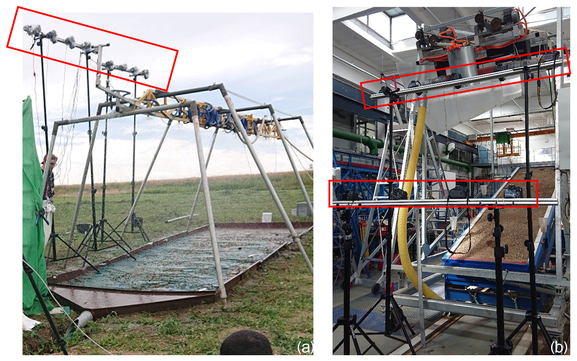
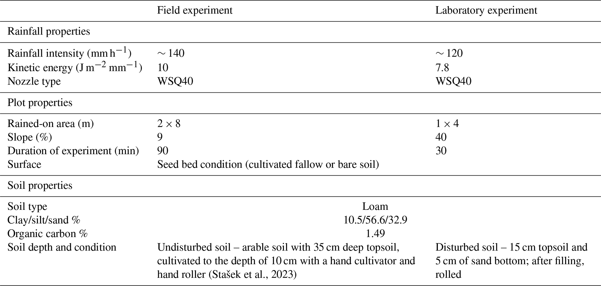
During the field experiment, the rainfall simulator (Kavka et al., 2018) was used on a plot that had been prepared as cultivated fallow. For the laboratory experiment, the rainfall simulator (Kavka et al., 2019) was used on a disturbed soil sample which had been prepared similarly to the field experiment. Further site and experiment properties are given in Table 1.

Table 1 Rainfall, plot, and soil characteristics for both field and laboratory rainfall simulation experiments.

Both rainfall simulation experiments used the same approach with regard to runoff and sediment sampling: a standard procedure described by Stašek et al. (2023). At the bottom of the plot, runoff is routed into a metal funnel. Samples are collected at volumes of 1 to 2 L every 2.5 min after the start of runoff. Samples were weighted to obtain the volume of surface runoff and then were filtered using KA-3M paper filters (Papírny Pernštejn, Czechia) and dried at 105 °C in an air drier in order to obtain the amount of soil per sample.

Nine single-lens reflex (SLR) cameras (Canon EOS 450D, 600D, 1100D, and 2000D and Nikon D700) were used to create the photogrammetric data for both the field and the laboratory experiments (Fig. 2). These captured images every 10 s in a synchronized manner using a remote trigger which had been constructed in-house. The cameras used different but fixed focal lengths to ensure a stable principal distance during the experiment. At the field site, the cameras were mounted at a height of about 4 m. This captured a region of interest (RoI) of about 4 m², covering the lower part of the plot. In the laboratory, the whole plot could be captured (about 4 m²). Images were also captured with a Sony Alpha 6600 (142 and 148 images at the field site and 77 and 79 images in the laboratory before and after the experiment, respectively) by walking around the plot to measure the entire area underneath the rainfall simulator. Ground control points (GCPs) were distributed around the plot (15 and 22 for the field and laboratory experiments, respectively) and measured with millimetre accuracy using a total station in order to scale and reference the image measurements.

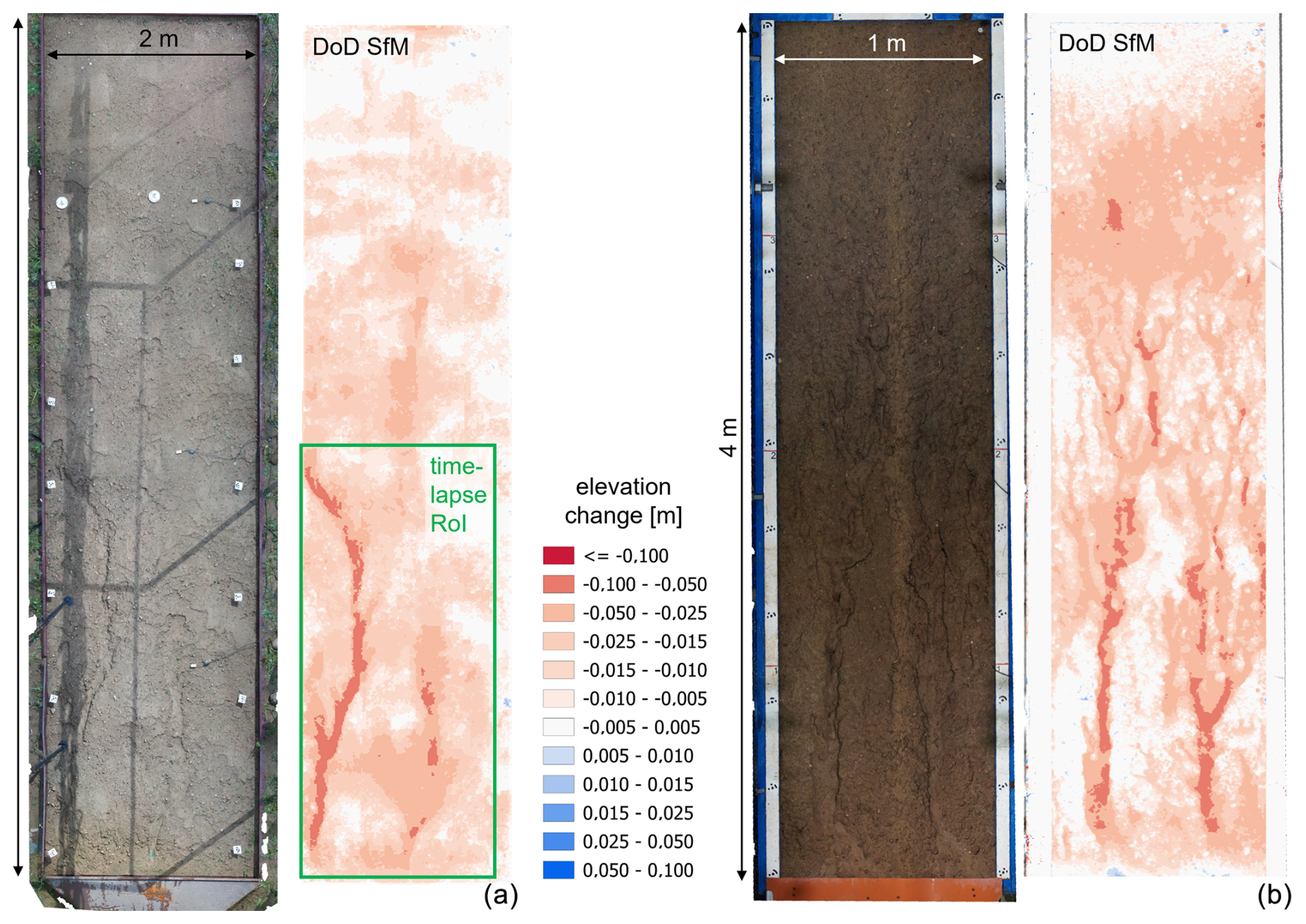
Figure 2 Ortho photo (left) and elevation change map (right) of the field (a) and laboratory (b) experiments. The cameras for time-lapse SfM are marked with red boxes. The green box in (a) shows the region of interest, for which high-temporal-resolution change observations were made.

2.2 Image data processing

Images captured with the Sony Alpha 6600 were used to derive 3D representations of the whole plot for both the field and the laboratory experiments using Agisoft Metashape (v. 2.0.2) and following the standard SfM photogrammetry steps (e.g. Eltner and Sofia, 2020). Processing of the time-lapse image data required extra steps to obtain the 3D models, following Grothum et al. (2024). Images were sorted by acquisition time and then were processed using the application programming interface (API) of Metashape (v. 2.0.2) to automatically generate a time series of DEMs using time-lapse SfM photogrammetry (Eltner et al., 2017; Blanch et al., 2024). In total, 708 and 220 filtered (for outliers) dense 3D point clouds were calculated for the field and laboratory experiments, respectively. Point clouds from the whole plot and time series were then rasterized using an interpolation approach that retains the average height value for points falling in the same raster cell. Empty cells were linearly interpolated considering the nearest non-empty cells. For both the field and the laboratory experiments, the image-based 3D models of the whole plots were rasterized to a resolution of 3 and 1.5 cm, respectively. These DEMs were then used as inputs for the RillGrow model. The time-lapse data were rasterized to resolutions of 1 and 0.5 cm for the field and laboratory, respectively. Note that the time series of the DEMs covers a smaller RoI at the field site because the cameras were not able to cover the whole erosion plot.

DEMs of differences (DoDs) were also constructed by point cloud differencing considering M3C2-PM (James et al., 2017) to estimate significant changes based on the accuracy of the image-based 3D reconstruction. The variance in the tie points, resulting from the bundle adjustment, is applied to estimate the spatially distributed error, which is then transferred to the dense point cloud using a distance-based weighted average if several points fall within a given search radius. The error information is then used with the multi-scale cloud-to-cloud approach (M3C2, Lague et al., 2013) to calculate the point cloud differences. The first point cloud of the time series is used as a reference point cloud in relation to which all subsequent point clouds are differentiated to ensure the same orientation of the point normal used by the M3C2 tool. The final point clouds of difference are rasterized to DoDs with the same resolution as the time-lapse DEMs (i.e. 1 and 0.5 cm) considering only the significant changes and using the M3C2 distance as the Z (vertical) value. However, no interpolation was performed at this stage due to large data gaps, especially at the beginning of the experiments, when there were only small changes in soil surface elevation which fell within the noise level of the data.

2.3 The simulation model for soil erosion by water

RillGrow works as follows. Rain falls onto the DEM at random locations as individual drops. The number of drops per time step is calculated from the user-inputted mean and standard deviation of rainfall intensity. Raindrop volume is calculated from the mean and standard deviation of raindrop diameter (also user inputs, as is raindrop fall velocity). Infiltration (if chosen by the user; otherwise, the soil is assumed to be saturated) is calculated using the explicit Green–Ampt model of Salvucci and Entekhabi (1994). Overland flow moves from grid cell to grid cell in the D8 direction of the steepest slope until it leaves the grid or can move no further, i.e. until it is ponded. The depth of the water in ponded cells increases as more overland flow arrives. Eventually, overtopping may occur. The speed of overland flow on the grid is calculated using either a Manning-type or the Darcy–Weisbach flow velocity equation: if this is chosen then the friction factor may be a user-inputted constant based on the Reynolds' number or calculated using the approach of Lawrence (1997). No distinction is made between rill and inter-rill overland flow.

During flow routing, each wet cell has a sediment load which has been received from the adjacent upstream cell(s). Transport capacity is calculated using Eq. (5) from Nearing et al. (1997). If the sediment load exceeds the transport capacity then excess sediment is deposited assuming a linear function of the difference between sediment load and transport capacity (Eq. 12 in Lei et al., 1998). If the sediment load is less than the transport capacity then soil is eroded from the cell using a probabilistic detachment equation by Nearing (1991): this represents FD-FT (flow detachment − flow transport) in the Kinnell (2001) classification of erosion sub-processes. No distinction is made between rill and inter-rill flow erosion.

In this way, micro-rills are incised, with their location having been determined only by microtopography. Micro-rills “compete”, with the most “successful” (i.e. those that have been incised in such a way that they become part of a connected network which conveys runoff downslope) growing further to become rills. Eventually, a highly connected rill network is formed.

In the version of RillGrow used in this study, splash redistribution was represented using the diffusion equation approach of Planchon et al. (2000) together with a water depth–splash efficiency relationship. This represents RD-ST (raindrop detachment − splash transport) in the Kinnell (2001) classification of erosion sub-processes. Recent versions of RillGrow also consider gravitational collapse: “slumping” represents mass movement on wet cells; this occurs most frequently along rill sidewalls. If a cell's shear stress (due to overland flow) exceeds a user-inputted threshold and if the cell is saturated (i.e. subsurface soil water for the cell is at its maximum value) then slumping occurs. Soil is assumed to flow hydrostatically down the steepest D8 soil surface gradient surrounding the cell until it reaches a user-inputted angle of rest. “Toppling” similarly represents mass movement, but the soil cell does not need to be saturated: if any cell–cell gradient exceeds a user-inputted threshold then soil is assumed to move until it reaches a user-inputted angle of rest.

Detached and deposited sediment is considered to comprise three size fractions (clay, silt, sand). The soil grid is represented as one or more erodible layers above an un-erodible basement. Each soil layer can possess different user-inputted erodibilities for flow, splash, and slumping for each of the three size fractions.

Early versions of RillGrow (Favis-Mortlock, 1998) adopted simple, mostly empirical representations of the erosion and deposition due to overland flow. Nonetheless, the model was able to satisfactorily replicate spatial patterns of observed rill networks and amounts of runoff and soil loss for plots in the laboratory and field (Favis-Mortlock et al., 1998, 2000). Subsequent development of the model has moved towards representations which are more – but still, unavoidably, not wholly – physics-based. Thus, as with all current erosion models, some calibration of user inputs is necessary (Favis-Mortlock et al., 2001). A flowchart of the RillGrow model, outlining its representation of hydrological and erosional processes, is shown in Fig. 3. Equations used in the model are given in the Supplement in Eqs. (S1)–(S14).

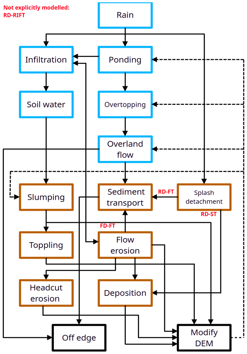
Figure 3 Flowchart of RillGrow. Blue-edged boxes indicate hydrological processes or stores, brown-edged boxes indicate erosional processes, and black-edged boxes are model specific. The codes (RD-ST, FD-FT, etc.) describe erosional sub-processes; see Kinnell (2001). Plain black lines represent process linkages, and dashed black lines represent feedback.

The model uses a time step for each iteration which is dynamically controlled by the maximum speed of cell-to-cell runoff during the previous time step to ensure that cell-to-cell flow in the model obeys the Courant et al. (1928) condition. With cell sizes of millimetres to centimetres, time steps are of the order of hundredths of a second. Thus, RillGrow simulations require considerable computing power for large grid sizes: simulations are, therefore (with current versions of the model), confined to plot-sized areas.

2.4 Input parameters and model runs

To perform the erosion modelling with a range of model input parameters, a Monte-Carlo-like approach was used. This employed Latin hypercube (LHC) sampling to draw the parameters approximately randomly. The parameter space was divided into bins, with sizes defined by the chosen parameter value range and the number of drawings. This LHC approach aims to ensure a near-random distributed sampling of parameter combinations so that the whole parameter space is covered and the variability of the data is represented. LHC sampling has been used to calibrate hydrological models (e.g. Singh et al., 2024).

Seven RillGrow input parameters were considered in this way:

• DEM base level, which is the vertical distance between the lowest DEM cell elevation and the plot outlet level;

• N for splash efficiency, which determines soil redistribution due to splash, i.e. RD-ST (raindrop detachment − splash transport) and RD-FT (raindrop detachment − flow transport) in Kinnell (2001);

• maximum flow speed, which is a cut-off for cell-to-cell runoff speed which cannot be exceeded;

• K for detachment, which determines soil detachability by flow, i.e. FD-FT (flow detachment − flow transport) in Kinnell (2001);

• radius of soil shear stress, which controls the size of the patch over which shear stress is distributed, which controls slumping (gravitational cell-to-cell movement of saturated cells which both exceed a given cell-to-cell gradient and which exceed a shear stress threshold);

• threshold shear stress for slumping; and

• angle of rest for slumped soil.

Whilst other input parameters could have been chosen, we focused on these following a first simple Monte Carlo simulation using 3000 runs and testing 12 parameters.

Subsequently, 2000 and 2400 RillGrow simulation runs were conducted for the laboratory and the field site, respectively, at the high-performance computing (HPC) centre of the Dresden University of Technology. As it was not practically feasible to save model outputs at every time step, selected points in time were chosen, with a higher temporal resolution at the beginning of the simulation and decreasing temporal steps later on. For the field site, in total, 36 temporal points (minutes 0.2, 0.5, 1, 2, 3, 5, and 7 and, afterwards, every 3 min until 90 min) were considered. For the laboratory site, 19 temporal points (minutes 0.1, 0.2, 0.5, 1, 2, 3, and 4 and then every 2.5 min until 30 min) were considered.

2.5 Objective functions for erosion model evaluation

Erosion model results were compared with measured sediment yield and measured DoDs, considering, in total, 10 different objective functions and their combinations. The objective functions for different observations were tested with regard to their suitability for calibrating the erosion model. We distinguish between three different spatio-temporal characteristics – i.e. space–time averaged, time averaged, and area averaged (Table 1) – and different options to calculate comparison metrics – i.e. total change, root mean squared error (RMSE), dynamic time warping (DTW) distance, and normalized Nash–Sutcliffe efficiency (NNSE). Also, observations from different sources, namely image-based elevation change (EC) models and sediment yield (SY) measurements, were used (Table 2). Finally, the combination of different objective functions was investigated.

Table 2 Summary of objective functions and their combinations used for the soil erosion model calibration.

2.5.1 Space–time-averaged data

This considers the total change in the measurements, for example, the change in the total sediment lost during the rainfall simulation experiment compared to the modelled sediment lost. Space–time-averaged EC refers to the cumulative height change measured at the end of the experiments (i.e. the difference, as in M3C2-PM, between the initial- and the final-time-slice DEM) compared to the modelled EC.

2.5.2 Time-averaged data

Here, we compare the observed and modelled spatial pattern of erosion. This involved two objective functions. The first objective function estimated the pixel-wise difference, i.e. a direct comparison of the measured 3D model and the simulated soil surface. To do this, the observed DEM must be resampled to the same resolution as the simulated raster. Calculated pixel height differences are eventually aggregated to an average value. The second objective function is a dense vector representation (DVR) using a deep learning (DL) method to calculate image embeddings, i.e. an abstract image representation summarized in one vector, to compare them in the latent (i.e. abstract) feature space. This approach is used here to assess the similarity in terms of spatial patterns. The DL approach is less sensitive to offsets in the position of rills (i.e. several-pixel differences in the position of the modelled rill compared with the observed rill). The CLIP (Contrastive Language–Image Pre-training; Radford et al., 2021) model was used to transform the images into the feature space because it has been shown to be robust across domains: this is especially relevant for our application with height images, which are usually not part of the training datasets. Afterwards, the cosine similarity score is used to derive a value of similarity between the transformed images. To perform this comparison, the DEMs were transformed into an 8-bit three-channel image prior to some filtering of strong height outliers to avoid artefacts by keeping only 95 % of the height values, with the remaining 5 % (i.e. the largest heights) being replaced by the closest inlier value. The best-performing model runs were chosen with regard to the average difference and similarity values of the final model run of each time series; i.e. we did not compare every simulated and observed 3D surface of a series but rather compared only the last ones.

2.5.3 Area-averaged data

Here, the comparison is between the time series of spatially averaged (i.e. whole-plot) changes. In the case of the EC data, the DoDs based on the M3C2-PM approach were used to estimate the average height change per point in time, thereby always considering the first DEM of the time series as the reference model for the change calculation of the subsequent models. The simulated DEMs were also differentiated using the first model as the reference to eventually receive the simulated time series of the modelled EC. To compare the time series, three different metrics were considered.

• RMSE is an accuracy metric that calculates the square root of the quadratic mean of the differences between the modelled and measured values.

• DTW distance is a measure that tries to find the optimal match between two sequences and whose remaining mismatch can be considered to be an estimate of the time series similarity. It has the advantage that it is invariant in relation to some non-linear behaviour. This metric has been applied to align complex time series of topographic change (Anders et al., 2021).

• NNSE is the preferred metric to assess model performance (Batista et al., 2019). It is a measure that relates the modelled error variance to the measured one. The closer the value to unity, the better the model predicts the erosion.

Thus, in total, six metrics were estimated, i.e. the three summarizing time series values calculated for both EC and SY comparisons.

2.5.4 Combinations of objective functions

Combinations of different objective functions were also evaluated. The multiple objective function approach considers eight different combinations (Table 2). For the multiple objective function approach, the best models were found by keeping the models whose metrics were within the top values; e.g. for finding the 10 best models, the objective function values were iteratively sorted and evaluated until at least 10 models remained within the top values of each list. We assume that the use of more objective functions enables us to deal better with equifinality (Beven, 2006) due to different processes being captured with different calibration metrics, although only two data sources were used as input, i.e. images and sediment yield measurements. For instance, the time-averaged spatial similarity compares the overall appearance of the rill network, whereas the RMSE of the time series of elevation change ideally captures overall erosion within the plot.

For the field experiment, results from the model runs often showed very strong artefacts. Therefore, a filter approach was applied that assumed smoother changes in the soil surface, including rill incision, to automatically detect and correspondingly exclude these faulty simulation runs. Elevation changes between the first and last DEM (i.e. the DoD) of each simulation run were smoothed using a Gaussian filter with a five-pixel kernel. The smoothed model was then subtracted from the original DoD to identify very strong changes. The approach is adopted from Onnen et al. (2020). If the difference is below an arbitrary threshold of 5 cm, the change in that pixel is considered to be valid. Finally, the ratio between the number of affected and non-affected artefact pixels is calculated, and if the ratio is below 0.2 % then the simulations are considered not to be plausible.

3 Results

Results are shown separately for the field and laboratory experiments. Animations of elevation changes in the soil surfaces of the field and laboratory rainfall simulation experiments may be viewed with Animations S1 and S2 in the Supplement for the field and laboratory, respectively. Note that some flickering is observable in both time series. This is due to the unavoidable circumstance of capturing images during rainfall, although rainfall does not fall continuously, leading to a slight increase in data noise. Nevertheless, image matching and DEM calculation were still possible because most drops were detected as outliers during the SfM processing.

3.1 Results from the field experiment

During the 90 min of the field rainfall simulation, with an intensity of 140 mm h⁻¹, 173.5 kg of sediment was lost from the plot. Total discharge was about 3100 L. Total net height changes measured for the entire plot (including the RoI) amounted to 1.2 cm. At the beginning of the rainfall experiment, a rill began to form in the bottom left of the plot. Rill growth then stopped. Later, a second rill began to form in the bottom centre of the plot and then began to cut backwards (i.e. upstream). Growth of this rill slowed after some time. Later, the left rill began to grow again, and this time it continued to cut backwards until the end of the experiment. The formation of wide head cuts was also observed during the experiment; these appear to be more like terraces and are present across the slope. They retreated upslope slightly but did not evolve into rills.

Large artefacts developed in many model simulations (Fig. 4). These artefacts show very large differences in terms of accumulation and erosion between directly neighbouring pixels, which is not a plausible erosion pattern. However, some objective functions of the time series still indicated a good fit between modelled and observed data, e.g. when considering the lowest values for DTW EC (7.8 cm) and SY (99 kg).

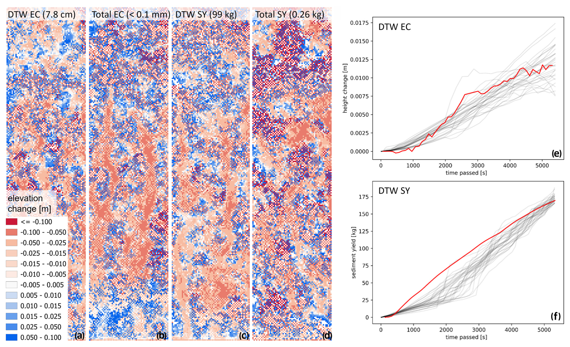
Figure 4 Although metrics of objective functions – e.g. time series of DTW of measured (red line) and simulated (grey lines) elevation change (EC) and sediment yield (SY) for the field simulation (f) – indicate good model fit, large artefacts in the final simulated model are visible (a–b). For the legend, see Fig. 2.

Also, the plotted time series of the 30 best simulated model runs, according to the objective function DTW, seemed to indicate a good capturing of the averaged EC by the erosion model. An exception was the best model runs found by the DTW SY, in which simulated splash was strongly underestimated (Fig. 4). However, total EC (0.1 mm) and SY (0.26 kg) differences show very good model run fits once again. Still, an inspection of the maps of the final DoDs shows that the best model run when applying only the EC-based metrics (Fig. 4, two left plots), i.e. without considering spatial patterns, leads to noisy model runs. This might be due to high positive and negative changes in immediate proximity, which are then cancelled during the averaging of the EC. If only SY-based metrics are used then not even rill patterns are visible in the best-simulated model runs (Fig. 4, two right plots). The good fits in the unfiltered simulation data were therefore found for the wrong reasons, i.e. due to the very strong artefacts, and so they do not reflect a good fit of parameters to describe the simulated erosion process.

Using our chosen objective functions alone did not provide sufficient information to automatically assess the plausibility of model outputs and, thus, the best input parameters. Only the additional assumption of smooth DEM changes enabled the removal of these implausible models. When the filter was applied, 279 model runs remained from the original 2000. Different relationships between the objective functions became clear after filtering (scatterplots in Fig. 5) and before filtering (Fig. S3). In the subsequent assessment of the field results, we considered only the filtered data.

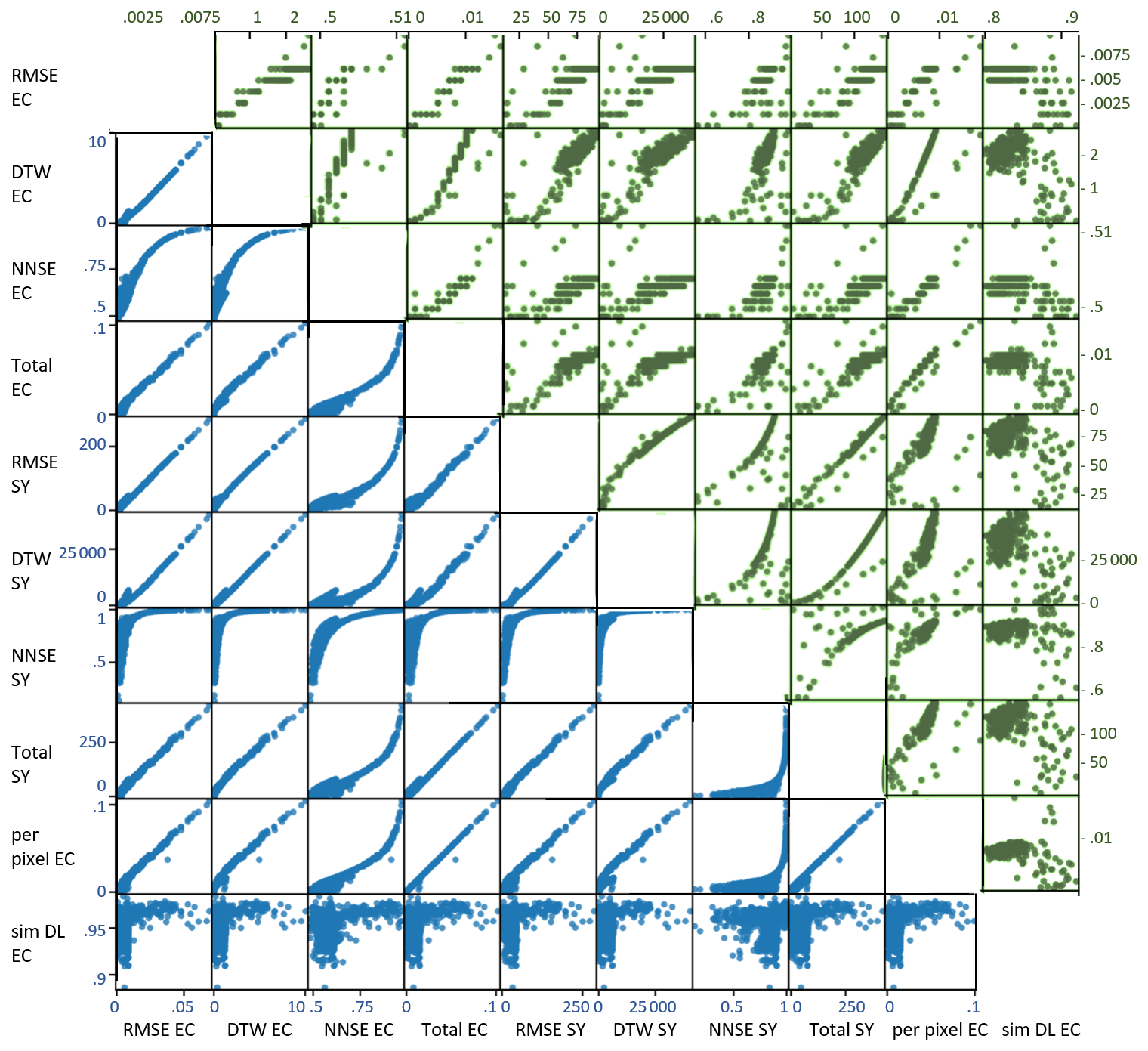
Figure 5 Scatterplots of values of objective functions for the field plot (EC in m – except for sim DL, which has no unit – and SY in kg). Blue scatterplots (lower triangle) correspond to the laboratory experiment, and green scatterplots (upper triangle) correspond to the field experiment. The objective functions and their abbreviations are explained in Table 2.

The relationship between the different metrics of the objective functions is not linear, except for that between RMSE and DTW EC, which indicates that the metrics capture different aspects of soil surface change due to erosion (Fig. 5). For example, the model run that has the lowest difference in terms of EC between simulated and observed data does not have to be the same model run with the lowest SY difference. The differences between the EC and SY metrics are more complex compared to the differences between those with the same data sources, i.e. camera-based or plot-outlet-measured. Nevertheless, in general, there is a dependence that is visible between the different metrics. This was favourable because we were looking to explore the behavioural parameter space constrained by different sources of data and objective functions. The assumption here is that the more diverse the objective functions are, the better the different aspects of the model will be captured. The objective functions that were chosen for the time series of EC (RMSE, DTW, and NNSE for EC) and total change (EC) fit well, which is also the case for the corresponding SY metrics. The DL-based similarity values reveal the most complex and least obvious relationship with the values of the other functions.

Next, we show the differences between the best model runs chosen according to the different objective functions which considered total changes (space–time-averaged), time series (area-averaged), and spatial patterns (time-averaged). Figure 6 depicts the final DoD of the best model runs, given the individual objective functions, as well as their combinations. All variants of the objective functions result in a best model run that appears to be realistic and that predicts at least three dominant rills, though with different lengths, widths, and depths. The predicted rills all reach quite far, compared with observations, into the belt of no erosion towards the upper end of the plot; also, only two main rills were observed. However, the observations for model evaluation were only considered for the RoI, within which the rills did, indeed, cross the whole length.

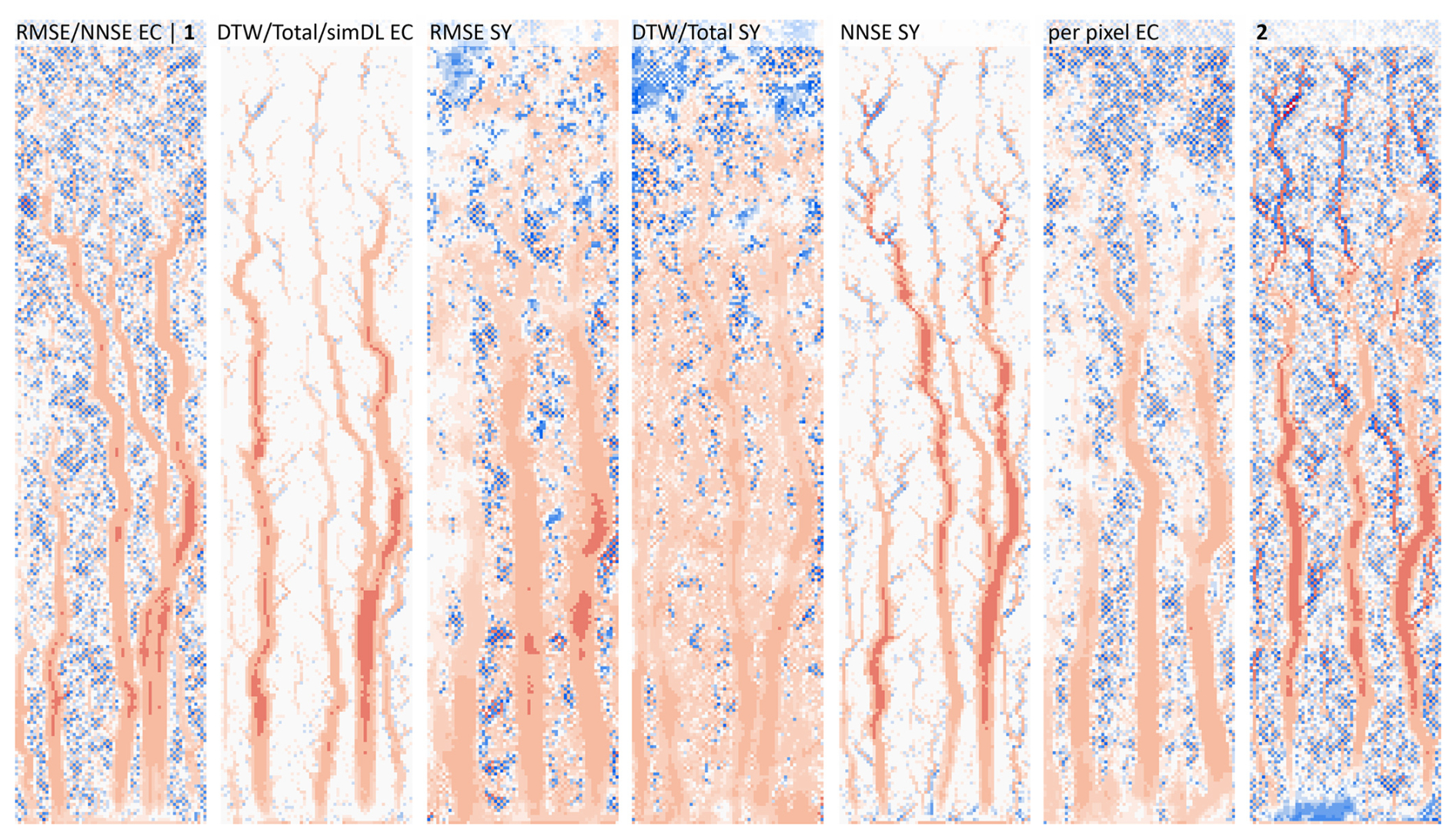
Figure 6 Simulated height change for single and combinations of objective functions (1: EC t_series, EC t_series and total, EC t_series and total and sp_pattern (no DL), EC t_series and total and sp_pattern; 2: SY t_series, SY t_series and total, EC and SY t_series, EC and SY t_series and total, EC and SY t_series and total and sp_pattern (no DL), all). For the legend, see Fig. 2. The objective functions and their abbreviations are explained in Table 2.

The best model runs differ when either single EC- or SY-based objective functions are used for evaluation. If combinations are considered, there is a difference between using only EC-based metrics and SY-based metrics or combinations of EC- and SY-based metrics. The same best model run resulted for DTW EC, total EC, and sim DL EC. Thus, EC metrics that consider space–time-averaged (total), area-averaged (DTW), or time-averaged (sim DL) characteristics all select the same model run. Further, in that model run, no artefacts are present. This is also the case for NNSE SY. The predicted SY for the best EC-metric-based model run is, however, about 30 kg (∼ 17 %) off from the measured total SY, but the predicted and measured total EC are almost identical. In the case of predicted total EC, the best NNSE-SY-based model run is off by 1 mm total EC and by about 24 kg total SY. However, the best model run that was found based on height changes also predicts a more pronounced left rill across almost the whole plot length, which is not the case for the best model run based on the NNSE SY metric. This indicates a potentially better performance of EC-based metrics in finding the best-fitting rill pattern. The best model runs for DTW, total, and sim DL EC and NNSE SY do not predict splash or inter-rill erosion, which does not fit the actual observation of strong splash effects (Fig. 6). More splash is modelled for a realization with better DTW and SY metrics. However, in that model run, the rill depth is too small. The widest rills are found for the best model run based on RMSE SY and per-pixel EC.

When considering the combination of objective functions, only two best model runs eventually remained. For all objective functions that consider only EC as a parameter (and the various combinations, i.e. EC t_series, EC t_series and total, EC t_series and total and sp_pattern (no DL), EC t_series and total and sp_pattern), only one model run remained. The second model run was indicated for all other objective function combinations that consider both EC and SY (i.e. SY t_series, SY t_series and total, EC and SY t_series, EC and SY t_series and total, EC and SY t_series and total and sp_pattern (no DL), all). Nonetheless, it is obvious that these two model runs still contain artefacts; also, they do not seem to model splash adequately. This might, however, be masked by the artefacts. Both model runs predict three main rills, which are deeper for the second model run, i.e. when EC and SY are considered for model evaluation. Time series from the erosion model runs (i.e. the area-averaged metrics) reveal a good fit by the 30 best model runs at the beginning of the simulation, when changes to the soil surface are still small (Fig. 7).

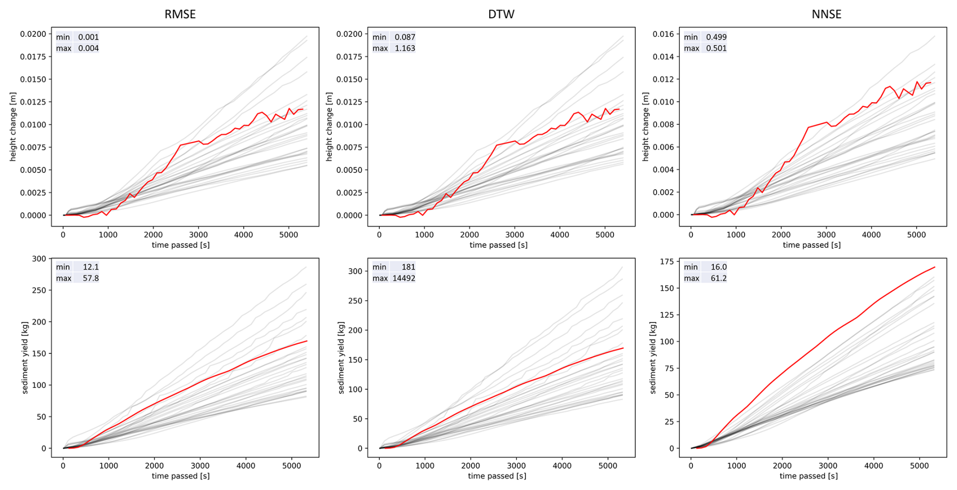
Figure 7 Time series of elevation change measured with time-lapse SfM and of sediment yield measured for the plot outlet of the 30 best models according to the objective functions of RMSE, DTW, and NNSE for the field plot. Note that the scales of the y axes differ. The objective functions and their abbreviations are explained in Table 2.

After about 30 min, the model runs begin to deviate strongly from the observations, independently of the considered objective function (RMSE, DTW, or NNSE) for EC. We noted that the erosion model runs were not able to capture the observed change in erosion rates: after a slow increase in erosion, after about 15 min, the erosion rate increased steeply then decelerated to a lower rate after about 40 min, which then remained nearly constant until the end of the experiment. However, the simulation runs depict more continuous erosion rates. Differences between modelled and simulated time series of SY are not as strong. A better fit with regard to the erosion rate and its change during the experiment is visible. Still, the erosion model runs tend to either overestimate or underestimate erosion throughout the experiment. Very few model runs fitted observations very closely. When considering NNSE, no model run fitted, and all the best model runs indicated underestimation.

Considering the observations alone, i.e. EC and SY, the temporal behaviour indicates a difference in both measures. The EC depicts stronger changes in erosion rate during the rainfall simulation compared to the SY rate, which is more stable. This difference might be due to the level of detection (LoD) of the photogrammetry-based data. Thus, only when changes exceed some threshold are they considered, potentially underestimating splash processes in the early rainfall phase.

The time series of the change in the spatial patterns (per-pixel EC and sim DL EC) also indicate, at the beginning, a small difference between simulations and observations since the changes in the soil surface early on in the experiment are still low. Later on, after about 15 min, the patterns become less similar. Figure 8 shows the similarity in terms of the spatial pattern for the top 30 model runs according to the averaged per-pixel EC and sim DL EC metrics. The DL-based approach further reveals that the stronger the changes are, the closer the similarity values again become; however, this is not the case for the per-pixel EC metric. This may indicate that it becomes easier to assess the similarity with DL as the spatial patterns become stronger due to increasing dominance of erosion rills, whereas, during the intermediate phase, the elevations of soil surfaces might be ambiguous due to greater noise.

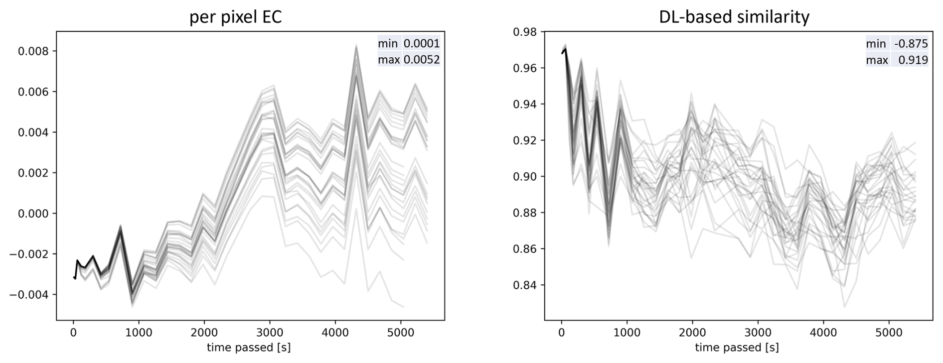
Figure 8 Time series of spatial-pattern metrics for 30 best models according to per-pixel EC and DL-based EC similarity metric for the field experiment. The objective functions and their abbreviations are explained in Table 2.

We assessed the 10 best model runs considering the different objective function options to evaluate the spread of the model input parameters. Figure 9 shows the parameters within the total para8meter range for the 10 best model runs according to the multiple objective function approach using all objective functions. It is clear that the parameters do not cluster tightly: equifinality is apparent here, with different combinations of model input parameters giving similarly good model fits according to the difference between observations and predictions as described by the different calibration metrics. The spread of parameter values through the whole parameter space remains, mostly for the single objective functions, as well as for their combinations. However, a closer look at the 10 best results for all objective functions solely indicates decreased ranges of the parameters determining soil detachability by flow and the threshold for shear stress for slumping because, in their combination with the other parameters, they no longer cover the whole of the parameter space but rather only cover partial areas; e.g. in the case of maximum flow velocity, there is an inverse correlation with soil detachability by flow. In general, very low flow detachment parameters were not considered, which highlights the preference for model runs with a stronger influence of flow detachment with transport by flow. Filtering of the artefacts from model runs is also visible in the parameter space because the larger splash efficiency values are mostly removed (i.e. in the upper range, only very few parameter values remained), indicating that raindrop detachment with transport by raindrop splash is not adequately described by the erosion model since the simulated influence of splash is not confirmed by the observations (i.e. DoDs).

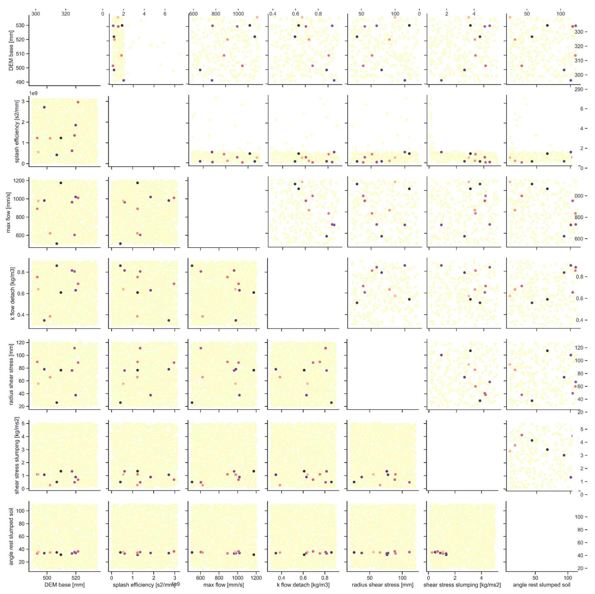
Figure 9 Parameter values of 10 best models considering all objective functions – lower triangle corresponds to the laboratory experiment, and upper triangle corresponds to the field experiment. The colours help to identify points belonging to the same model run.

Assessing the relationship between the model parameters and the metrics of the objective functions (Figs. S4–S10 in the Supplement) shows that the choice of lower values for the input parameter of “angle of rest for slumped soil” leads to better model performance, whereas larger values have no influence on the performance; i.e. no large changes with regard to the metrics can be seen, either because they remain high for the time series metrics or because they remain at a nearly constant value for the area- and space–time-averaged metrics. With regard to the parameter choices for DEM base level, radius of shear stress, and splash efficiency, no influence on model performance is visible when looking at the different metrics. Furthermore, it appears to be the case that, with larger choices for the values of the model input parameters for flow detachment and maximum flow velocity, a slightly better performance in terms of the model runs is given when considering the SY-based metrics. However, this relationship is not as clear for the EC-based metrics. Higher shear stress slumping threshold values lead to better erosion model performances when considering EC metrics, but the performance worsens if SY metrics are considered.

None of the model runs did a good job of predicting the observed rill pattern from the field experiment. Neither the number of rills (two) nor their locations were adequately modelled. However, some of the model runs did predict the rill on the left side of the plot and the rill in the middle of the plot. Nevertheless, no model run indicated that the rill on the left would become more dominant later during the rainfall simulation and that the rill in the middle would be dominant in the beginning of the experiment and then would stop growing.

3.2 Results from the laboratory experiment

During the 30 min rainfall simulation in the laboratory, a total of 80.8 kg of sediment was lost from the plot, and the corresponding discharge was about 395 L. The total net height change measured for the plot was 1.6 cm. Thus, although the rainfall simulation intensity was the same as that of the field experiment, a larger negative height change (about 25 %) was seen, as well as greater sediment yield (considering the fact that, for the laboratory plot, nearly half of the SY had already been lost after only one-third of the total experiment duration for the field plot). Discharge amounted to only about 8 % of the field runoff. These differences are mainly due to the significantly higher slope gradient for the laboratory experiment. The animation (Fig. S1) of elevation changes during the field experiment shows the formation of a rill network which is markedly different from the network developed during the field experiments. At first, a dominant rill formed on the lower-right side of the plot. A second main rill then developed in the lower third of the plot, on the left side. After about 15 min, the left rill merged with a third rill that began to grow at the bottom of the plot after about 10 min, cutting upslope until it met the other rill. At the end of the experiment, an intricate dendritic rill pattern was observable, especially in the upper third of the plot, which was also dominated by sheet erosion, draining into the two main rills. The rill network formed in the first 15 to 20 min and then changed little, mainly just deepening.

Again, in contrast, to the field experiment, in the laboratory rainfall simulation, no strong artefacts were observed in the erosion model output. Therefore, no filtering was necessary, and all 2400 model runs could be used for the evaluation using the different single objective functions (Fig. 10). Although the best model runs of the various calibration functions predict the observed filigree rill pattern and/or a few single strong rills, none of them adequately represent the strong sheet erosion. In the best model runs based on the area-averaged parameters (RMSE, DTW, NNSE), four dominant rills that are wide and deep and situated across the whole plot region are predicted. Considering total SY for calibration yields three obvious rills, with the right-hand rill fitting the observed data well as it is also bifurcated. However, none of the SY-based best model runs capture the overall fine rill pattern. The best model runs for the space–time- and area-averaged EC-based metrics also predict wide rills covering the lower region of the plot, which is closer to the camera-based observations. The observed total SY is underestimated by 12 kg (DTW, RMSE, total EC) to 16 kg (NNSE EC), whereas the residual of the predicted total SY for the best SY-based model runs ranges between 1 kg (DTW SY) and 3 kg (NNSE, RMSE SY). The best model run for the objective function considering per-pixel EC is the only one that predicts two dominant rills. However, these rills are still too wide and short compared with observations. The best model run for the second metric focusing on the spatial pattern, i.e. sim DL EC, predicts the formation of many small rills. Thus, it is closest to the observed dendritic rill pattern, but the rills are too shallow, and this model run completely misses the observed sheet erosion.

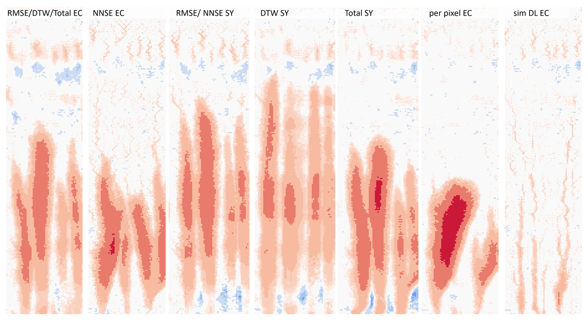
Figure 10 Simulated height change of the best model with regard to the single objective functions. For the legend, see Fig. 2. The objective functions and their abbreviations are explained in Table 2.

When combining the objective functions, it is not possible to find a single best model run that fits the observations well (Fig. 11). In the case of parameters based on EC and SY time series, model runs predict patterns with rills that are too wide and too long and which cover the whole plot. The combination of objective functions considering only EC-based metrics, including the spatial pattern, indicates model runs with rill erosion dominating in the lower to the middle parts of the plot; however, these are still too long, and there is a belt of no erosion in the upper region of the plot. If SY-based metrics are combined with EC-based ones then predicted rills are shorter but still do not resemble the observations as the rills remain too wide. Overall, in the camera-based observations in the upper region of the plot, strong sheet erosion is visible, which is not predicted by the erosion model.

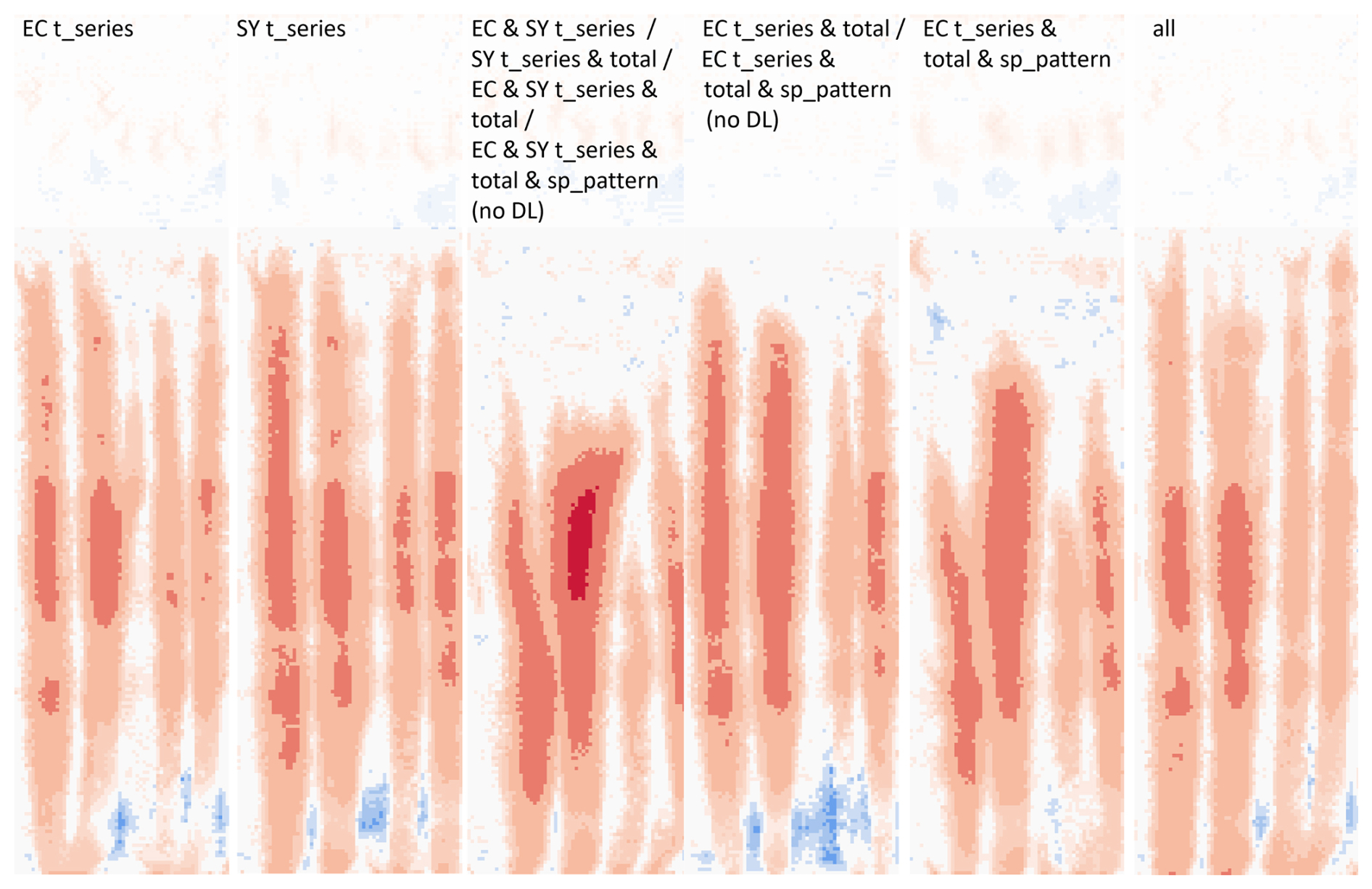
Figure 11 Simulated height change of the best model with regard to the multiple objective functions. For the legend, see Fig. 2. The objective functions and their abbreviations are explained in Table 2.

Relationships between the different calibration metrics are more obvious for the laboratory experiment (Fig. 5). Correlations between all objective function values, except for NNSE and the DL-based spatial-pattern comparison, are clearly linear. The relationship between the values of the NNSE SY and EC and the remaining metrics is obvious and non-linear. The DL-based similarity metric alone reveals an unclear relationship with the values of the other functions.

When assessing the temporal behaviour of the 30 best model runs according to the area-averaged metrics, the EC-based approaches reveal model runs that fit well or tend to underestimate soil erosion in the middle period of the experiment (Fig. 12). The best model runs according to the RMSE and NNSE EC do a better job of predicting height change over time, while the DTW-EC-based models give a best fit at the beginning and end of the experiment (as is expected due to the way in which the DTW is calculated). The NNSE-EC-based simulations show the largest variance between the 30 best model runs at the end of the experiment. In contrast to the field experiment, the rates of change for the observed EC and SY are similar in the laboratory rainfall simulation, which may result from more intense change at the beginning of the experiment, leading to crossing of the LoD threshold early on. The best model runs according to the SY-based calibration values also fit the observations well. The RMSE- and NNSE-SY-based best model runs overestimate erosion, especially at the beginning but also slightly throughout the rainfall experiment. The NNSE-based best model runs scatter strongly towards the end of the experiment. The best model runs according to the DTW SY metric reveal a stronger variation with regard to the temporal behaviour of the sediment yield, with a few model runs strongly underestimating erosion.

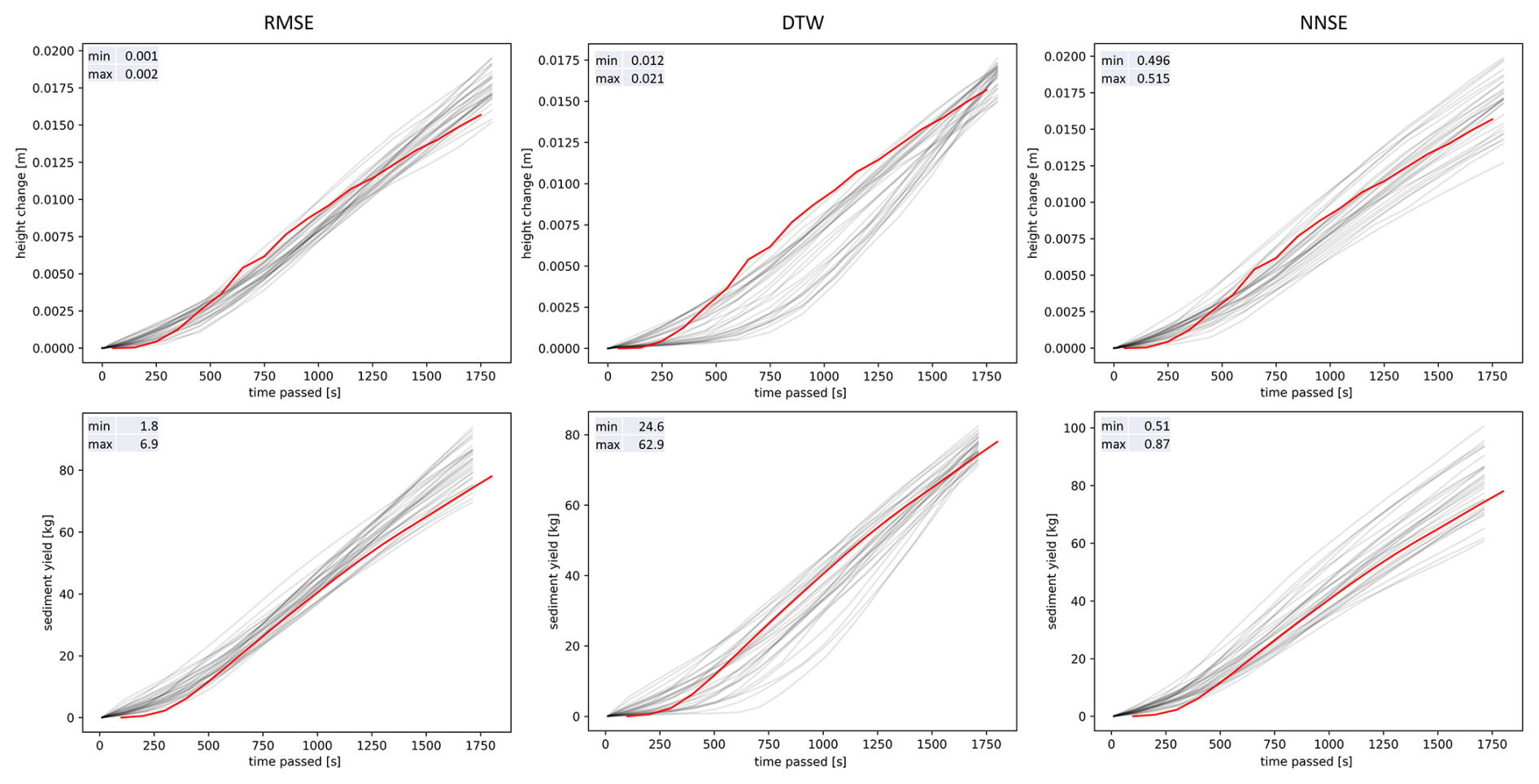
Figure 12 Time series of elevation change measured with time-lapse SfM and of sediment yield measured for plot outlet of the 30 best models according to the objective functions of RMSE, DTW, and NNSE for the laboratory plot. Note that the scales of the y axes differ. The objective functions and their abbreviations are explained in Table 2.

In both the field and the laboratory experiments, the spatial-pattern metrics indicate a high agreement between model results and reality at the beginning of the experiment. Later in the experiments, these begin to diverge when considering the per-pixel EC (Fig. 13). However, the best model runs according to the DL-based metric already show an increase in the deviation between observations and the model very early on in the experiment; towards the end, the differences decrease again. This is not surprising because the 30 best model runs were chosen using the difference of the last model runs in the time series. In general, model runs of the laboratory experiment were more similar to each other than was the case for model runs of the field experiment.

Figure 13 Time series of spatial-pattern metrics for 30 best models according to per-pixel EC and DL-based EC similarity metric for the laboratory experiment. The objective functions and their abbreviations are explained in Table 2.

Compared to the field experiment, the combination of objective functions enables a more obvious narrowing down of the range of parameter values with regard to the input parameters of the threshold of shear stress for slumping and the angle of rest for slumped soil, both of which are in favour of lower values (Fig. 9). For the input parameter of distance to the DEM base level, lower values are chosen for the 10 best model runs. The remaining parameters are spread across the entire range. For the laboratory experiment, relationships between the erosion model input parameters and the metrics of the objective functions indicate similar characteristics compared to the field experiment, except for the SY and when considering the parameter of the threshold of shear stress for slumping (Figs. S11–S17). Overall, no model run did a good job of predicting the response of the soil in the laboratory rainfall simulation experiment to the multiple and interacting processes of soil erosion. Rills were too long and wide, and no finely detailed rill pattern was predicted.

4 Discussion

This evaluation of a single soil erosion model used three approaches for spatio-temporal averaging (Table 1). While other erosion model evaluations (e.g. Favis-Mortlock et al., 1996; Jetten et al., 1999) have considered multiple erosion models, few if any previous erosion model evaluations have considered all three spatio-temporal averaging approaches. An important finding from this study is that each averaging approach, as exemplified by each group of objective functions, illuminates different aspects of erosion model performance, as discussed below. No single objective function is capable of identifying all of the strengths and weaknesses of the model tested. Thus, as we appreciate more strongly the interacting temporal and spatial complexities of soil erosion – whether at the process-dominated plot scale, as in this study, or the connectivity-controlled catchment scale (Favis-Mortlock et al., 2022) – and incorporate representations of this complexity into future erosion models, it is clear that we will need approaches to model evaluation of the kind described in this study.

A particular challenge when comparing measured and modelled patterns of rill erosion results from the problem of small spatial offsets in rill location. A modelled rill network might, as judged by eye, be very similar to an observed rill network. But a simple pixel-by-pixel comparison of measured and modelled DEMs could still give poor results since rills may well be spatially offset between the two DEMs, perhaps by very small distances. Additionally, measured and modelled rill depths may differ. There is much less of a problem when considering inter-rill changes since these are dispersed across the whole of the eroding area, and, thus, averaged values can be used. AI-based similarity objective functions (Radford et al., 2021), as used in this study, could provide a potential solution to this issue. Such objective functions can give a clear measure of the fit between models and observations even if the rills are not at identical locations.

We found that the best field experiment model runs using either EC-based single objective functions, i.e. DTW, total, and sim DL, which suggests that, in some cases, an ensemble of objective functions might not be needed. However, it also became clear that there is a sensitivity towards the choice of the single objectives because, for the metrics of RMSE, NNSE, and per-pixel EC, another best model run was found. Finding the best model runs using only EC-based measures suggests that the erosion model calibration might be possible without using sediment yield observations in certain scenarios. This has important implications for the usage of our approach to also calibrate models at larger scales, i.e. when time series of catchment data via UAV or aerial measurements may not be available.

The calibration metric DTW is not the most suitable for the SY-based measurements in the field experiment. However, if it is EC-based, the best model run was found to outperform the fit of the RMSE- and NNSE-EC-based metrics. This may be due to the averaging of the SY changes with no spatial consideration, whereas the averaged EC values are still based on spatial measurements. The best temporal behaviours of soil surface change (EC) or SY were captured before the artefact filtering; i.e. the DTW, RMSE, and NNSE values and corresponding plotted time series indicated a very good model fit. It is clear that splash redistribution is, indeed, an important process in our two experiments. However, the erosion model was not able to represent this process adequately. Further work is needed to avoid creating the artefacts that make the model outcome implausible.

When using time-lapse SfM photogrammetry to measure soil erosion, it must be considered that erosion-masking processes, such as soil compaction and settling, can lead to faulty erosion measurements (Kaiser et al., 2018; Epple et al., 2025). In these two experiments, such processes are assumed to be negligible due to the application of very strong rainfall events on relatively compacted soils (soil bulk density of 1.23 t m⁻³). Similar considerations apply when using laser scanners, e.g. Wang and Lai (2018).

From the perspective of future work, this study has clearly indicated weaknesses in some process representations within RillGrow, particularly splash redistribution. Work to improve this is ongoing. In addition, the computational needs of the model meant that the multiple model runs required by the current study used a great deal of computing power and time. A parallel-processing version of RillGrow is being developed.

In addition to considering changes in DEM elevation, it might also be useful in future studies to consider measurements of ponding and runoff forming at the soil surface (Zamboni et al., 2025) or spatially distributed velocity quantities (Wolff et al., 2024). These can be used to provide further calibration and/or evaluation opportunities focusing on the hydrological rather the sedimentological processes.

Another approach for future work could focus on the assessment of weighting the different objective functions. This is of interest because this study reveals that some objective functions are more important than others, such as when considering spatial patterns versus time series of averaged change metrics (e.g. DTW EC versus sim DL EC and their combinations, i.e. EC t_series and total and sp_pattern in the field experiment). We tested a weighted error after standardizing the objective function values. However, such a uniform approach did not produce good results for the field experiment; i.e. the best model runs contained only very small rills. Thus, the optimum weighting of the different functions is not known. Another potential improvement is the consideration of the parameter distribution. The 10 or 30 best model runs revealed that the output is not one set of parameters but actually a set of parameter distributions. However, these distributions are not independent; i.e. if one parameter is chosen, this means that a specific other needs to be drawn. Therefore, in the future, conditional drawings should be considered (i.e. Bayes' principle).

5 Conclusions

This study advances the calibration and evaluation of soil erosion models by considering various objective functions that consider spatio-temporal aspects differently. Several thousand runs of the erosion model RillGrow were performed with parameters drawn approximately randomly by means of a Latin hypercube approach. Outputs from these model runs were compared to sediment yields measured during field- and laboratory-based rainfall simulation experiments, and model outputs were compared to SfM-photogrammetry-derived observations, i.e. representations of soil surface change with spatial resolutions of a few centimetres and temporal resolutions of 10 s. Ten calibration metrics were used to find the best-performing model runs.

Results highlight the need for more sophisticated evaluation techniques that go beyond traditional space–time averaging methods. Different spatio-temporal averaging approaches illuminate different aspects of model performance, indicating that no single objective function could fully capture the complexities of erosion processes. The study also identified challenges in model evaluation, such as the issue of spatial offsets in rill locations, and suggests AI-based similarity functions as a potential solution. Additionally, the study clearly identified limitations in the process representations in the version of RillGrow used in the study, particularly with regard to splash erosion. Such a finding is very useful for prioritizing ongoing refinement of the erosion model.

The exploration of alternative calibration metrics and the potential for parallel processing to address computational demands illustrate the evolving landscape of erosion modelling. Our findings suggest that future research should focus on refining objective functions that also consider novel observations of the soil erosion processes, as such observations are likely under future global change. Future research should also consider parameter distributions to improve calibration outcomes.

Overall, this study strongly emphasizes the need for more nuanced evaluation of erosion models, including the incorporation of spatial-pattern comparison techniques. This is necessary to provide a deeper understanding of any erosion model's capabilities. Only with such improved model evaluations will we be able to adequately develop and evaluate a future generation of soil erosion models, which will be vital tools in forecasting and managing the erosional impacts of future global change.

Appendix A: List of abbreviations

CA	Cellular automaton
CLIP	Contrastive Language–Image Pre-training
DEM	Digital elevation model
DL	Deep learning
DoD	DEM of differences
DTW	Dynamic time warping
DVR	Dense vector representation
EC	Elevation change
FD-FT	Flow detachment − flow transport (Kinnell, 2001)
GCP	Ground control point
LHC	Latin hypercube
LoD	Level of detection
NNSE	Normalized Nash–Sutcliffe efficiency
PM	Precision map
RD-FT	Raindrop detachment − flow transport (Kinnell, 2001)
RD-ST	Raindrop detachment − splash transport (Kinnell, 2001)
RMSE	Root mean square error
RoI	Region of interest
SfM	Structure from motion
SLR	Single-lens reflex
SY	Sediment yield
UAV	Unoccupied aerial vehicle