Insights into the prediction uncertainty of machine-learning-based digital soil mapping through a local attribution approach

Machine learning (ML) models have become key ingredients for digital soil mapping. To improve the interpretability of their predictions, diagnostic tools such as the widely used local attribution approach known as SHapley Additive exPlanations (SHAP) have been developed. However, the analysis of ML model predictions is only one part of the problem, and there is an interest in obtaining deeper insights into the drivers of the prediction uncertainty as well, i.e. explaining why an ML model is confident given the set of chosen covariate values in addition to why the ML model delivered some particular results. In this study, we show how to apply SHAP to local prediction uncertainty estimates for a case of urban soil pollution – namely, the presence of petroleum hydrocarbons in soil in Toulouse (France), which pose a health risk via vapour intrusion into buildings, direct soil ingestion, and groundwater contamination. Our results show that the drivers of the prediction best estimates are not necessarily the drivers of confidence in these predictions, and we identify those leading to a reduction in uncertainty. Our study suggests that decisions regarding data collection and covariate characterisation as well as communication of the results should be made accordingly.

1 Introduction

Maps of soil physical properties, such as cation exchange capacity, pH, soil organic content, and hydraulic properties; chemical properties, such as concentrations of heavy metals (arsenic, mercury, etc.) and radionuclides (caesium-137, plutonium-239+240); and target-oriented indicators, such as erodibility and soil compaction (see, for example, Panagos et al., 2022), are essential for multiple types of studies, such as pollution assessment, urban planning, and construction design. In recent years, these maps have led to many advances in improving spatial prediction in the domain of digital soil mapping, denoted by DSM (McBratney et al., 2003), with the development of methods and approaches based on either the geostatistical framework (Chilès and Desassis, 2018) or machine learning (denoted ML) techniques (Wadoux et al., 2020).

Beyond spatial prediction, the question of uncertainty in spatial prediction has emerged as a key challenge (Heuvelink and Webster, 2022, Sect. 4). Historically, this question has been addressed with kriging (see, for example, Veronesi and Schillaci, 2019, for a discussion for DSM). Techniques based on ML have been increasingly used or adapted for this purpose. For instance, the popular quantile random forest model (e.g. Vaysse and Lagacherie, 2017) has been used to produce soil information worldwide in the SoilGrids 2.0 database together with uncertain information (Poggio et al., 2021). Along these lines, improvements to validation procedures have been proposed (Schmidinger and Heuvelink, 2023) together with tools for assessing prediction error and transferability (Ludwig et al., 2023).

However, quantifying the uncertainty is only one part of the problem, and there is an interest in gaining deeper insights into the influence of each covariate on the overall prediction uncertainty. This is the objective of global sensitivity analysis (Saltelli et al., 2008), which can be conducted within two settings: either “factor fixing” to identify noninfluential covariates or “factor prioritisation” to rank the covariates in terms of importance. The expected results can be of different types: the former setting provides justification for simplifying the spatial predictive model by removing the noninfluential covariates, whereas the latter setting provides justification for prioritising future characterisation efforts by focusing on the most important variables. In DSM, this question has been addressed with the tools of variance-based global sensitivity analysis (i.e. the Sobol' indices, as implemented by Varella et al., 2010) or with variable importance scores together with potentially recursive feature elimination procedures (as implemented by Poggio et al., 2021, and Meyer et al., 2018). Both approaches provide a “global” answer to the problem of sensitivity analysis, i.e. by exploring the influence over the whole range of variation in the covariates. However, these methods do not enable us to measure the influence of the covariates locally, i.e. for a prediction at a certain spatial location.

Recently, an alternative local approach was proposed by relying on a popular method from the domain of interpretable machine learning (Molnar, 2022) based on Shapley values (Shapley, 1953). This method has shown promising results in attributing the contributions of each covariate to any spatial prediction (Padarian et al., 2020; Wadoux et al., 2023; Wadoux and Molnar, 2022).

To date, the application of Shapley values to DSM has focused mainly on the prediction best estimate, and little information has been provided on the local prediction uncertainty. Motivated by a case of pollution concentration mapping in the city of Toulouse, France (Belbeze et al., 2019), we aim to investigate how to use Shapley values to decompose the local uncertainty, measured by either an interquantile width or a variance estimate. Our objective is to explore the relationship between the drivers of the prediction best estimate and the drivers of confidence in the predictions. Providing evidence of differences in the dominant drivers is expected to have implications in terms of data collection and covariate characterisation. Communication of the results is also expected to be adapted accordingly. Figure 1 illustrates the type of result that can be derived with the approach. In this example (based on the synthetic test case fully detailed in Sect. 2.1), the mean prediction (best estimate, left panel) of the variable of interest at a certain location does not have the same contributors as the local uncertainty measured by the interquartile width (right panel). The group of covariates including the maximum and mean temperatures of the warmest quarter of the year (named T_mean-max) was identified as the first and second most important contributors, respectively. The identification of the least influential group of covariates also differed across both cases; this is illustrated by the mean diurnal range, T_range, which has little impact on the prediction result but strongly influences the confidence in the result.

Figure 1 Example of SHAP-based decomposition of the prediction best estimate (modelled by the conditional mean of a random forest model; panel a) and of the prediction uncertainty (modelled by the interquartile width estimated via a quantile random forest model; panel b) for the variable of interest in the synthetic test case (fully described in Sect. 2.1) at a certain location in the study area. Each horizontal bar represents the contribution to the prediction (indicated by the vertical dashed line) of the considered covariates (indicated on the vertical axis) that correspond to the mean diurnal range, T_range, to the group of covariates that includes the maximum and mean temperatures of the warmest quarter of the year, T_mean-max, and to the precipitation of the wettest month, P_wettest. Note the differences in the ordering of the groups, which indicates that the contributors to the mean and to the uncertainty estimate differ.

The remainder of the paper is organised as follows. We first describe two application cases that motivated this study. In Sect. 3, we provide further details on the statistical methods used to estimate the local contributions to the prediction uncertainty. In Sect. 4, we apply the methods and provide an in-depth analysis of the differences in the drivers of prediction best estimates and uncertainty. In Sect. 5, we discuss the practical implications of the proposed procedure and its transferability to global-scale projects.

2 Case study

2.1 Synthetic test case

The first test case is synthetic. It aims to predict a virtual species suitability surface, denoted by y, over central Europe (Fig. 2). This surface is calculated based on six bioclimatic covariates defined in Table 1 (with prior normalisation between 0 and 1), which were extracted from the WorldClim dataset (available at https://www.worldclim.org/data/bioclim.html, last access: 25 September 2024), as follows:

$$\begin{array}{}\text{(1)}& {\displaystyle }\begin{array}{rl}{\displaystyle }y\left(s\right)=& {\displaystyle }\mathrm{10}\times T_{\text{range}}\left(s\right)+\mathrm{5}\times T_{\text{max}}\left(s\right)+\mathrm{5}\times T_{\text{mean}}\left(s\right)\\ {\displaystyle }& {\displaystyle }+\mathrm{5}\times P_{\text{wettest}}\left(s\right)+{\mathrm{10}}^{-\mathrm{4}}\times P_{\text{driest}}\left(s\right)\\ {\displaystyle }& {\displaystyle }+{\mathrm{10}}^{-\mathrm{4}}\times P_{\text{coldest}}\left(s\right).\end{array}\end{array}$$

By construction, this model has the following two characteristics that are used here to validate the proposed methods described in Sect. 3.3: (1) the last two covariates have negligible influence and (2) the covariates T_max and T_mean are strongly dependent. The dataset is based on the vignette of the R package CAST, which is available at https://hannameyer.github.io/CAST/articles/cast02-AOA-tutorial.html (last access: 25 September 2024). A series of 25 “virtual” soil samples were randomly extracted (highlighted by square-like markers in Fig. 2) across the study area.

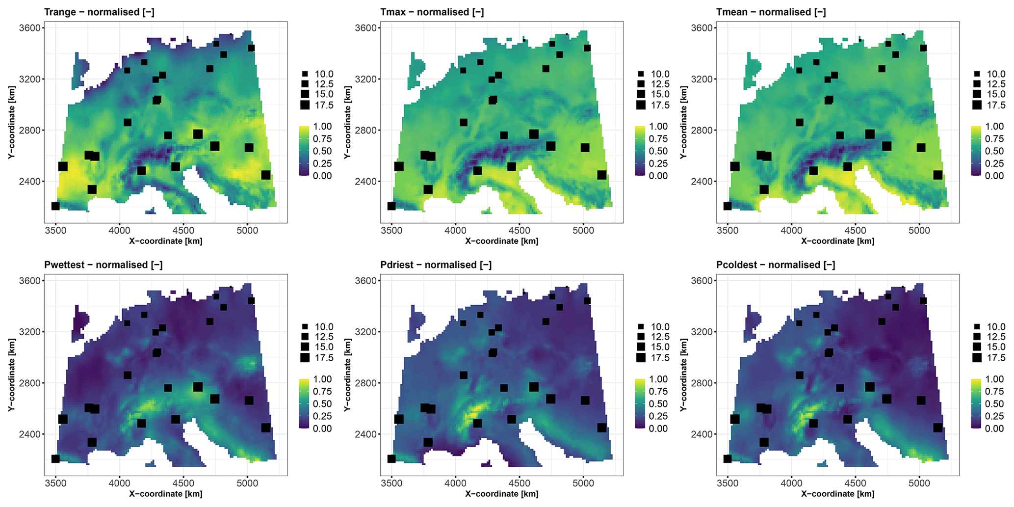
Figure 2 Covariates (with prior normalisation between 0 and 1) used in the synthetic test case (see Table 1 for a detailed description). The spatial distributions of the 25 soil samples are indicated by square-shaped markers. The size of each square is proportional to the synthetic variable calculated from the covariates based on Eq. (1).

Table 1 Description of the covariates for the synthetic test case.

2.2 Real test case

The real case focuses on DSM to predict the total petroleum hydrocarbon (C10–C40) concentration over the city of Toulouse (located in southwestern France) as part of the definition of urban soil geochemical backgrounds (see the comprehensive review by Belbeze et al., 2023). In this case, petroleum hydrocarbons have multiple sources, such as road and air traffic, industrial emissions, and residential heating. The presence of this pollutant may inhibit several soil functions and hence prevent the delivery of associated ecosystem services (Adhikari and Hartemink, 2016). A primary soil function that may be jeopardised is the ability of the soil to provide a platform for human activities in a risk-free environment. Petroleum hydrocarbons in soil pose a risk to human health via several pathways – namely, direct soil ingestion, which is a particularly sensitive pathway for young children; exposure through respiration via vapour intrusion into buildings; and contamination of groundwater used for drinking water purposes. Notably, our study uses the data of this case to illustrate and discuss the applicability of the proposed approach and is not meant to supplement the results of Belbeze et al. (2019).

We use 1043 soil samples collected over a depth interval [0,2] m to analyse the logarithm (base 10) of the C10–C40 hydrocarbon concentration expressed in milligrams per kilogram (Fig. 3). We aim to predict the concentration over the whole city of Toulouse using a fine grid of spatial locations (one point every 100 m, i.e. >45 000 grid points) with the covariates described in Table 2. Figures 4 and 5 depict the spatial distributions of the considered covariates of continuous and categorical types, respectively.

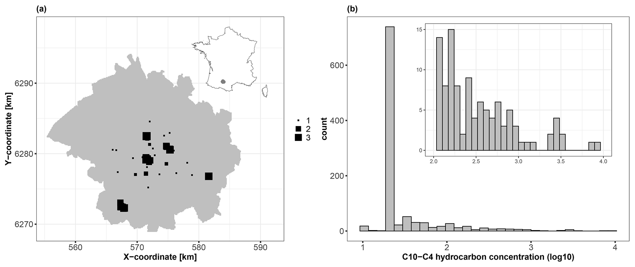
Figure 3 (a) Spatial locations of the 1043 soil samples (square-like markers) across the city of Toulouse, which is located in southwestern France (see the location in the top-right inset map). The size of each square is proportional to the logarithm (base 10) of the C10–C40 hydrocarbon concentration (expressed in mg kg⁻¹). (b) Histogram of the logarithm (base 10) of the C10–C40 hydrocarbon concentration (expressed in mg kg⁻¹), with a magnified view of the interval 2.0–4.0 (top-right inset panel).

Table 2 Description of the covariates of the real test case.

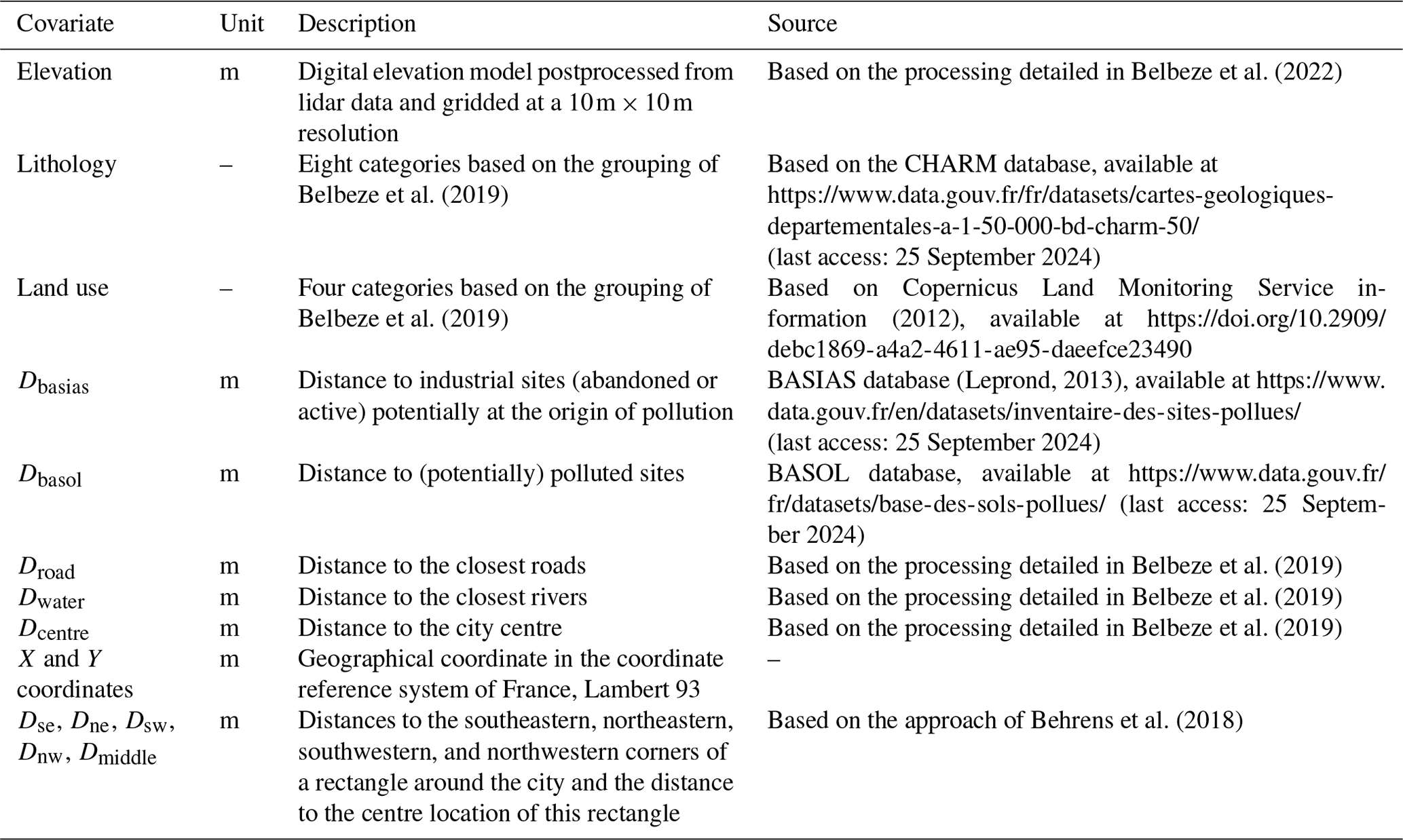
In addition to these covariates, we follow the approach proposed by Behrens et al. (2018) to better account for spatial dependence: we also consider seven additional covariates – namely, the two geographical coordinates, X and Y, and five geographical covariates that correspond to the distances to the southeastern, northeastern, southwestern, and northwestern corners of a rectangle around the city (denoted by D_se, D_ne, D_sw, and D_nw) and the distance to the centre location of this rectangle (denoted by D_middle). A total of 15 covariates are considered.

3 Methods

3.1 Local attribution framework

We first consider that the value of the variable of interest y(s) (e.g. a soil property or pollutant concentration) at a given spatial location s is related to d covariates, $\mathbf{x}\left(s\right)=\mathit{\left\{}{x}_{\mathrm{1}}\right(s),x_{\mathrm{2}}(s),\mathrm{\dots },x_d(s\left)\mathit{\right\}}$. The mathematical relationship is modelled by an ML model (denoted by f(.)), where f(x(s)) is assumed to resemble y(s) as closely as possible; that is, y(s)≈f(x(s)). The ML model also provides a measure of the uncertainty (denoted by u(s)) of this prediction that is related to x(s) through the function g(.), which may differ from f(.). In this study, we focus on the random forest model (denoted by RF) used for regression (Breiman, 2001) and on its quantile regression variant, denoted by qRF (Meinshausen, 2006) because this ML model has proven to be very efficient in multiple studies of DSM, as outlined in the introduction. Further details are provided in Appendix B. To reflect the magnitude of the RF prediction uncertainty u(s) at spatial location s, we use the interquantile half-width (denoted by IQW_α) at a given level α, defined as follows:

$$\begin{array}{}\text{(2)}& {\displaystyle }\begin{array}{rl}{\displaystyle }u\left(s\right)& {\displaystyle }=g\left(\mathbf{x}\right(s\left)\right)={\text{IQW}}_{\mathit{\alpha }}\\ {\displaystyle }& {\displaystyle }=q^{\frac{\mathrm{1}+\mathit{\alpha }}{\mathrm{2}}}\left(y\right|\mathbf{x}\left(s\right))-q^{\frac{\mathrm{1}-\mathit{\alpha }}{\mathrm{2}}}(y\left|\mathbf{x}\right(s\left)\right),\end{array}\end{array}$$

where q^τ(y|x(s)) is the conditional quantile at level τ. In particular, the interquartile width corresponds to IQW_α=0.50.

Our objective is to decompose u(s) at a given spatial location s as a sum of the ${\mathit{\mu }}_{i=\mathrm{1},..,d}\left(s\right)$ specific to the values of the covariates x(s) within the setting of the additive “feature attribution approach” (as defined by Lundberg and Lee, 2017, Sect. 2) as follows:

$$\begin{array}{}\text{(3)}& u\left(s\right)=g\left(\mathbf{x}\right(s\left)\right)={\mathit{\mu }}_{\mathrm{0}}+{\sum }_{j=\mathrm{1}}^p{\mathit{\mu }}_j\left(s\right),\end{array}$$

where μ₀ (named the base value) is a constant value (see the definition in Sect. 3.2). This decomposition can also be applied to f(.) as described in previous studies, as indicated in the introduction.

Importantly, Eq. (3) does not aim to linearise g(.) but to compute the contribution of each covariate to the particular prediction uncertainty value g(x(s)). This means that the decomposition provides insights into the influence of the particular instance of the covariates x(s) relative to g(x(s)): (1) the absolute value of μ(s) informs on the magnitude of the influence at location s directly expressed in physical units, which facilitates interpretation, and (2) the sign of μ(s) indicates the direction of the contribution, i.e. whether the considered covariate influences the prediction upwards or downwards in relation to the base value, μ₀. Both aspects are outlined in Fig. 1; the width of the horizontal bar and the arrow are indicators of (1) and (2), respectively. To quantify μ(s) in Eq. (3), we rely on the SHapley Additive exPlanations (SHAP) approach, which was developed by Lundberg and Lee (2017) based on the Shapley values described in Sect. 3.2.

Figure 4 Covariates of continuous type over the city of Toulouse (see Table 2 for a detailed description).

Figure 5 Covariates of categorical type over the city of Toulouse. (a) Lithology (MT: medium terrace alluviums, LT: low terrace alluviums, LP: low plain alluviums, MB: major riverbed alluviums, MO: molasses, and FI: fill materials). (b) Land use (AGR: agriculture, FOR: forests and grasslands, and IND: industrial and commercial economic activities); see Table 2 for a detailed description.

3.2 Shapley additive explanations

The SHAP approach relies on the Shapley value (Shapley, 1953), which is used in game theory to evaluate the “fair share” of a player in a cooperative game; i.e. it is used to fairly distribute the total gains between multiple players working cooperatively. It is a “fair” distribution in the sense that it is the only distribution that satisfies some desirable properties (efficiency, symmetry, linearity, and “dummy player”). See the proofs by Shapley (1953) and Aas et al. (2021, Appendix A) for a comprehensive interpretation of these properties from an ML model perspective.

Formally, we consider a cooperative game with d players and let $D_S\subseteq D=\mathit{\{}\mathrm{1},\mathrm{\dots },d\mathit{\}}$ be a subset of $\left|D_S\right|$ players. We define a real-valued function that maps a subset D_S to its corresponding value, $\text{val}:{\mathrm{2}}^{D_S}\to \mathbb{R}$, and measures the total expected sum of the payoffs that the members of D_S can obtain by cooperation. The gain that the ith player obtains is defined by the Shapley value with respect to val(.):

$$\begin{array}{}\text{(4)}& {\displaystyle }\begin{array}{rl}{\displaystyle }\mathit{\mu }& {}_i\left(s\right)=\\ {\displaystyle }& {\displaystyle \frac{\mathrm{1}}{d}}{\sum }_{D_S\subseteq D\backslash \mathit{\left\{}i\mathit{\right\}}}{\left(\begin{array}{c}d-\mathrm{1}\\ \left|D_S\right|\end{array}\right)}^{-\mathrm{1}}(\text{val}\left(D_S\cup \left\{i\right\}\right)-\text{val}(D_S\left)\right).\end{array}\end{array}$$

Equation (4) can be interpreted as the weighted mean over the contribution function differences for all subsets D_S of players not containing player i. This approach can be translated for ML-based prediction by viewing each covariate as a player and by defining the value function val(.) as the expected output of the ML model conditional on ${\mathbf{x}}_S^{\ast }$, i.e. when we only know the values of the subset D_S of inputs (Lundberg and Lee, 2017). This approach is flexible with respect to the output of the ML model and can be applied to the conditional mean of the RF model and to the uncertainty measure computed with the qRF model (Eq. 2).

Formally, the following applies:

$$\begin{array}{}\text{(5)}& \text{val}\left(D_S\right)=\mathrm{E}\left(h\left(\mathbf{x}\right)|{\mathbf{x}}_{D_S}={\mathbf{x}}_{D_S}^{\ast }\right),\end{array}$$

where h(.) can correspond to either the conditional mean, denoted by f(.), or the uncertainty estimate, denoted by g(.), and E(.) is the expectation operator.

In this setting, the Shapley value can then be interpreted as the contribution of the considered covariate to the difference between the prediction, h(x^∗), and the base value, μ₀. The latter can be defined as the value that would be predicted if we did not know any covariates (Lundberg and Lee, 2017). In the application case, we are interested in pollution prediction; in this context, we choose μ₀=0, which means that if we do not know any covariates, no pollution is expected (and there is no uncertainty). In this way, μ_i in Eq. (3) corresponds to the change in the expected model prediction if f(.) is used (or in the uncertainty if g(.) is used) when conditioning on that covariate and explains how to depart from 0. By construction, μ_i=0 indicates the absence of influence for the ith covariate related to the dummy player property of the method. In addition, the sum of the inputs' contributions is guaranteed to be exactly $h\left({\mathbf{x}}^{\ast }\right(s\left)\right)-{\mathit{\mu }}_{\mathrm{0}}$, which is related to the efficiency property of the method.

In this study, we aim to calculate the Shapley values for both the prediction best estimates modelled by f(.) and the uncertainty modelled by g(.). To facilitate comparison across the study area between these different prediction objectives, we use a scaled version of the Shapley absolute value, i.e. $\mathit{\mu }\left(s\right)/\left(f\right({\mathbf{x}}^{\ast }\left(s\right)\left)\right)$, expressed in percentages. This means that the contributions, regardless of the prediction objective, are analysed in Sect. 4 with a common scale, which is chosen here as the value of the prediction best estimate for the given considered instance.

In practice, the computation of the Shapley value may be demanding because Eq. (4) implies covering all subsets D_S (the number of which grows exponentially with the number of covariates, d, i.e. as 2^d) and Eq. (5) requires solving integrals of dimension 1 to d−1. When the SHAP approach is applied to a large number of spatial locations (in our case, >45 000), the computational complexity is high. To alleviate the computational burden, a possible option is to rely on the group-based approach proposed by Jullum et al. (2021), which can be used to adapt Eq. (4) for a group of covariates. Considering a partition $\mathbf{G}=\mathit{\{}{G}_{\mathrm{1}},G_{\mathrm{2}},\mathrm{\dots },G_g\mathit{\}}$ of the covariate set D, the Shapley value for the ith group of covariates, G_i, is as follows:

$$\begin{array}{}\text{(6)}& {\displaystyle }\begin{array}{rl}{\displaystyle }\mathit{\mu }& {}_{G_i}\left(s\right)=\\ {\displaystyle }& {\displaystyle \frac{\mathrm{1}}{g}}{\sum }_{T\subseteq \mathbf{G}\backslash \mathit{\left\{}{G}_i\mathit{\right\}}}{\left(\begin{array}{c}g-\mathrm{1}\\ |T{|}_g\end{array}\right)}^{-\mathrm{1}}\left(\text{val}\right(T\cup \mathit{\left\{}{G}_i\mathit{\right\}})-\text{val}(T\left)\right),\end{array}\end{array}$$

where the summation index T runs over the groups in the sets of groups G\G_i and $|T{|}_g$ is the number of groups in T. This means that this group Shapley value is the game-theoretic Shapley value framework applied to groups of covariates instead of individual covariates. The group Shapley values possess all the Shapley value properties. The practical advantage of working with groups is that computing Eq. (6) has a relative computational cost reduction of 2^d−g, hence making possible the use of an exact method by considering all combinations of covariates for computing the Shapley values.

This definition raises the practical question of how to define groups. As explained by Jullum et al. (2021), this definition can be based on knowledge/expertise, i.e. on information that makes sense in relation to the problem at hand. The main advantage is that this facilitates the interpretation of the Shapley values. The second grouping option, which is complementary to the one based on expertise, consists of identifying covariates that provide redundant information because they share a strong dependency. The groups of dependent covariates can be identified with a clustering algorithm (see Hastie et al., 2009, Chap. 14) by taking the matrix of pairwise similarities as input. This approach does not, however, ensure that the effect of dependence among the covariates is completely removed, which may influence the SHAP results, as was extensively investigated by Aas et al. (2021). To account for this, we rely on the method proposed by Redelmeier et al. (2020) using conditional inference trees (Hothorn et al., 2006) to model the dependence structure of the covariates.

3.3 Overall procedure

The proposed approach, named group-based SHAP (see the implementation details in Appendix A), comprises three steps.

Step 1 aims to build and train the RF models based on the dataset of soil samples together with the covariate values, which is named the training dataset. The RF hyperparameters correspond to the number of variables at which to possibly split in each node (denoted by m_try) and the minimal node size at which to split (denoted by n_s). Their values are tuned via a repeated 10-fold cross-validation process (Hastie et al., 2009, Chap. 7). Although the RF model is efficient in taking into account many covariates, performing a screening analysis prior to the SHAP application within the cross-validation procedure is useful for facilitating its implementation. By reducing the number of covariates directly during the construction of the RF, the SHAP computational burden can be largely alleviated, as discussed in Sect. 3.2, and the applicability to global-scale projects where hundreds of covariates are present can be improved (see the discussion in Sect. 5.2).

To eliminate the covariates of negligible influence, different options are available in the literature (see, for example, the procedure based on recursive feature elimination described by Poggio et al., 2021). Here, we propose relying on a popular method in the ML community – namely, the dependence measure based on the Hilbert–Schmidt independence criterion (HSIC) of Gretton et al. (2005). This generic measure has the advantages of being applicable (1) to any type of dependence, i.e. linear, monotonic, or nonlinear (see the discussion by Song et al., 2022); (2) to mixed variables, i.e. continuous or categorical (as in our case, described in Sect. 2); and (3) without the use of RF importance measures, for which limitations have been identified in the literature, as has been extensively discussed (see, for example, Bénard et al., 2022, and references therein). In addition, the combination of HSIC with a hypothesis testing procedure (El Amri and Marrel, 2024) provides a rigorous setting for quantifying the significance of the considered covariate through the computation of p values. Further details are provided in Appendix C.

Step 2 is optional and aims to identify groups of covariates. The objective is twofold. First, by grouping covariates suitably with respect to the problem at hand, the Shapley values can be easily interpreted. This can be done based on expert knowledge or/and by identifying covariates that share a strong dependence to reduce the redundancy of information, for instance, using the HSIC pairwise dependence measure (Appendix C). The second practical implication is a reduction in the computational burden of the Shapley value estimation, as discussed in Sect. 3.2.

Step 3 is to compute the Shapley values associated with each covariate or group identified in Step 2 to decompose the prediction uncertainty provided by the qRF model (trained in Step 1).

4 Results

4.1 Application to the synthetic test case

Using the 25 randomly selected soil samples described in Sect. 2.1, we construct an RF model to estimate the conditional mean, which is used as the best estimate of the prediction, and a qRF model to estimate the interquartile width (IQW), which is used as the uncertainty estimate. To select the RF parameters ns and m_try, we repeat a 10-fold cross-validation exercise 25 times (Hastie et al., 2009, Chap. 7) by varying ns from 5 to 10 and m_try from 1 to 4. The number of random trees is fixed to 1000; preliminary tests have shown that this parameter has little influence provided that it is large enough. This tuning procedure selects the pairs ns, m_try for which the average relative absolute error is minimised, identifying ns=5 and m_try=3 as the combination that results in the lowest error of 6.8 % (averaged over 25 replicates of the 10-fold cross-validation) with a frequency of 72 % (i.e. 18 replicates out of 25). A screening analysis is performed within the cross-validation procedure using HSIC measures combined with a hypothesis testing procedure using the sequential random-permutation-based algorithm developed by El Amri and Marrel (2022) with up to 5000 random replicates. Averaged over the replicates of the 10-fold cross validation (repeated 25 times), the p values for the first four covariates reach a maximum value of 2 % (Sect. S1 in the Supplement). The p values of the last two covariates are 16 % (with a standard deviation of 10 %) and 20 % (with a standard deviation of 12 %). Using a significance threshold of 5 %, this means that the last two covariates are not statistically significant; hence, the number of covariates can reasonably be reduced from six to four. This result is consistent with the construction of the synthetic case described by Eq. (1).

Using the trained RF model, Fig. 6 shows the best estimate of the true value of the synthetic variable of interest (panel a) and the prediction best estimate (panel b) together with the uncertainty measure (panel c) at 10 000 grid points across the European study area (with a spatial resolution of $\approx \mathrm{13.5}\mathrm{km}\times \mathrm{13.5}\mathrm{km}$). The RF predictions reproduce the true spatial distribution relatively well (comparing panels a and b in Fig. 6), with an average relative absolute error of approximately 5 %. The uncertainty indicator reaches the highest values (highlighted in yellow in Fig. 6c) where observations are sparsely distributed, particularly in the Alps (zone Z₁) and in northern Germany (zone Z₂). It is important to note that our objective here goes beyond improving the predictive capability of the RF model: given this level of prediction uncertainty (Fig. 6c), we aim, in the following, to investigate the main drivers of this uncertainty and whether they differ from the drivers of the best estimate of the prediction (Fig. 6b).

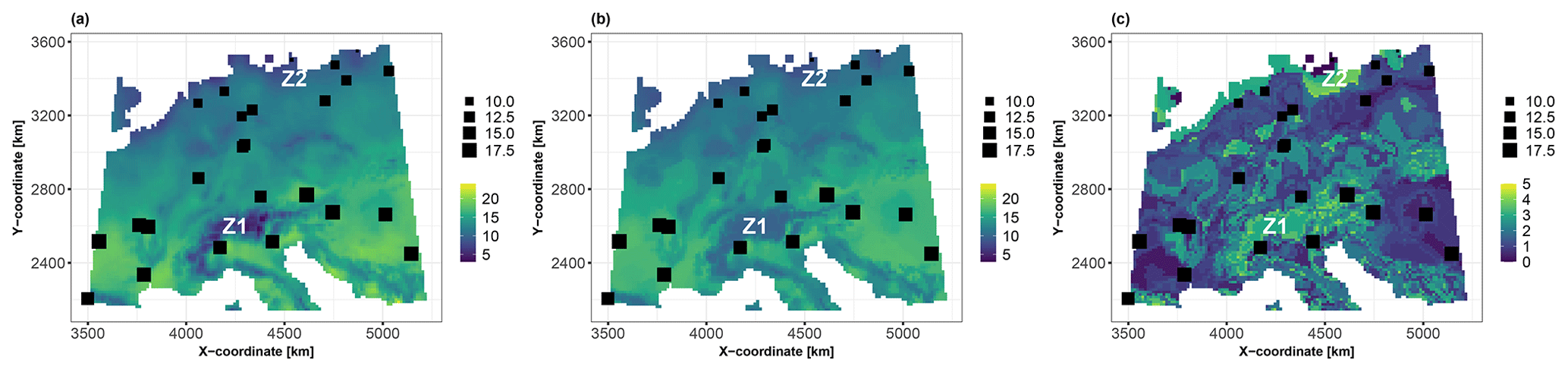
Figure 6 (a) Spatial distribution of the synthetic variable of interest modelled by Eq. (1). (b) Prediction best estimate using the conditional mean of the RF model. (c) Interquartile width (IQW) computed using the 25th and 75th percentiles of the qRF model. The 25 soil samples are indicated by squares whose sizes are proportional to the value of the synthetic variable of interest. The results are more specifically discussed in Sect. 4.1 for the zones indicated by Z₁ and Z₂.

To ease the interpretation, we group the temperature variables T_max and T_mean because they are, by nature, physically related. To further support this choice, we apply a partitioning around medoids clustering algorithm (Rdusseeun and Kaufman, 1987) using the matrix of the pairwise HSIC dependence measures (provided in Sect. S1). The average silhouette width reaches 0.32 and 0.41 for two and three groups, respectively, which justifies the use of three groups – namely, T_mean-max, T_range, and P_wettest.

Using the trained RF model and the selected groups of covariates, we apply the group-based SHAP approach to decompose the data at the 10 000 grid points of the study area. An example of this analysis at the grid point of coordinates 4206729 m, 2149423 m is provided in Fig. 1. To facilitate comparison across the study area, we plot the scaled Shapley values, as defined in Sect. 3.2, and use them to map the contributions to the prediction best estimate (i.e. the conditional mean; Fig. 7a) and to the corresponding uncertainty (i.e. IQW; Fig. 7b). With regard to the prediction best estimate, the upper panels of Fig. 7 show that the three groups of covariates have Shapley values in the range [25,50] % over ≈75 % of the whole study area. Figure 7 shows that the major contributors to the prediction best estimate and to the uncertainty differ. This is exemplified by the two zones where the uncertainty is the highest (see Fig. 6c). In the central zone around the Alps (zone Z₁ in Fig. 7), the major contributors to the best estimate and to the uncertainty are P_wettest (with contributions in the range of 50 %–75 %), the group T_mean-max (with contributions in the range of 10 %–25 %), and T_range over a more limited spatial extent. On the other hand, in northern Germany (zone Z₂ in Fig. 7), P_wettest contributes the most to the uncertainty, with contributions in the range of 10 %–25 %, whereas the group T_mean-max contributes the most to the prediction mean, with contributions in the range of 50 %–75 %. These differences in importance may be related to the scarcity of soil samples in both zones (see Fig. 2). This means that the training data are not representative of both zones. The practical implication is that decisions regarding the characterisation of the covariates are different in these two zones; this is discussed in more detail in Sect. 5.1.

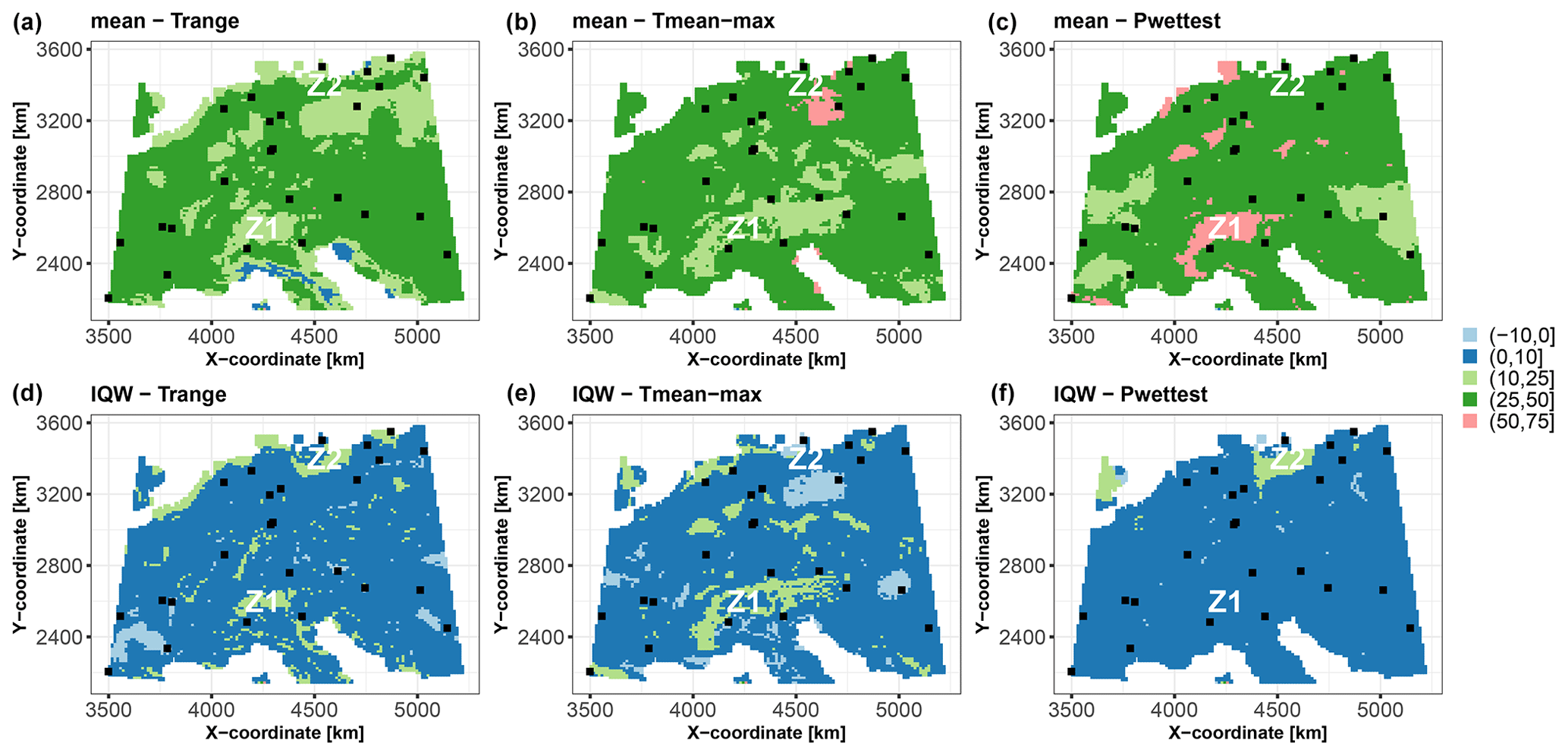
Figure 7 Scaled Shapley values (in %) for the synthetic test case considering the prediction best estimate modelled by the RF conditional mean (a–c) and the prediction uncertainty modelled by the qRF interquartile width (IQW; d–f). The black squares indicate the spatial locations of the 25 soil samples. The results are more specifically discussed in Sect. 4.1 for the zones indicated by Z₁ and Z₂.

4.2 Application to the real case

We construct an RF model using the 1043 soil samples described in Sect. 2.2. We use the conditional mean as the best estimate of the prediction and the interquartile width IQW as the uncertainty estimate, with the 25th and 75th percentiles computed using a qRF model. In our case, one additional difficulty is related to how the points are spatially distributed. Figure 3a shows that the points are spatially clustered as they overrepresent some regions while underrepresenting or even missing others. This situation might lead to biased predictions because the same weight is given to every point, and thus regions with high sampling density are overweighted. To alleviate this problem, we follow an approach similar to that of Bel et al. (2009). First, we use an inverse sampling intensity weighting to assign more weight to the observations in sparsely sampled zones and less weight to the observations in densely sampled zones. Second, to estimate the sampling intensity, we use a two-dimensional normal kernel density estimation with bandwidth values estimated based on the rule of thumb of Venables and Ripley (2002). Finally, the inverse sampling intensity weights, with prior normalisation to between 0 and 1, are used for RF training during bootstrap sampling (see Appendix B) to create individual trees with different probability weights by following a method similar to that of Xu et al. (2016).

To select the RF parameters ns and m_try, we use a cross-validation exercise similar to that used for the synthetic case. This tuning procedure selects the pairs of ns and m_try for which the average relative absolute error is minimised, yielding ns=5 and m_try=2 as the combination that results in the lowest error of ≈12 % (averaged over 25 replicates of the 10-fold cross-validation) with a frequency of 76 % (i.e. 19 replicates out of 25).

Figure 8 Screening analysis showing the p values (denoted pval) of the HSIC-based test of independence (described in Appendix C) for the Toulouse case. The dots indicate the mean values estimated over the replicates of a 10-fold cross-validation (repeated 25 times). The lower and upper bounds of the error bars are defined as ± 1 standard deviation. When the dot merges with the error bar, the value of the standard deviation is low. The vertical red line indicates the significance threshold at 5 %. When the p value is lower than 5 %, the null hypothesis should be rejected; i.e. the considered covariate has a significant influence on the hydrocarbon concentration and is retained in the RF construction.

A screening analysis is performed within the cross-validation procedure using HSIC measures combined with a hypothesis testing procedure. Figure 10 shows the statistics of the p values calculated over the replicates of the 10-fold cross-validation (repeated 25 times). Several observations can be made:

• The distance to potentially polluted sites, D_basos, has a minor influence, contrary to the distance to industrial sites, D_basias (abandoned or active). This is due to the high dependence of D_basos (whose HSIC is on the order of 0.93–0.95; Sect. S2 in the Supplement) on elevation and geographical coordinates. This is also supported by Fig. 3, which suggests that polluted sites tend to be located in relatively low-lying areas in the vicinity of the city centre. In other words, the inclusion of D_basos in the analysis is redundant with respect to the information provided by the covariates on which it is dependent.

• Land use has a strong impact, whereas lithology appears to have little impact, with a p value on the order of 25 %, i.e. larger than the significance threshold. This is interpreted as being related to the hydrocarbon nature of the pollution, which is less strongly related to geological processes than heavy-metal pollution, for instance.

• The distance to roads was not included even though its relation to hydrocarbon concentration was expected. This is less due to its dependence on the other covariates, whose HSIC values are as high as 0.14 (Sect. S2), than to its very dense spatial distribution: the value of this covariate varies very little over a large area, as indicated by the almost homogeneous colour in Fig. 3; i.e. very few zones are discriminated by this covariate in this case.

• Out of all the cross-validation replicates, nine covariates have a statistically significant influence on hydrocarbon concentration, considering a significance threshold of 5 %. These covariates are retained in the construction of the final RF model that is used for the application of the group-based SHAP approach.

Figure 9 shows the prediction (panel a) of the hydrocarbon concentration together with the uncertainty measurement (panel b) at the grid points across the city with a spatial resolution of 100 m×100 m. Notably, a large proportion of the city has a predicted concentration varying between 1 and 2 (on a log ₁₀ scale), with the exception of the southeastern part, where the concentration is predicted to be >3. In this zone, the uncertainty in the prediction is the highest, with values ranging up to ≈2.5. Outside this zone, a large proportion of the study area has uncertainty estimates of <1.0, with some zones having uncertainties of <0.01, particularly in the vicinity of the observations.

Figure 9 (a) Prediction best estimate of the hydrocarbon concentration (log ₁₀ scale) for the city of Toulouse using the conditional mean of the RF model. The soil samples are indicated by squares whose sizes are proportional to the log ₁₀ of the hydrocarbon concentration. (b) Interquartile width (IQW) computed using the 25th and 75th percentiles of the qRF model (expressed on the same scale as the hydrocarbon concentration).

To ease the interpretation of the Shapley values, we define two groups of covariates whose contributions are considered together with the land use and the elevation:

• The group D_basias-water includes D_basias and D_water. The analysis of the joint influence is meaningful because this group reflects the general tendency of industrial sites to be located close to a water supply.

• The geographical group includes D_ne, D_se, D_nw, D_sw, and the Y coordinate. This group of covariates was introduced to improve the predictive capability of the RF (see Sect. 2.2). Interpreting the respective influence of each of these individual covariates is often difficult in practice, and grouping them makes sense in this regard.

To support these choices, we analyse the pairwise dependence measure (Sect. S2), which confirms the moderate-to-high pairwise dependence of all variables in this group. This analysis also indicates that land use has a low dependence on the other variables.

Using the trained RF model, we apply the group-based SHAP approach to decompose the data at >45 000 grid points in the study area. As for the synthetic test case, we compute the scaled Shapley values and use them to map the contribution to the prediction best estimate (i.e. the conditional mean; Fig. 10, left) and to the corresponding uncertainty (i.e. IQW; Fig. 10, right). With regard to the prediction best estimate, the left panels of Fig. 10 show that the four covariate groups have contributions, to some extent, of approximately the same order of magnitude. The different groups have high influence, with scaled Shapley values within the range [25,50] % but in different areas of the city – namely, in the central part of the city for elevation and land use, i.e. in low-lying industrial areas (Fig. 4); in the western part for D_basias-water; and in the eastern part for the geographical group. The geographical group has the largest contribution in the southeastern part of the city where the predicted values are the largest, as outlined by the dark-green zone in Fig. 10, left. This is also confirmed by the analysis of the boxplots provided in Sect. S2. Regarding the prediction uncertainty, the scaled Shapley's values are mainly in the range [0,25] %, but with some particular areas where the determining factors for either the best prediction estimate or uncertainty or both are not necessarily the same.

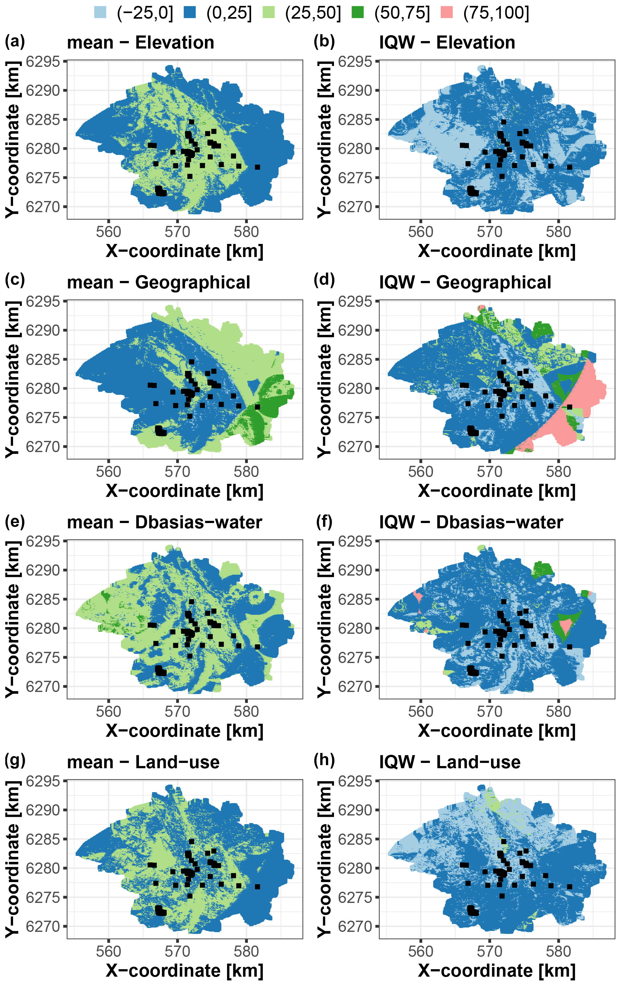
Figure 10 Scaled Shapley values (in %) for each group of covariates of the Toulouse test case considering the prediction best estimate using the RF conditional mean (a, c, e, g) and the prediction uncertainty using the qRF interquartile width (IQW) (b, d, f, h). The black squares indicate the locations of the soil samples used for RF training.

Three distinct situations are identified that are relevant from the viewpoint of uncertainty management. The first situation corresponds to the locations outlined in Fig. 11, where the groups of covariates significantly contribute to the prediction best estimate, with a scaled Shapley value exceeding that of the uncertainty by more than 25 %. Interestingly, the main contributors to this situation are the three groups that are relevant to the soil prediction problem as opposed to the geographical group, whose objective is to account for spatial dependence. This gives some confidence in the process underlying the RF prediction because it indicates that the best estimate is controlled mainly by the soil-relevant predictors. This also indicates that their influence on the prediction is not masked by the use of geographical covariates, i.e. the use of spatial surrogate covariates, also called pseudocovariates, as discussed by Wadoux et al. (2020, Sect. 3.3).

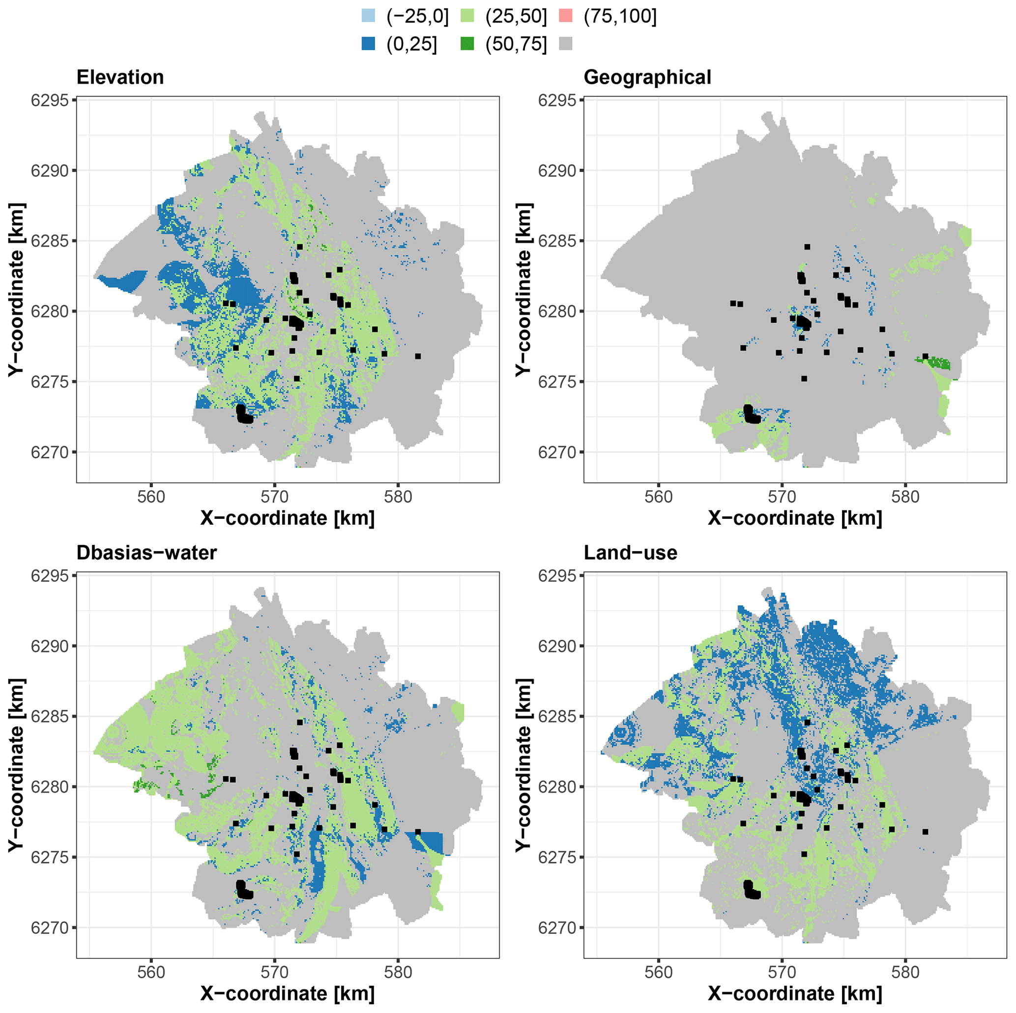
Figure 11 Locations where each corresponding group of covariates significantly contributes to the best estimate, with a scaled Shapley value exceeding that of the uncertainty by more than 25 %. The colours indicate the scaled Shapley value for the best estimate. The areas in grey correspond to grid points where the condition is not met. The black squares indicate the locations of the soil samples used for RF training.

An examination of the distribution of the corresponding covariates (Fig. 12) reveals that these locations have elevation values and distances D_basias and D_water of the same order of magnitude as those in the training dataset, resulting in an “optimal” prediction situation in which the RF model is used to predict cases that are relatively similar to those used for its training. In the areas where land use contributes most to this situation, we show (Fig. 12, bottom right-hand panel) that this is linked to agricultural areas and forests, i.e. areas where there is a lower chance of finding potentially polluted sites, as is also shown by the analysis of the training dataset.

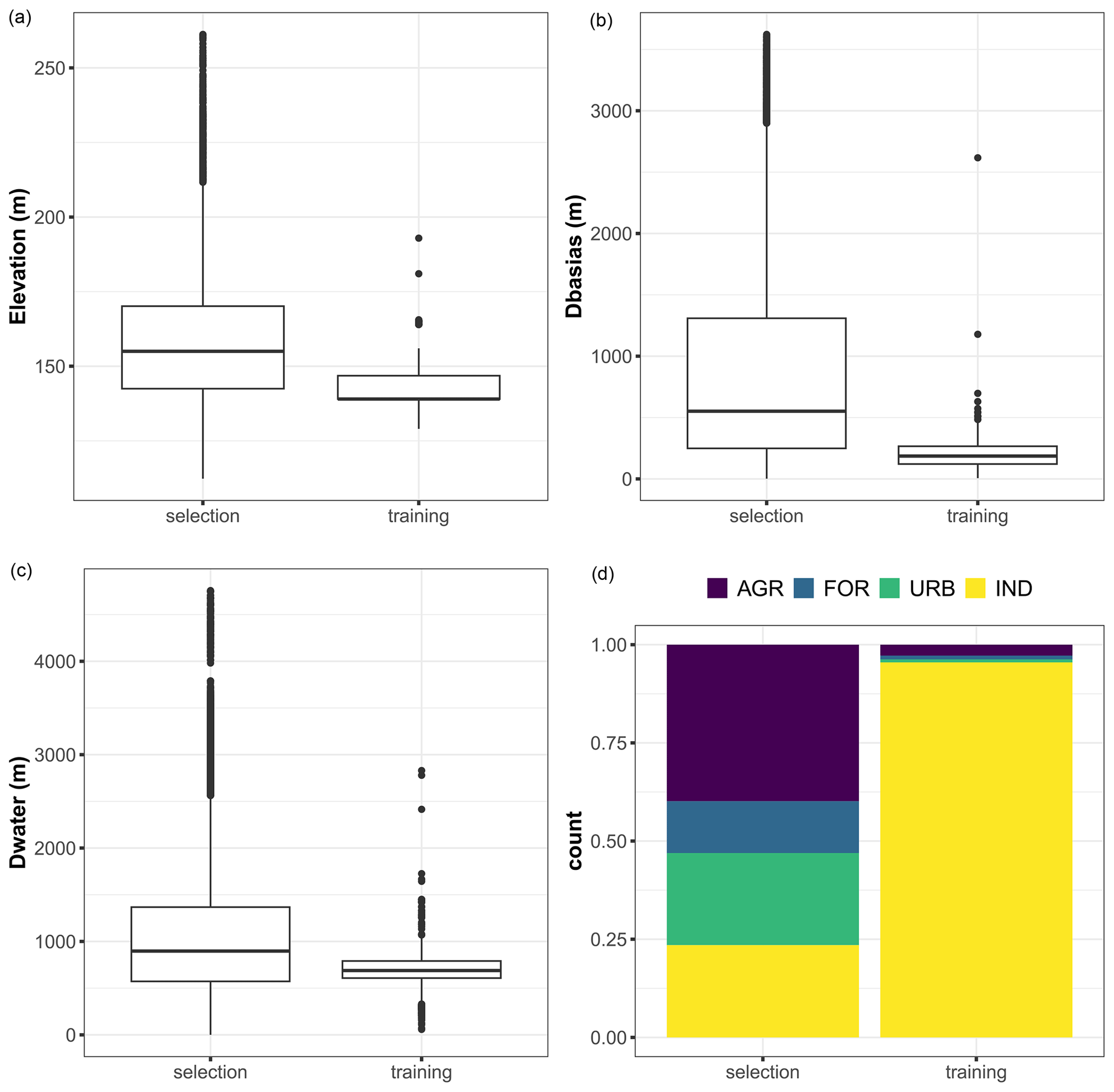
Figure 12 Boxplots of the covariate values for the training dataset and for the locations (named selection) where the corresponding group of covariates significantly contributes to the best estimate, with a scaled Shapley value exceeding that of the uncertainty by more than 25 %. Panel (d) compares the proportions of land use categories (AGR: agriculture, FOR: forests and grasslands, and IND: industrial and commercial economic activities) for the selection and training datasets.

The second situation is the opposite of the first and corresponds to locations where the groups of covariates significantly contribute to the uncertainty, exceeding their contributions to the best estimate by more than 25 %. These are shown in dark green and light red in Fig. 10 (right) and only concern the geographical and D_basias-water groups. In these areas, the RF models predict cases that are well outside the range observed in the training dataset. This is clear for the identified area for the geographical group, which is located outside the spatial domain covered by the soil samples, with the exception of one soil sample located farthest east. An examination of the distributions of the distances D_basias and D_water reveals that the median values exceed those of the training dataset by factors of 10 and 4, respectively (Sect. S2). This indicates that the RF model is being used here beyond the area from which the training data were taken. This is a situation of spatial extrapolations, where tree-based methods such as RF can fail completely; see a recent study highlighting the limitations by Takoutsing and Heuvelink (2022).

Finally, the third situation corresponds to where the covariate groups have negative contributions (outlined in light blue in Fig. 10, right), i.e. where they participate directly in reducing the prediction uncertainty. An examination of the distribution of the corresponding covariates (Sect. S2) indicates the same result as for the first situation, with distances to the nearest rivers even smaller than those observed in the training dataset and with even more marked land use behaviour, where agriculture, forest, and urban are almost the only categories identified. We also note that the geographical group negatively contributes to uncertainty only in the vicinity of the soil samples at distances of 1 to 2 km.

5 Discussion

5.1 Usefulness of the results

To date, the Shapley values have been used to explain individual predictions related to a certain instance of covariates by computing the contribution of each of them to the prediction. Translated for DSM, the Shapley values can be used to determine why a spatial ML model reached a certain value for the soil or chemical properties at a certain spatial location. As discussed by Wadoux and Molnar (2022), the use of Shapley values has the potential to constitute a key tool for environmental soil scientists to improve the interpretation of ML-based DSMs, particularly by providing insights into the underlying physical processes that drive soil variations.

In this study, we complement this type of analysis by addressing the “why” question with respect to the prediction uncertainty, i.e. by explaining why the spatial ML model is confident. For this purpose, the SHAP approach for estimating the Shapley values is applied to decompose the uncertainty indicator provided by the ML spatial model. The attribution results are expected to facilitate communication between environmental soil scientists and stakeholders, which is essential for the inclusion of these new digital soil map products in current practices (see, for example, the discussion by Arrouays et al., 2020). The SHAP results are expected to improve the framing of the prediction results together with the associated uncertainty as illustrated with the synthetic test case described in the introduction as follows: the predicted value of 12.20 is mainly attributable, by a positive factor of almost 50 %, to the maximum and mean temperature of the warmest quarter of the year. The confidence in this result measured by the uncertainty indicator of 1.98 is explained by the diurnal range of almost 50 %. To further increase this confidence, i.e. by decreasing the uncertainty, next efforts should concentrate on the characterisation of this particular covariate.

The second implication of our study is in terms of uncertainty management. Our application to hydrocarbon concentration mapping in Toulouse as well as to the synthetic test case reveals that the determining contributors to the best estimate or the uncertainty may not necessarily be the same. Figure 13 shows maps of the most important groups of covariates with respect to the scaled Shapley absolute values for the real case. These maps show that the prediction uncertainty is dominated by the geographical group over almost 65 % of the entire study area, whereas the best estimate is influenced by this group of covariates over less than 35 %; these areas are outlined in purple in Fig. 13a and b. Overall, the most important group of covariates differs for both prediction objectives over about 50 % of the entire study area (outlined in red in Fig. 13c), mostly in the western and central part of the city. The dichotomy between the drivers of the best estimate and uncertainty is also illustrated for the synthetic test case in Fig. 7.

Figure 13 Spatial distributions of the most important group of covariates with respect to the scaled Shapley values for the prediction best estimate (mean; panel a) and for the prediction uncertainty (IQW; panel b) in the city of Toulouse. Panel (c) shows the regions where the most important group of covariates for the mean agrees with that for IQW. The black squares indicate the locations of the soil samples used for RF training.

On this basis, distinct situations can be identified with different practical implications for data collection and covariate characterisation. This is illustrated in the Toulouse case in Sect. 4.2. If the primary objective of environmental soil scientists is to increase the confidence in the prediction, the characterisation efforts should be concentrated in the zones outside the spatial domain covered by the soil samples, i.e. in regions where the RF models appear to be used to make spatial extrapolations. Two improvements are particularly notable: (1) the modelling of the spatial dependence in the ML model, as revealed by the high importance of the geographical group, and (2) the need for more samples outside the range covered by the soil samples to better characterise the pair of distances D_basias and D_water. On the other hand, if the primary objective of environmental soil scientists is to support the communication of the prediction results to end users, this analysis provides two key elements. First, the results can be explained in the same form as the example provided above by stressing that the predicted pollutant concentration values in the central and western zones of the city are influenced mainly by the covariates that are relevant to the soil prediction problem; different parts of the city being influenced by different groups of covariates (Fig. 11). Second, the results provide evidence for confidence in how the RF model can make predictions, as discussed in Sect. 4.2 based on Fig. 12. Finally, identifying areas where groups of covariates have negative contributions is essential for prioritising actions to reduce prediction uncertainty.

5.2 Applicability to global-scale projects

The application cases analysed in this study correspond to situations with a moderate number of covariates (a few tens) and predictions at either the city scale or the national scale, with several tens of thousands of grid cells, which are representative of other real case situations described in the literature, such as those of Meyer et al. (2018), de Bruin et al. (2022), and Wadoux et al. (2023). In this section, we extend the discussion regarding the applicability to global-scale projects such as that described by Poggio et al. (2021) with hundreds of covariates and millions of grid cells. Applying the SHAP approach is challenging in this context due to its computational load, which is directly related to the number of covariates (Sect. 3.2).

As an illustration, we run SHAP for the Toulouse test case using the nine important covariates (without grouping) at 100 randomly selected grid points (on a Windows desktop x64 with a PC – Intel®Core™ i5-13600H, 2800 MHz, 12 cores, 16 logical processors, with 32 GB physical RAM), which led to an average CPU time of 2.15 s. Given the constraints of global-scale studies, a direct SHAP analysis would require at least 200 d of calculation on a single laptop. The first solution relies on the use of a high-performance computing architecture, as proposed by Wadoux et al. (2023). The second option involves approximating the Shapley values using, for instance, sampling algorithms (Chen et al., 2023), with some approximation errors opposite to those of the exact method used here. The third option explored in this study is the combination of a screening analysis and a grouping approach. Although RF models can handle a large number of covariates, eliminating the covariates before calculating the Shapley values has a clear benefit for saving CPU time. In the real case, the SHAP computational complexity is proportional to 2¹⁵=32 768. The application of screening analysis (Fig. 8) decreases the number of features from 15 to 9, resulting in a relative computational cost reduction of ${\mathrm{2}}^{\mathrm{15}-\mathrm{9}}=\mathrm{64}$. An additional step of grouping is proposed here, with the primary objective of facilitating interpretation. Interestingly, Wadoux et al. (2023) also presented Shapley values for groups of covariates (mean climate, climate extremes, vegetation, topography, etc.) as indicated in Fig. 6 of their study. By grouping before calculating the Shapley values, an additional relative computational cost reduction can be achieved. In the Toulouse case, this implies a cost reduction of ${\mathrm{2}}^{\mathrm{9}-\mathrm{4}}=\mathrm{32}$, and the analysis required less than 1 h for the group-based SHAP (with an average CPU time of 0.054 s). Given the constraints of global-scale studies, this approach here would require less than 7 d of calculation on a single laptop. With the growing concern regarding energy consumption (see, for example, Jay et al., 2024) for scientific computing, this option provides soil scientists with efficient, energy-saving analytical tools, although it requires a careful identification of the covariates of negligible influence as well as the definition of groups.

6 Summary and future work

Providing insights into the uncertainty impacting DSM is a key challenge that requires appropriate diagnostic tools. In an effort to complement the toolbox of environmental soil scientists, in this study, we assessed the feasibility of using the SHAP approach to quantify the contributions of covariates to the machine-learning-based prediction uncertainty at any location in the study area. Using a real case of pollution concentration mapping in the city of Toulouse as well as a synthetic test case, we explored the benefits of jointly analysing the contributors to the prediction best estimate and to the prediction uncertainty. Our results revealed that the drivers of the prediction best estimate are not necessarily the drivers of the confidence in the predictions: this means that decisions in terms of data collection and covariate characterisation may differ depending on the target, the prediction best estimate or the confidence/uncertainty, and the way in which the results of the prediction (and their uncertainty) are communicated.

However, to integrate SHAP at a fully operational level, several lines of improvement need to be considered. First, the implementation to global-scale projects still remains challenging and deserves further work to find a compromise between accuracy, efficiency, and interpretability by paying particular attention to estimation algorithms (Chen et al., 2023), with potential combination with screening and grouping analysis. Second, we focused on a unique uncertainty indicator – namely, the interquartile width – but in some situations, it may not be representative of the total uncertainty, and additional developments are necessary to integrate the entire prediction probability distribution within the SHAP setting. The use of an information-theoretic variant of Shapley values, as investigated by Watson et al. (2023), may be helpful here. Third, we focused on one type of machine learning model, i.e. the quantile RF model. Alternative approaches should be considered in future research: different types of machine learning models, such as deep learning techniques, which have shown promising results (see, for example, Kirkwood et al., 2022), and improved approaches, in particular, to addressing complex sample distributions such as clustering (see, for example, de Bruin et al. (2022) and references therein). Different uncertainty measures should also be tested – for example, geostatistical methods using the kriging variance or statistical quantities derived from stochastic simulations (see, for example, Chilès and Delfiner, 2012), Bayesian techniques (see Abdar et al., 2021, for deep learning techniques), and data-driven approaches such as cross-validation procedures (Ben Salem et al., 2017). These future studies are made possible by the model-agnostic nature of SHAP.

Appendix A: Implementation

The R package ranger developed by Wright and Ziegler (2017) is used to train the RF models as well for the predictions and quantile estimates. The R package sensitivity (https://cran.r-project.org/web/packages/sensitivity/index.html, last access: 25 September 2024) is used to implement the HSIC-based analysis (screening and dependence). The R package shapr developed by Sellereite et al. (2023) is used to implement the group-based SHAP approach. The R package cluster by Maechler et al. (2023) is used to implement the PAM (partitioning around medoids) clustering method. An R markdown based on the vignette of the R package CAST (available at https://hannameyer.github.io/CAST/articles/cast02-AOA-tutorial.html, last access: 25 September 2024) is provided on the GitHub repository at https://github.com/anrhouses/groupSHAP-uncertainty (last access: 25 September 2024).

Appendix B: Quantile random forest

The random forest (RF) model, as introduced by Breiman (2001), is used here for regression. It is a non-parametric technique based on a combination (ensemble named forest) of regression trees (Breiman et al., 1984). Each tree is constructed by relying on recursive partitioning, which aims at finding an optimal partition of the covariates' domain of variation by dividing it into L disjoint sets, R₁, …, R_L, to have homogeneous Y_i values in each set $R_{l=\mathrm{1},\mathrm{\dots },L}$ by minimising a splitting criterion (e.g. based on the sum of squared errors; see Breiman et al., 1984) or when the number of observations in each partition reaches a minimal number termed nodesize (denoted by ns). To sum up, the RF model aggregates the different regression trees as follows: (1) a random bootstrap sample is taken from the training data and m_try variables at each split are randomly selected. Then, (2) n_tree trees T(α) are constructed, where α_t denotes the parameter vector based on which the tth tree is built. Finally, (3) the results from the prediction of each single tree to estimate the conditional mean of Y are aggregated as follows:

$$\begin{array}{}\text{(B1)}& {\displaystyle }\begin{array}{rl}{\displaystyle }Y\left(s\right)& {\displaystyle }=f\left(\mathbf{x}\right(s\left)\right)=\mathrm{E}\left(Y\right|\mathbf{X}=\mathbf{x}\left(s\right))\\ {\displaystyle }& {\displaystyle }={\sum }_{j=\mathrm{1}}^n{w}_j\left(\mathbf{x}\right(s\left)\right)Y_j,\end{array}\end{array}$$

where E(.) is the mathematical expectation and the weight w_j is defined as

$$\begin{array}{}\text{(B2)}& {\displaystyle }\begin{array}{rl}{\displaystyle }{w}_j\left(\mathbf{x}\right(s\left)\right)& {\displaystyle }={\displaystyle \frac{{\sum }_{t=\mathrm{1}}^{n_{\text{tree}}}{w}_t\left(\mathbf{x}\right(s),{\mathit{\alpha }}_t)}{n_{\text{tree}}}},\\ {\displaystyle }& {\displaystyle }\text{with }{w}_j\left(\mathbf{x}\right(s),\mathit{\alpha })={\displaystyle \frac{{\mathrm{I}}_{\mathit{\{}{X}_i\in {\mathrm{R}}_{l(\mathbf{x},\mathit{\alpha })}\mathit{\}}}}{\mathit{\#}\mathit{\{}j:X_i\in {\mathrm{R}}_{l(\mathbf{x},\mathit{\alpha })}\mathit{\}}}},\end{array}\end{array}$$

where I(A) is the indicator operator which equals 1 if A is true and 0 otherwise and R_l(x,α) is the partition of the tree model with parameter α which contains x.

The RF method is very flexible and can be adapted to predict quantiles. The quantile random forest (qRF) model was originally developed by Meinshausen (2006), who proposed to estimate the conditional quantile, q_τ(y|x), at level τ as

$$\begin{array}{}\text{(B3)}& q^{\mathit{\tau }}\left(y\right|\mathbf{x})=\text{inf}(\mathbf{x}:F_{H|\mathbf{X}}\left(y\right|\mathbf{x})\ge \mathit{\tau }),\end{array}$$

where

$$\begin{array}{}\text{(B4)}& F_{Y|\mathbf{X}}\left(y\right|\mathbf{x})={\sum }_{j=\mathrm{1}}^n{w}_j(\mathbf{x}){\mathrm{I}}_{\mathit{\{}{Y}_j\le y\mathit{\}}},\end{array}$$

where the weight is calculated in the same manner as for the regression RF model.

The major difference to the formulation for regression RF is that the qRF model computes a weighed empirical CDF (cumulative distribution function) of Y for each partition instead of computing a weighed average value (as in Eqs. B2–B4).

Appendix C: HSIC dependence measure

The number of covariates is 15 (Sect. 2), which is sufficiently large to pose some difficulties regarding the computational time cost of the SHAP approach (Sect. 3.2). To filter out covariates of negligible influence (screening analysis), we rely on the HSIC (Hilbert–Schmidt independence criterion) measure, which can capture arbitrary dependence between two random variables (potentially of mixed type, continuous or categorical). In the following, we describe the main aspects, and the interested readers can refer to Gretton et al. (2005) and da Veiga (2015).

Let us associate X_i with a universal reproducing kernel Hilbert-Schmidt (RKHS) space defined by the characteristic kernel function k_i(.,.). The same transformation is associated with Y by considering a RKHS space with kernel k(.,.). We define the HSIC measure as follows:

$$\begin{array}{}\text{(C1)}& {\displaystyle }\begin{array}{rl}{\displaystyle }\text{HSIC}& {\displaystyle }(X_i,Y)=\mathrm{E}\left(k_i\right(X_i,X_i^{\prime }\left)k\right(Y,Y^{\prime }\left)\right)\\ {\displaystyle }& {\displaystyle }+\mathrm{E}\left(k_i\right(X_i,X_i^{\prime }\left)\right)\mathrm{E}\left(k\right(Y,Y^{\prime }\left)\right)\\ {\displaystyle }& {\displaystyle }-\mathrm{2}\mathrm{E}\left(\mathrm{E}\right(k_i(X_i,X_i^{\prime })\left|X_i\right)\mathrm{E}\left(k_i\right(Y,Y^{\prime }\left)\right|Y\left)\right),\end{array}\end{array}$$

where $(X_i^{\prime },Y^{\prime })$ is an independent and identically distributed copy of (X_i,Y) and E(.) is the expectation operator.

The role of the characteristic kernel is central here because it can be defined depending on the type of the considered variable. For continuous variables, the Gaussian kernel is used and is defined as $\exp (-\mathit{\lambda }\Vert \mathbf{x}-{\mathbf{x}}^{\prime }{\Vert }^{\mathrm{2}})$, with λ being the bandwidth parameter chosen as the inverse of the empirical variance of the considered variable. For categorical variables, the identity function is used as a characteristic kernel.

The pairwise dependence is measured by $\text{HSIC}(X_i,X_j{)}_{i\ne j}$. To ease the interpretability, the scaled version of Eq. (C1) between 0 and 1 is preferably used – namely, the ratio between HSIC(X_i,X_j) and the square root of a normalising constant equal to $\text{HSIC}(X_i,X_i)\times \text{HSIC}(X_j,X_j)$ as proposed by da Veiga (2015). From the scaled $\text{HSIC}(X_i,X_j{)}_{i\ne j}$, we define the similarity $S(X_i,X_j{)}_{i\ne j}=\mathrm{1}-\text{HSIC}(X_i,X_j{)}_{i\ne j}$.

To perform the screening analysis, we rely on the interpretation of HSIC(X_i,Y) from a sensitivity analysis perspective (da Veiga, 2015) – namely its nullity indicates that X_i does not influence Y. To identify the significant X_i, the null hypothesis ${\mathrm{H}}_{\mathrm{0}}:\text{HSIC}(X_i,Y)=\mathrm{0}$ (against the hypothesis ${\mathrm{H}}_{\mathrm{1}}:\text{HSIC}(X_i,Y)>\mathrm{0}$) is tested, and the corresponding p value can be evaluated (El Amri and Marrel, 2022). When the p value is below a given significance threshold (typically 5 %), it indicates that the null hypothesis should be rejected; i.e. the considered covariate X_i has a significant influence on the variable of interest, Y.