Sensitivity of source sediment fingerprinting to tracer selection methods

In a context of accelerated soil erosion and sediment supply to water bodies, sediment fingerprinting techniques have received an increasing interest in the last 2 decades. The selection of tracers is a particularly critical step for the subsequent accurate prediction of sediment source contributions. To select tracers, the most conventional approach is the three-step method, although, more recently, the consensus method has also been proposed as an alternative. The outputs of these two approaches were compared in terms of identification of conservative properties, tracer selection, modelled contributions and performance on a single dataset. As for the three-step method, several range test criteria were compared, along with the impact of the discriminant function analysis (DFA).

The dataset was composed of tracer properties analysed in soil (three potential sources; n = 56) and sediment core samples (n = 32). Soil and sediment samples were sieved to 63 µm and analysed for organic matter, elemental geochemistry and diffuse visible spectrometry. Virtual mixtures (n = 138) with known source proportions were generated to assess model accuracy of each tracer selection method. The Bayesian un-mixing model MixSIAR was then used to predict source contributions on both virtual mixtures and actual sediments.

The different methods tested in the current research can be distributed into three groups according to their sensitivity to the conservative behaviour of properties, which was found to be associated with different predicted source contribution tendencies along the sediment core. The methods selecting the largest number of tracers were associated with a dominant and constant contribution of forests to sediment. In contrast, the methods selecting the lowest number of tracers were associated with a dominant and constant contribution of cropland to sediment. Furthermore, the intermediate selection of tracers led to more balanced contributions of both cropland and forest to sediments.

The prediction of the virtual mixtures allowed us to compute several evaluation metrics, which are generally used to support the evaluation of model accuracy for each tracer selection method. However, strong differences or the absence of correspondence were observed between the range of predicted contributions obtained for virtual mixtures and those values obtained for actual sediments. These divergences highlight the fact that evaluation metrics obtained for virtual mixtures may not be directly transferable to models run for actual samples and must be interpreted with caution to avoid over-interpretation or misinterpretation. These divergences may likely be attributed to the occurrence of a not (fully) conservative behaviour of potential tracer properties during erosion, transport and deposition processes, which could not be fully reproduced when generating the virtual mixtures with currently available methods.

Future research should develop novel metrics to quantify the conservative behaviour of tracer properties during erosion and transport processes. Furthermore, new methods should be designed to generate virtual mixtures closer to reality and to better evaluate model accuracy. These improvements would contribute to the development of more reliable sediment fingerprinting techniques, which are needed to better support the implementation of effective soil and water conservation measures at the catchment scale.

1 Introduction

During the last several decades, an acceleration of soil erosion has been observed in response to land use changes or farming-practice modifications in several regions around the world (Poesen, 2018; Pennock, 2019). Moreover, global warming will likely further increase the frequency of erosive storms and the associated soil losses (OCC, 2015; Li and Fang, 2016). This acceleration of soil erosion leads to an increase of on-site and off-site negative socio-environmental impacts (Lal, 1998, 2001), including the deterioration of soil agronomic properties (Pimentel, 2006; Montgomery, 2007), the transfer of pollutants associated with soil particles (e.g. pesticides, herbicides, chemical fertilisers, heavy metals, radionuclides) (Lal, 1998; Bing et al., 2013; Debnath et al., 2021), the alteration of soil organic carbon stocks (Olson et al., 2016; Lal, 2019), the degradation of aquatic ecosystems (e.g. eutrophication, increased turbidity) (Kemp et al., 2011; Issaka and Ashraf, 2017) and an increased sediment supply to waterbodies (e.g. reservoir and bay siltation) (Collins et al., 2020). The identification of soil erosion sources is therefore essential to prevent water-erosion-induced land degradation and its associated effects.

The sediment source fingerprinting technique was initially developed to determine the origin of sediment (Wall and Wilding, 1976; Peart and Walling, 1986; Loughran et al., 1987). After initial qualitative studies (Wall and Wilding, 1976; Loughran et al., 1987), the subsequent development of quantitative un-mixing models (Peart and Walling, 1986; Walling and Woodward, 1992; Collins et al., 1997a) made it possible to estimate the contributions of different sources to target sediment samples. Since then, the technique has received increasing attention (Collins et al., 2020; Batista et al., 2022). Overall, the goal of sediment tracing studies has been to improve our understanding of sediment transfer processes and to guide landscape management (Laceby et al., 2015; Owens et al., 2016). However, in practice, the technique has mainly been used by scientists as a research tool, and few direct applications by landscape managers have been reported (Minella et al., 2008; Collins et al., 2020; Xu et al., 2022). This likely demonstrates that, despite some homogenisation and simplification efforts (Mukundan et al., 2012; Collins et al., 2017; Evrard et al., 2022), the technique remains too complex, and the development of simpler and more robust procedures would allow for its wider application (Xu et al., 2022).

In the last few years, there has been a renewed interest among the sediment fingerprinting community in methodological issues associated with the technique, such as the tracer selection methods (i.e. the identification of fingerprint properties suitable for source discrimination and apportionment) (Collins and Walling, 2004; Laceby et al., 2017; Collins et al., 2020; Evrard et al., 2022). This stems from the large diversity of properties that are currently used in sediment fingerprinting studies, e.g. radionuclides (Collins et al., 1997b; Evrard et al., 2020a), elemental geochemistry (Collins et al., 1997b; Blake et al., 2006; Laceby and Olley, 2015), magnetic susceptibility (Lizaga et al., 2019), organic matter and stable isotopes (δ¹³C, δ¹⁵N) (Laceby et al., 2016b; Huon et al., 2018). Collins et al. (2020) listed properties that have recently gained attention, such as compound-specific stable isotopes (CSSIs) (Gibbs, 2008), environmental DNA (eDNA) (Evrard et al., 2019), the stable oxygen isotope ratio with the oxygen isotopic composition of phosphate (δ¹⁸O_p) (Mingus et al., 2019), and diffuse reflectance spectroscopy in the visible (Martínez-Carreras et al., 2010; Summers et al., 2011; Tiecher et al., 2015), near-infrared (Summers et al., 2011) or mid-infrared range (Brosinsky et al., 2014; Farias Amorim et al., 2021). Theoretically, a larger number of measured properties should raise the probability of identifying robust tracers (Laceby et al., 2017; Collins et al., 2020; Evrard et al., 2022). Indeed, tracer selection has a fundamental impact on model predictions and their interpretation (Laceby and Olley, 2015; Laceby et al., 2015; Gaspar et al., 2019), as the inclusion of non-conservative properties in models was shown to strongly decrease the overall model quality (Sherriff et al., 2015; Smith et al., 2018; Vale et al., 2022).

The most conventional approach of tracer selection is a three-step method (TSM) (Collins et al., 2010; Wilkinson et al., 2013; Laceby et al., 2015; Sherriff et al., 2015). The first step assesses the conservative behaviour of each property, and the second step determines their capacity to discriminate between sources. The joint use of both tests allows us to select tracers from a potentially wide suite of measured properties. The third step of this approach consists of selecting optimal tracers for modelling.

Conservative behaviour refers to the absence of changes in the property between sources and targets. Sources correspond to materials that may have contributed to the formation of the target sediments (e.g. land uses, land covers, river banks, roads, landslides). The nature of the target sediments can vary, as it may include material as different as lag sediment, lake sediments, suspended matter, etc. The non-conservative behaviour of a tracer can be mainly attributed to two phenomena. The first is that particle size sorting may occur along the transport pathway (Walling et al., 2000). Sediment transport is a physical mechanism which, depending on runoff magnitude, rainfall intensity, river discharge, and other hydro-sedimentary components, will transport specific particle size fractions, weights and compositions (i.e. mineral or organic fractions) (Viparelli et al., 2013; Gateuille et al., 2019). In general, the average size of particles decreases with the distance travelled (Laceby et al., 2017). Fine particles with a higher specific surface area are generally associated with higher tracer concentrations than coarser material fractions (Horowitze, 1991; Collins et al., 1997a). In order to reduce the impact of particle size sorting on sediment properties, the <63 µm fraction is commonly analysed after sieving both source and target material to this threshold when studying properties preferentially enriched in or sorbed onto fine particles (i.e. clays or silts) (Collins et al., 1997a; Gellis and Noe, 2013; Laceby et al., 2017) such as radionuclides, heavy metals or pesticides (Collins et al., 2020; Evrard et al., 2022). The second phenomenon is related to tracer concentration changes due to biogeochemical processes occurring during particle transport (Koiter et al., 2013). The changes depend on how tracers are affected by biogeochemical processes, such as dissolution, sorption, oxidation and reduction. Highly reactive elements, such as Na, Ca and Mg, show a high water-solubility and tend to dissolve when the sediment is immersed. Other elements, such as Ti, Al and Si, are, in contrast, less susceptible to react in changing conditions (i.e. redox conditions), which makes them more suitable tracers (Meybeck and Helmer, 1989; Phillips and Greenway, 1998).

To assess the conservative behaviour of the property, in the first step of the TSM, the range of property values in source and target samples are compared. The objective of the range test is to assess whether the range of source values includes all individual target sediment sample values (Wilkinson et al., 2013). Various range tests based on source group statistics are commonly used in the literature: minimum–maximum (Smith and Blake, 2014; Sellier et al., 2021), minimum–maximum ± 10 % (as measurement error) (Gellis and Noe, 2013; Gellis and Gorman Sanisaca, 2018; Dabrin et al., 2021), boxplot examination (whiskers and hinge box) (Sellier et al., 2020; Batista et al., 2022), mean (Wilkinson et al., 2013; Nosrati et al., 2021), mean plus/minus standard deviation (SD) (Evrard et al., 2020b; Laceby et al., 2021) and median (Collins et al., 2013; Batista et al., 2022). In these range tests, the source property range is defined as the highest and lowest values of the chosen statistics among the source groups. However, range tests do not quantify or confirm the complete absence of non-conservative behaviour (Collins et al., 2017; Sherriff et al., 2015).

The property's ability to differentiate between sources, originally proposed by Collins et al. (1997b), determines whether a property is a discriminant tracer or not. This second step of the TSM allows for the selection of tracers that maximise source discrimination. To assess the discrimination power of a given property, the conventional tracer selection approach relies on the non-parametric Kruskal–Wallis H test (Hollander et al., 2013). The result of the Kruskal–Wallis H test indicates that at least one of the groups differs from the other for a given property. Other tests, such as Dunn's, Mann–Whitney U or Kolmogorov–Smirnov tests, can be used to determine the discriminatory power of a given property for each individual source (e.g. forest versus cropland versus subsoil).

Conventionally, after assessing the tracer's conservative behaviour and discrimination capacity, the third step of the TSM is to conduct a discriminant function analysis (DFA) or a principal component analysis (PCA). When applying the DFA, a subset of tracers is selected using a forward stepwise selection procedure based on Wilk's lambda criterion (Collins et al., 1997b). This step aims at selecting the lowest number of tracers that maximises sample source discrimination, in order to avoid selecting redundant tracers (Small et al., 2004). However, this practice is currently debated, as some authors argue that a higher number of tracers can improve source dimensionality and definition, as well as alleviate the impact of non-conservative tracers (Martínez-Carreras et al., 2008; Sherriff et al., 2015).

Another tracer selection method, the consensus method (CM), was developed by Lizaga et al. (2020). It is based on the information provided by single tracers in an un-mixing context. The CM selects tracers combining the identification of non-conservative behaviour and conflicting tracers. It consists of two tests: the conservativeness index (CI) and the consensus ranking (CR). The CI is based on the results of the predictions from single-tracer models to identify non-conservative and dissenting tracers, whereas the CR is a scoring function based on debates aimed at discarding the properties that prevent consensus. The CI is applied to all target sediment samples and provides unique results for the entire study, whereas the CR is applied to each individual target sediment sample, which may result in the selection of different lists of tracers for different target samples.

Selected tracers are then used in un-mixing models to assess the contribution of sources to the target samples. After the use of simple (Peart and Walling, 1986) and quantitative un-mixing models (Collins et al., 1997a), earlier modelling approaches were based on deterministic optimisation procedures (Walden et al., 1997), and, more recently, more advanced approaches have moved towards stochastic procedures using Bayesian and/or Monte Carlo methods (Small et al., 2002; Martínez-Carreras et al., 2008; Nosrati et al., 2014; Laceby and Olley, 2015). In order to assess the overall reliability of the study, it is important to assess the predictive accuracy of the un-mixing models. Stochastic models produce a distribution of source contributions for which a prediction interval can be determined, which provides an indicator of modelling accuracy (Batista et al., 2022). The use of artificial mixtures allows prediction accuracy to be assessed in more diverse ways by using them as target mixtures with known contributions. It is then possible to calculate various statistics to describe and evaluate the prediction uncertainty. Although these mixtures were initially prepared in the laboratory (Martínez-Carreras et al., 2010; Haddadchi et al., 2014; Huangfu et al., 2020), the development of virtually generated mixtures (Laceby et al., 2015; Palazón et al., 2015; Sherriff et al., 2015) appears as a relevant alternative (Batista et al., 2022). However, when artificial mixtures are produced, their properties are not affected by erosive processes and are therefore perfectly conservative.

The objectives of the current study are therefore to (1) compare the tracer selections given by the two approaches (i.e. three-step method and consensus method), (2) assess the impact of the stepwise selection on the TSM selections of tracers, (3) evaluate the impact of these different selections of tracers on sediment source apportionment prediction accuracy using virtual mixtures and (4) draw general recommendations from this evaluation for future sediment fingerprinting studies.

2 Materials and methods

2.1 Catchment description

The Hayama Lake catchment (84 km²), located in the upper part of the Mano River in northeastern Japan (Fukushima Prefecture, Tōhoku region), is a typical mountainous agricultural catchment of the eastern edge of Fukushima Prefecture. Due to the steep topography, cropland is located at the bottom of valleys and in the vicinity of rivers, and it is bordered by forest on steep mountainous hillslopes. Forestry is the main land use, which covers 91 % of the catchment, while cropland represents 7 % and urban settlements and bare soil less than 2 % (Fig. 1 and Fig. B1 in Appendix B; data are from JAXA, 2016, 2018, 2022). However, cropland is located in places with a high hydro-sedimentary connectivity (Chartin et al., 2013). The Hayama Lake catchment area is located within the main inland radioactive contamination plume resulting from the Fukushima Daiichi Nuclear Power Plant accident in March 2011 (Kato et al., 2019). Once deposited, ¹³⁷Cs strongly and quasi-permanently binds to fine soil particles such as silts and clays (Sawhney, 1972; He and Walling, 1996), which has been confirmed in the soils of Fukushima Prefecture (Saito et al., 2014; Nakao et al., 2014).

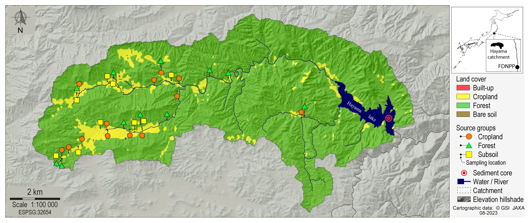
Figure 1 Map of the main land uses in the Hayama Lake catchment area over the 2014–2016 period with location of source samples and the sediment core (cartographic data: GSI and JAXA). FDNPP: Fukushima Daiichi Nuclear Power Plant.

Catchment altitude ranges from 170 to 700 m above sea level. The climate is continental (Dfa), with no dry season and hot summer, and it is bordered to the east by a Cfa temperate climate with no dry season and hot summer according to Köppen's climatic classification (Beck et al., 2018). The regional hydrological year runs from November to October (Laceby et al., 2016a; Whitaker et al., 2022). Over the 2006 to 2021 period, the mean annual temperature was 13.6±0.4 ^∘C yr⁻¹ (standard deviation), with mean monthly values ranging from −1.5 ^∘C in January to 31.1 ^∘C in August. The mean annual precipitation was 1220±189 mm yr⁻¹ (SD), some of which falls as snow in winter. The majority of precipitation occurs between June and October, representing 60 % of the annual rainfall and 86 % of the rainfall erosivity (Laceby et al., 2016a). This period corresponds to the Japanese typhoon season with a peak of intensity in September in Fukushima Prefecture. Major typhoons were shown to be the main drivers of sediment production (Chartin et al., 2017), as they can generate 40 % of the annual rainfall erosivity within a very short period (Laceby et al., 2016a).

The Hayama Lake catchment is mainly underlain by non-alkaline mafic volcanic rocks (42 %), granite (31 %) granodiorite (17 %) and sedimentary rocks (7 %) (Fig. B2). Main soil groups, according to the Comprehensive Soil Classification System of Japan (Obara et al., 2011, 2015, and equivalent soil types according to the World Reference Base for Soil Resources (WRB)), are the following: Brown Forest soils (37 %; WRB: Cambisols/Stagnosols), Allophanic Andosols (36 %; Silandic Andosols), Cambic Red-Yellow soils (9 %; WRB: Cambisols) and Lithosols (9 %; WRB: Leptosols) (Fig. B3) (data from NARO, 2011).

All maps and geographical processing were performed using the QGIS software (QGIS Development Team, 2022).

2.2 Soil and sediment sampling and processing

All sediment targets were taken from one sediment core sampled on 8 June 2021 in the downstream part of Hayama Lake (Mano dam lake) at 42 m depth (Fig. 1) by the National Institute of Environmental Studies (NIES) (Japan). The core was 38 cm long with a diameter of 11 cm. It was sectioned into 38 increments of 1 cm in order to achieve a high-resolution investigation of the sediment core. A group of 32 layers were selected for this study, from 6 to 38 cm depths, which corresponds to a stable land use period (i.e. prior to decontamination work; Chalaux-Clergue et al., 2024). Sediment samples were dried at 40 ^∘C for 96 h.

Soil samples (n = 56) were collected in areas representative of the main potential sediment sources to Hayama Lake, including 24 cropland, 22 forest and 10 subsoil (i.e. channel bank or landslide) samples. Some source soils were sampled in the adjacent Niida River catchment, which is similar to the Hayama Lake catchment. Particular care was taken to ensure that these samples were representative of the Hayama Lake catchment characteristics, in terms of land use, geology and pedology (see Figs. B1, B2 and B3) (Williamson et al., 2023). The similarity of soil sample properties from both catchments was tested using the Kolmogorov–Smirnov test (not shown). Soils were sampled with a plastic trowel and consisted of 10 composited sub-samples of topsoil (1–2 cm uppermost layer). All soil samples were dried at 40 ^∘C for about 48 h and then sieved to 63 µm to isolate the fraction concentrating ¹³⁷Cs (i.e. to silt and clay minerals (Sawhney, 1972; He and Walling, 1996)).

2.3 Laboratory analysis

Various analyses were conducted to characterise sediment and soil properties: organic matter composition determined by the combustion method (i.e. total organic carbon (TOC) and total nitrogen (TN)), elemental geochemistry analysed by X-ray fluorescence (XRF) for 17 elements (i.e. Al, Ca, Co, Cr, Cu, Fe, K, Mg, Mn, Ni, Pb, Rb, Si, Sr, Ti, Zn and Zr), visible colour indices by diffuse reflectance (i.e. CIE Lab, CIE LCh), geothite peak intensities (445 and 525 nm; Tiecher et al., 2021), the ratio between the % reflectance at 700 and 400 nm (Q7/4; Debret et al., 2011) and iron oxide-associated parameters (A1, A2, A3, Gt; Tiecher et al., 2015). All analysis methods and calculations are described in Appendix C.

Only properties for which the measurement uncertainty is too large were removed from further analysis. The following criterion has been set: if obtaining, considering the measurement uncertainty, a majority or the totality of the sample values was virtually impossible (e.g. when the measurement uncertainty is subtracted from the property measurement and results in a negative value), then the corresponding property was discarded.

2.4 Virtual mixtures

Virtual mixtures were generated in order to assess model prediction accuracy (Palazón et al., 2015; Smith et al., 2018; Gaspar et al., 2019; Farias Amorim et al., 2021; Batista et al., 2022). They were shown to provide a reliable alternative to laboratory mixtures (Batista et al., 2022). Their ease of generation allows the model to be evaluated under a wide range of source contributions. For a given source, virtual mixture contributions were designed to range from 0 % to 100 %, with 5 % increments. The contributions of the other sources to the mixtures were then determined as fractions of the remaining contribution (i.e. 1 − source A contribution), the fractions being in turn determined by the number of sources. The denominators were defined as $(n-\mathrm{1})\cdot \mathrm{2}$ with n the number of source. The numerators were set to 3 and 1 as three sources were considered in the current research ($\mathrm{3}/\mathrm{4}$ and $\mathrm{1}/\mathrm{4}$). Theoretical source contributions for the virtual mixtures were determined as follows:

$$\begin{array}{}\text{(1)}& (C_A,C_B,C_C)=\left\{\begin{array}{l}{C}_A\in \mathit{\{}\mathrm{0},\mathrm{5},\mathrm{\dots },\mathrm{100}\mathit{\}},\\ C_B=(\mathrm{1}-C_A)\cdot \frac{\mathrm{3}}{(n-\mathrm{1})\cdot \mathrm{2}},\\ C_C=(\mathrm{1}-C_A)\cdot \frac{\mathrm{1}}{(n-\mathrm{1})\cdot \mathrm{2}},\end{array}\right.\end{array}$$

with C_A, C_B and C_C being the contributions of sources A, B and C, and n is the number of sources.

Permutations were then determined following this contribution scale, which generated a total of 138 virtual mixtures for the three source groups. For every source group, the mean and SD of each property were calculated. For each virtual mixture, each source group mean value was multiplied by the corresponding group contribution (e.g. cropland 0.40, forest 0.45, subsoil 0.15). Then, all source group values were summed to provide the virtual mixture property value.

2.5 Tracer selection

2.5.1 Three-step method

The TSM (Mukundan et al., 2010; Sellier et al., 2020; Batista et al., 2022) is based on three steps: (1) a range test to identify conservative properties (Martínez-Carreras et al., 2010; Wilkinson et al., 2013; Gellis and Walling, 2013), (2) a Kruskal–Wallis H test to identify discriminant properties (Collins et al., 1997b), and then (3) a discriminant function analysis (DFA) or a principal component analysis (PCA) with forward stepwise selection based on Wilk's lambda criterion to identify the best subset of predictors among the identified tracers (i.e. conservative and discriminant properties) (Collins and Walling, 2002).

Conservative behaviour

The conservative behaviour of properties was assessed using a range test. Within a range test, the range of sources is defined as the highest and lowest values of a criterion of the property among source groups. To be conservative, all the sample property values should lie within the source range.

$$\begin{array}{}\text{(2)}& \begin{array}{rl}\text{conservative if}& \mathit{\{}\text{sources lower bound}\le \text{target value}\\ & \le \text{sources upper bound}\mathit{\}}\end{array}\end{array}$$

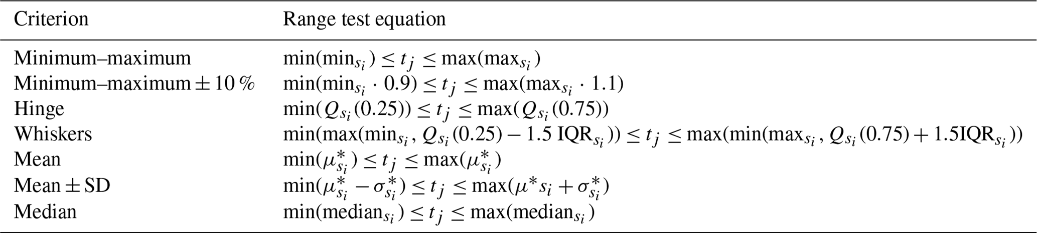
Several range test criteria are found in the literature, and these were all applied to identify conservative properties as an alternative to the TSM: minimum–maximum (Smith and Blake, 2014; Sellier et al., 2021), minimum–maximum ± 10 % (as measurement error) (Gellis and Noe, 2013; Gellis and Gorman Sanisaca, 2018; Dabrin et al., 2021), boxplot whiskers interpretation (i.e. outlier thresholds) (Sellier et al., 2020) and boxplot hinge interpretation (i.e. also referred to as interquartile range (IQR)) (Batista et al., 2022), mean (Wilkinson et al., 2013; Nosrati et al., 2021), mean plus/minus 1 standard deviation (mean ± SD) (Evrard et al., 2020b; Laceby et al., 2021), and median (Collins et al., 2013; Batista et al., 2022) are detailed in Table 1.

Table 1 Equations of the common range test criteria used in the literature to test the conservative behaviour in the three-step method (TSM). s_i is the source group i from 1 to n, the number of source groups; t_j is the target sample j value with j from 1 to m, the number of samples; and μ is the mean and σ is the standard deviation (SD). Symbol ^* indicates statistics calculated on log-transformed values.

Discriminant power

The ability of the property to discriminate between source groups is assessed using a Kruskal–Wallis H test (Hollander et al., 2013). This is a non-parametric test that checks whether two or more samples originate from the same distribution, and it represents an extension of the Mann–Whitney U test that compares two samples. The test hypotheses are the following.

• The null hypothesis (H₀): the median across the three groups are equal.

• The alternative hypothesis (H₁): at least one of the group medians is different from the others.

The test statistic is given by

$$\begin{array}{}\text{(3)}& H=(N-\mathrm{1}){\displaystyle \frac{\sum _{i=\mathrm{1}}^g{n}_i({\stackrel{\mathrm{‾}}{r}}_i-\stackrel{\mathrm{‾}}{r}{)}^{\mathrm{2}}}{\sum _{i=\mathrm{1}}^g\sum _{j=\mathrm{1}}^{n_i}(r_{ij}-\stackrel{\mathrm{‾}}{r}{)}^{\mathrm{2}}}},\end{array}$$

with N being the total number of observations across all groups, g the number of groups, n_i the number of observations in group i, r_ij the rank of observation j from group i, ${\stackrel{\mathrm{‾}}{r}}_i$ the mean rank of all observations for group i and $\stackrel{\mathrm{‾}}{r}$ the mean of all r_ij.

Kruskal–Wallis H tests were performed using the function kruskal.test from the stats package (R Team, 2022). For properties with a p value below α = 0.05, the null hypothesis is rejected, which means that at least one of the source groups is different from the others and that the property is therefore discriminant.

Discriminant function analysis

A discriminant function analysis (DFA) stepwise selection is carried out to identify a subset of predictors among the identified tracers (Collins and Walling, 2002; Collins et al., 2010). A forward stepwise variable selection based on Wilk's lambda criterion was performed using the function greedy.wilks from the klaR package (Weihs et al., 2023). The function first initiates a model with the variable that discriminates groups. Then, the model is extended by including other variables based on Wilk's lambda criterion: the one variable that minimises the Wilk's lambda is only included if the model's p value remains statistically significant after its inclusion. Wilk's lambda statistic approaches zero when the variability between groups is higher than the variability within each group; then this criterion maximises the difference between groups. As the use of the DFA stepwise selection has been criticised because some studies showed that the use of a higher number of tracers decreases the sensitivity of the results to non-conservative tracers (Martínez-Carreras et al., 2008; Sherriff et al., 2015), we used the list of identified tracers before (“no DFA”) and after the stepwise selection procedure (“DFA”) in order to assess its potential impact on the calculation of source contributions.

2.5.2 Consensus method

The approach by Lizaga et al. (2020) to select properties, referred to as the consensus method (CM), is based on two tests: the conservativeness index (CI) and the consensus ranking (CR). In the CM, tracers are selected by identifying non-conservative behaviour (using the CI test) and dissenting tracers (CR test). The CI of each property is calculated for all target samples simultaneously, while the CR is calculated for each target sample independently. As a result, a set of tracers is selected for each target sample. Tests were performed using the 1.3 version of FingerPro (Lizaga et al., 2022) under the R ver. 4.1.2 (R Team, 2021) environment.

Conservativeness index

The CI quantifies how conservative a property is based on the result of a single-tracer model. To be considered conservative, the CI should be strictly equal to 0. A single-tracer model is a standard linear un-mixing model with only one true analysed property and n−2 virtual properties (n the number of source groups). The model is solved to obtain the source contributions. This process is repeated 2000 times, which creates a distribution of predictions. The prediction couples (i.e. $w_{\mathrm{1}},w_{\mathrm{2}},\mathrm{\dots },w_n$) are sorted according to the Euclidean distance to a perfectly balanced mixture (i.e. $\mathrm{1}/n$). A percentile of the sorted prediction couple is chosen to compute the CI as the root mean square error (RMSE) of the non-conservative part (nc) of the contribution, as follows:

$$\begin{array}{}\text{(4)}& \begin{array}{rl}& \mathrm{CI}=-\sqrt{\sum _{j=\mathrm{1}}^n\left(\mathrm{nc}\right(w_j)-{\displaystyle \frac{\mathrm{1}}{n}}{)}^{\mathrm{2}}};\mathrm{with}\\ & \mathrm{nc}\left(w\right)=\left\{\begin{array}{ll}-w& \mathrm{if}w<\mathrm{0},\\ \mathrm{0}& \mathrm{if}\mathrm{0}⩽w⩽\mathrm{1},\\ w-\mathrm{1}& \mathrm{if}w>\mathrm{1},\end{array}\right.\end{array}\end{array}$$

with w_j being of the jth source group predicted contribution of the selected percentile, and n is the number of source groups.

A property is considered conservative if the CI values are strictly equal to zero.

Consensus ranking

CR is an index that quantifies the relevance of each property for the prediction based on a debate agreement for a single target sample. In each debate, a subset of n+1 randomly selected properties is built, and several rounds of debates are performed excluding one property each time. The consensus of each debate is measured through the quality of the mass balance equations. When the exclusion of a property leads to an increase of the subset consensus score (i.e. higher RMSE of the mass balance equations), the property is considered dissenting and “lost a debate”. The CR of a property is the ratio between the number of attended debates (set at 2000) and the number of lost debates, and it is calculated as follows:

$$\begin{array}{}\text{(5)}& \mathrm{CR}=\mathrm{100}(\mathrm{1}-{\displaystyle \frac{\text{lost debates}}{\text{attended debates}}}).\end{array}$$

Properties with a CR score above a certain threshold are considered relevant and are selected. Lizaga et al. (2020) recommended to select properties with a CR score above 70.

2.6 Source contribution modelling

2.6.1 Un-mixing model

An un-mixing model was run on actual sediment samples and virtual mixtures using the tracers selected by the TSM without and with DFA and the CM. To do so, the widely used Bayesian un-mixing model MixSIAR was employed using the R package MixSIAR (Stock et al., 2020, ver. 3.1.12) with JAGS (Stock et al., 2022, ver. 4.3.1) (Collins et al., 2020; Evrard et al., 2022; Lizaga et al., 2020; Batista et al., 2022). To quantify the contributions of n sources, the model requires n−1 tracers. The model was run with a “long” Markov Chain Monte Carlo sampling algorithm (i.e. chain length = 300 000, burn-in = 200 000, thin = 100 and chains = 3) with a process error structure. Model convergence was determined by the Gelman–Rubin diagnostic using the output_JAGS function from the MixSIAR package, and none of the tracer selection approaches tested had a value greater than 1.05. The median value of the distribution predicted by MixSIAR was reported as the source contribution for each sediment target and virtual mixture.

2.6.2 Accuracy assessment

For each tracer selection approach, MixSIAR prediction accuracy was assessed using virtual mixture contribution predictions, for which theoretical source contributions were known a priori. Each model's prediction accuracy was evaluated based on different criteria: uncertainty (prediction interval width (W50)), residual error or bias (mean error (ME)), performance (squared Pearson correlation coefficient (r²)), root-mean-square error (RMSE), Nash–Sutcliffe modelling efficiency coefficient (NSE), and continuous ranked probability score (CRPS). A summary of the metrics, with their formula, unit, range and ideal values, is provided in Table 2 (Matheson and Winkler, 1976; Bennett et al., 2013; Batista et al., 2022).

Table 2 Formula of model prediction accuracy metrics. With z_i and ${\widehat{z}}_i$, respectively, the measured and predicted contributions for the sample i; $\stackrel{\mathrm{‾}}{z}$ and $\stackrel{\mathrm{‾}}{\widehat{z}}$ the measured and predicted mean contribution of all samples; and n the number of samples.

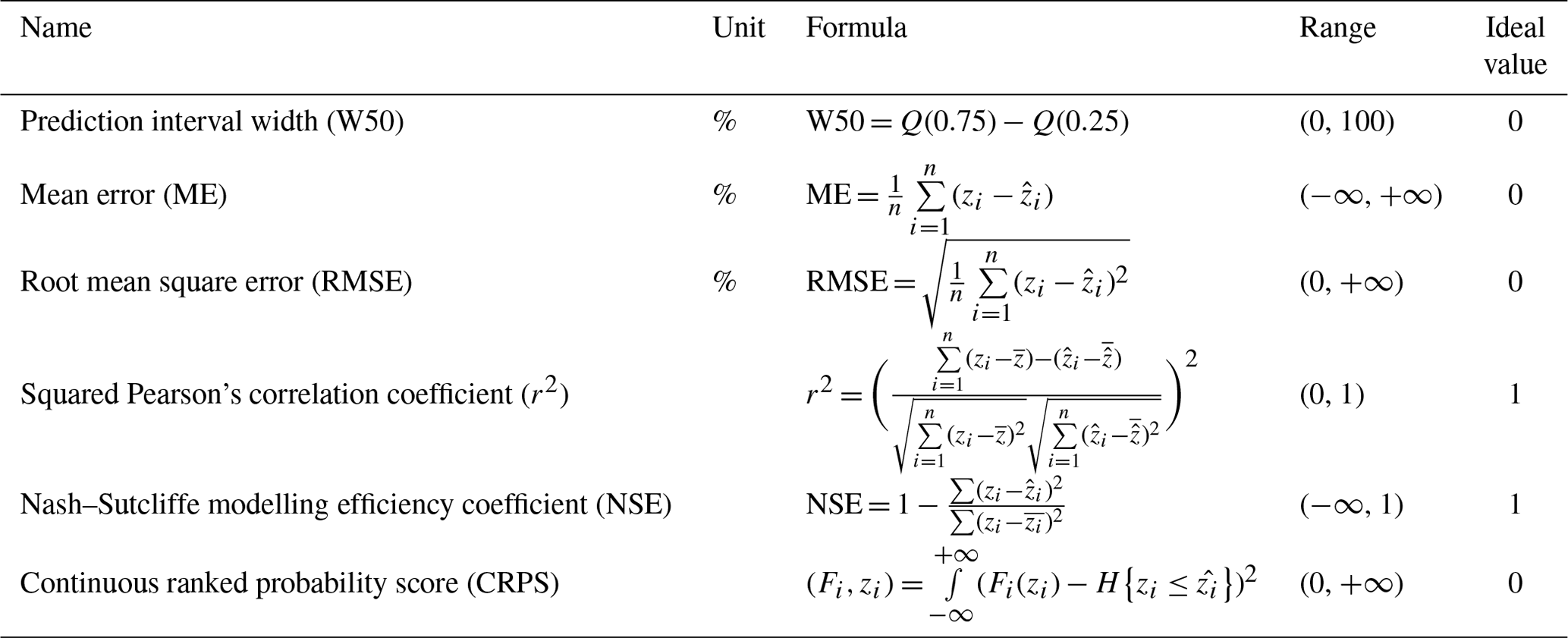
Higher values of W50 indicate a wider distribution, which is related to a higher uncertainty. The sign of the ME indicates the direction of the bias, i.e. an overestimation or underestimation (positive or negative value, respectively). As ME is affected by cancellation, a ME of zero can also reflect a balanced distribution of predictions around the 1 : 1 line. Although this is not a bias, it does not mean that the model outputs are devoid of errors. The RMSE is a measure of the accuracy and allows us to calculate prediction errors of different models for a particular dataset. RMSE is always positive, and its ideal value is zero, which indicates a perfect fit to the data. As RMSE depends on the squared error, it is sensitive to outliers. The r² describes how linear the prediction is. The NSE indicates the magnitude of variance explained by the model, i.e. how well the predictions match with the observations. A negative RMSE indicates that the mean of the measured values provides a better predictor than the model. The joint use of r² and NSE allows for a better appreciation of the distribution shape of predictions and thus facilitates the understanding of the nature of model prediction errors. The CRPS evaluates both the accuracy and sharpness (i.e. precision) of a distribution of predicted continuous values from a probabilistic model for each sample (Matheson and Winkler, 1976). The CRPS is minimised when the observed value corresponds to a high probability value in the distribution of model outputs. The formulae and the full description of this score are available in Jordan et al. (2019) and Laio and Tamea (2007). The calculation of the CRPS was performed using the crps_sample function from the scoringRules package (Jordan et al., 2019). Model global CRPS^* and W50^* value are calculated as the mean of individual CRPS and W50 values, respectively. In addition to the metric values, a graphical evaluation of model predictions was performed through plotting observed versus predicted CRPS sample values and W50 sample values for each source group.

All data analyses were performed using R (R Team, 2022, ver. 4.2.2) within RStudio (RStudio Team, 2022). An R package (fingR) implementing the approach followed in this study was developed and is freely available (Chalaux-Clergue and Bizeul, 2023).

3 Results

According to the measurement uncertainty criterion (Sect. 2.3), the following properties were removed from subsequent analysis: the elemental concentrations in Co, Cr, Cu, Ni and Rb; the visible colorimetric index A3, and the goethite peak at 445 nm (G₄₄₅), as their measurement uncertainties were too high.

3.1 Tracer selection

3.1.1 Selection of tracers

Three-step method

The different range tests resulted in unique sets of conservative properties, with only TN and Q7/4 passing all tests (Fig. 2). Nevertheless, the majority of tests identified TOC, G₅₂₅, b^*, Al, Ti, L^* and C^* (Table 3) as being conservative. The minimum–maximum ± 10 % is the range test criterion that identified the highest number of properties (n=19), followed by the minimum–maximum (n=16) and whiskers (n=12). The minimum–maximum ± 10 % range test criterion was the only one that identified Fe, Pb, h, A1 and GT. As the minimum–maximum criterion, this test identified Ca, K, Mg and Sr as conservative. The mean and median criteria identified only three (TN, b^*, Q7/4) and four properties (TOC, TN, Q7/4, G₅₂₅), respectively. Among the properties identified as conservative, Fe, Mg, Pb and Ti were not identified as discriminant by the Kruskal–Wallis H test (p value = 0.08) and were therefore removed from the list of potential tracers. Although a majority of tests identified Ti as conservative, only the minimum–maximum ± 10 % criterion identified Fe, Mg and Pb as conservative. The DFA procedure mostly resulted in the systematic exclusion of A2 and in the frequent exclusion of TN and G₅₂₅, while TOC, Al, Si, L^* and Q7/4 were retained by most of the range test criteria. Among the 16 tracers selected by the minimum–maximum criterion, the DFA discarded seven of them (TN, Ca, Sr, b^*, C^*, A2 and G₅₂₅). In contrast, for the minimum–maximum ± 10 % criterion that selected 19 tracers, only five tracers (i.e. TOC, TN, Ca, A2 and G₅₂₅) were discarded by the DFA. The outputs of the mean and median criteria were not modified by the DFA.

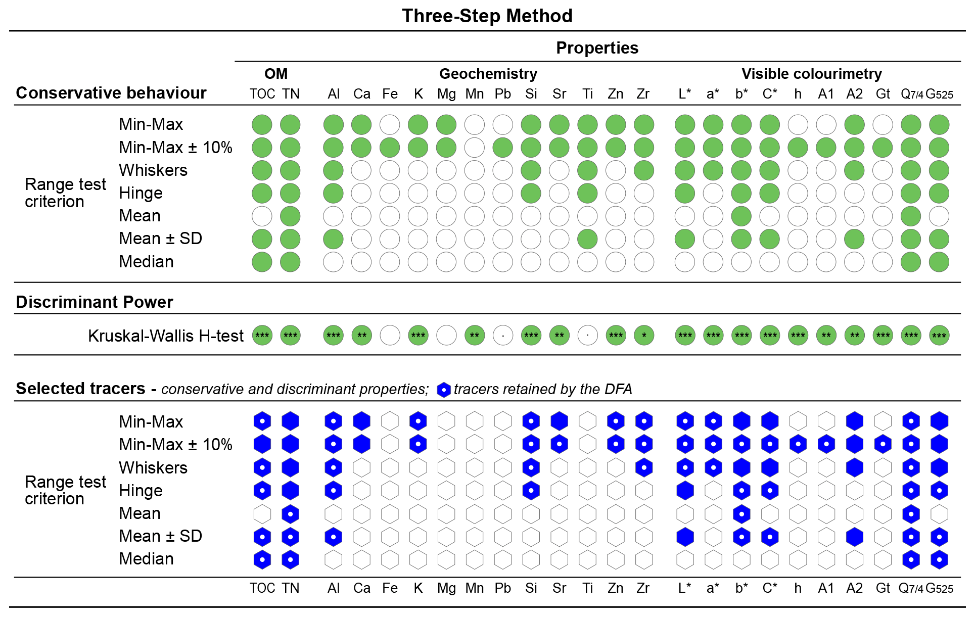
Figure 2 Tracer selection using the three-step method (TSM) according to different range test criteria. Green filled circles indicate a property that passed the conservative behaviour (i.e. range test) or the discriminant power (Kruskal–Wallis H test) tests. Blue filled diamonds indicate selected tracers (i.e. properties that passed both conservative behaviour and discriminant power tests) and blue diamonds with white points indicate tracers retained by the discriminant function analysis (DFA) forward stepwise selection based on Wilk's lambda criterion. Kruskal–Wallis H test's p-value significance: “${}^{***}$” p value < 0.001; “${}^{**}$” p value < 0.01; “^*” p value < 0.05; “.” p value < 0.1; “ ” p value < 1. OM: organic matter; Min–Max: minimum to maximum; SD: standard deviation.

Consensus method

The CI values indicate that TOC, TN, b^* and C^* were identified as conservative properties (CI strictly equal to 0, Fig. 3) However, Al, Si, Ti, Q7/4 and G₅₂₅ obtained a CI very close to zero (i.e. −0.1), whereas it was equal to −0.2 for Zn, L^* and A2. For these four properties, all sediment samples (n = 32) obtained a CR score above the threshold (i.e. 70) for all sediment samples (i.e. 32 out of 32) and were therefore considered relevant and kept in the list of tracers for further analysis. In addition, properties which obtained CI values close to zero (i.e. Al, Si, Ti, Q7/4, G₅₂₅, Zn, L^* and A2) also reached a high CR score (i.e. respectively 25, 22, 30, 25, 32, 24, 16 and 20).

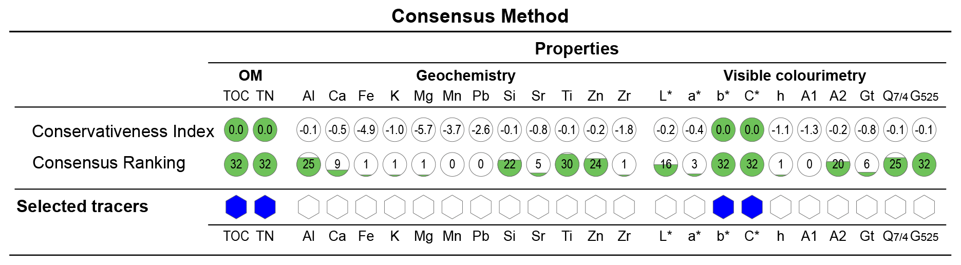
Figure 3 Tracer selection using the consensus method (CM). Green filled circles indicate properties selected by the conservativeness index (i.e. CI = 0.0). The value in the circle refers to the number of sediment samples (out of 32) that obtained a Consensus Raking score above the threshold (i.e. CR ≥ 70). Blue filled diamonds indicate selected tracers. OM: organic matter.

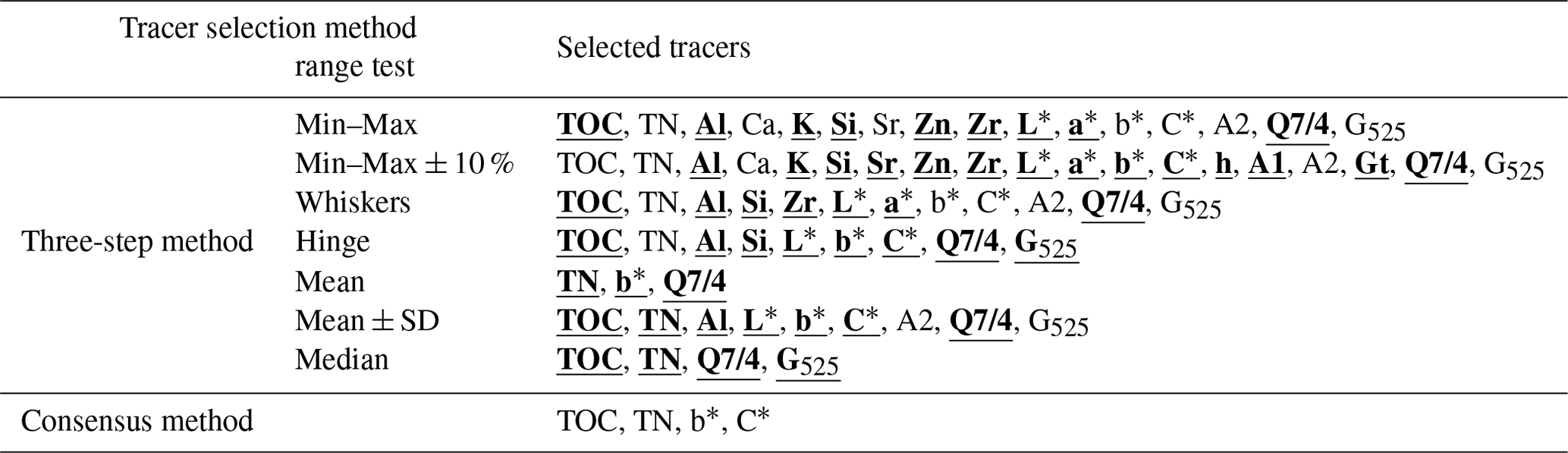
Table 3 summarises the list of tracers selected by each approach.

Table 3 Tracers selected by the three-step method (TSM) according to the range test criteria and the consensus method (CM). Tracers underlined and written in bold were retained by the discriminant function analysis (DFA) forward stepwise selection based on Wilk's lambda criterion. Min–Max = minimum to maximum.

3.2 Prediction accuracy and tracer selection methods

The sediment source apportionment prediction accuracies obtained when using the mean range test criterion and CM for tracer selection were lower compared to that obtained when using the other TSM range test criteria (Fig. 4 and Tables A1, A2, A3 and A4 in Appendix A). However, the difference in prediction accuracy was greater between sources within each tracer selection method than between methods (i.e. TSM and CM). The effect of the DFA stepwise selection was to mainly modify the prediction accuracy of cropland and forest. On average, W50^* values (+20 %), r² (+0.01) and NSE (+0.04) increased, while ME (−37 %), RMSE (−8 %) and CRPS (−1) decreased. In short, uncertainty increased (W50^*), bias decreased (ME) and performance slightly increased (r², NSE, CRPS^*) when the DFA was applied.

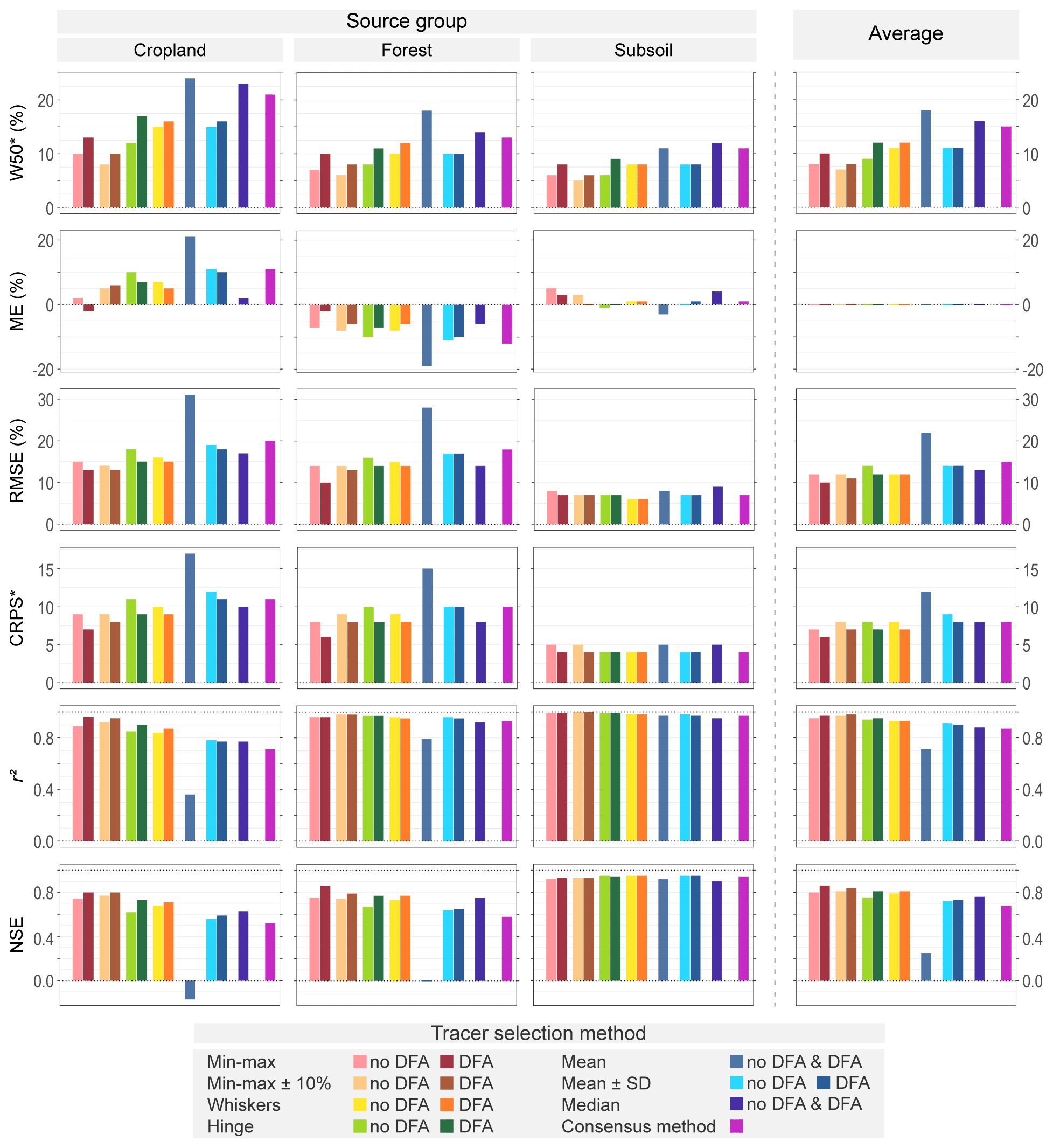
Figure 4 Summary of MixSIAR accuracy statistics calculated on virtual mixtures (n = 138) for each tracer selection method: three-step method (TSM) range test criteria and consensus method (CM) for each individual soil source and average of all three sources for each method. Tracers selected by each method are listed in Table 3. Model accuracy statistics were shown by darker bar plots for each selection approach. W50^*: prediction interval width; ME: mean error; RMSE: root mean square error; r²: squared Pearson's correlation coefficient; NSE: Nash–Sutcliffe modelling efficiency coefficient; CRPS: continuous ranked probability score. Note that symbol ^* indicates mean values per source.

Regardless of the tracer selection method, the W50^* values indicate a higher uncertainty for cropland, followed by forest and subsoil (Fig. 4). The CM, mean and median range test criteria showed higher W50* for each source (21 %–25 %, 13 %–18 % and 11 %–12 % for cropland, forest and subsoil, respectively) among the tracer selection methods. The lowest W50^* values were obtained by minimum–maximum ± 10 % and minimum–maximum with and without DFA stepwise selection. Overall, minimum–maximum and minimum–maximum ± 10 % showed homogeneous values over the 0 %–100 % contribution range for all sources (Fig. 5). The subsoil W50 curves showed no trend over the contribution range for most of the range test criteria, while there was a slight reduction in W50 values for the median criterion and the CM. However, the W50 value for cropland and forest tended to increase for most of the range test criteria (i.e. whiskers, hinge, mean, mean ± SD, median) and the CM. This increase was more pronounced for the forest and also for the CM, the mean and median criteria. In addition, the W50 values were more scattered for these three tracer selections, especially for the contributions below 60 %–70 %. As observed for the W50^* (Fig. 4), the DFA stepwise selection was associated with an increase in W50 values for all range test criteria.

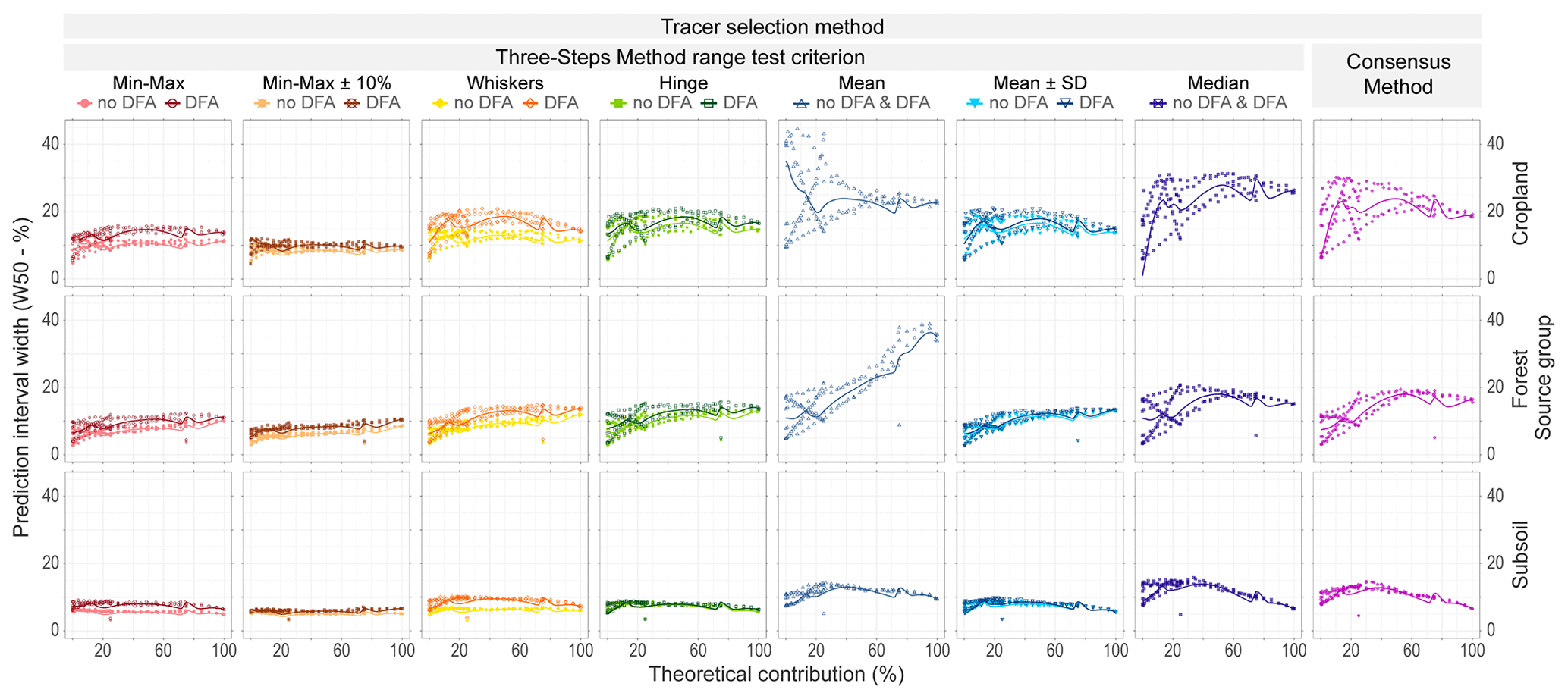
Figure 5 Relationship between theoretical virtual mixture source contributions and prediction interval width (W50) across sources (cropland, forest and subsoil), according to each tracer selection approach: three-step method (TSM) range test criteria, which are minimum–maximum (red circle), minimum–maximum ± 10 % (brown crossed circle), whiskers (yellow/orange diamond), hinge (green square), and mean ± SD (blue triangle point down) – filled and empty symbols correspond to the selection before DFA (no DFA) and after DFA respectively, except for mean (blue triangle) and median (blue crossed square) criteria for which empty symbols correspond to the same selection of tracers before and after DFA – and consensus method (CM; purple circle plus).

Regarding the model residuals for all tracer selections except that obtained with the mean criteria, the error for subsoil was low (RMSE = 6 % to 8 %) with a small bias (ME = −3 % to 5 %). In contrast, forest and cropland errors were about twice higher (RMSE = 10 % to 20 %), with a negative bias for forest (ME = −19 % to −2 %) and a positive bias for cropland (ME = 2 % to 11 %). Accordingly, forest and cropland contributions were underestimation and overpredicted, respectively.

In terms of model performance, the subsoil predictions were highly linear (r² = 0.97–0.99) and well predicted (NSE = 0.92–0.95). For the TSM criteria, linearity and prediction quality were slightly improved in most cases. Nevertheless, a slight decrease in precision and accuracy was observed for contributions below 10 % and above 80 % (Fig. 6). Forest predictions were highly linear for most tracer selections (r² = 0.92–0.98), although their prediction quality was lower (NSE = 0.58–0.86) due to an underestimation (i.e. ME values, Fig. 6). This underestimation was also confirmed by the CRPS values, which increased strongly and linearly above 20 % of forest contribution (Fig. 6). Cropland predictions were relatively linear (r² =  0.71–0.89) but not well predicted (NSE = 0.52–0.80), representing the lowest performance among the sources. The CRPS curves were U-shaped, with a decrease in accuracy and precision for contributions below 60 % and above 70 % (Fig. 7). This pattern was also observed on the observed versus predicted plots in Fig. 6, with a tipping point at around 40 % to 60 % of the contribution. In addition, for a contribution below 60 %, two types of behaviour were observed regardless of the tracer selection method considered (Fig. 6). One group of virtual mixtures was well predicted with a small bias and low CRPS values (≤0.05), while another group was significantly less well predicted with a strong positive bias and higher CRPS values (Fig. 7). These two groups correspond to virtual mixtures with a dominant proportion of subsoil and forest, respectively. For contributions above 60 %, these two groups converge, and no difference can be observed. This suggests that selected tracers were able to successfully discriminate between subsoil and forest sources, while cropland was confused with one of the other two sources.

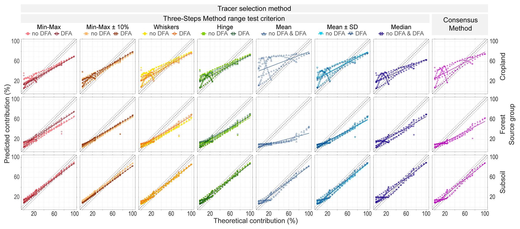
Figure 6 Relationship between theoretical and predicted virtual mixture source contributions (cropland, forest and subsoil), according to each tracer selection approach: three-step method (TSM) range test criteria, which are minimum–maximum (red circle), minimum–maximum ± 10 % (brown crossed circle), whiskers (yellow/orange diamond), hinge (green square), and mean ± SD (blue triangle point down) – filled and empty symbols correspond to the selection before DFA (no DFA) and after DFA respectively, except for mean (blue triangle) and median (blue crossed square) criteria for which empty symbols correspond to the same selection of tracers before and after DFA – and consensus method (CM; purple circle plus).

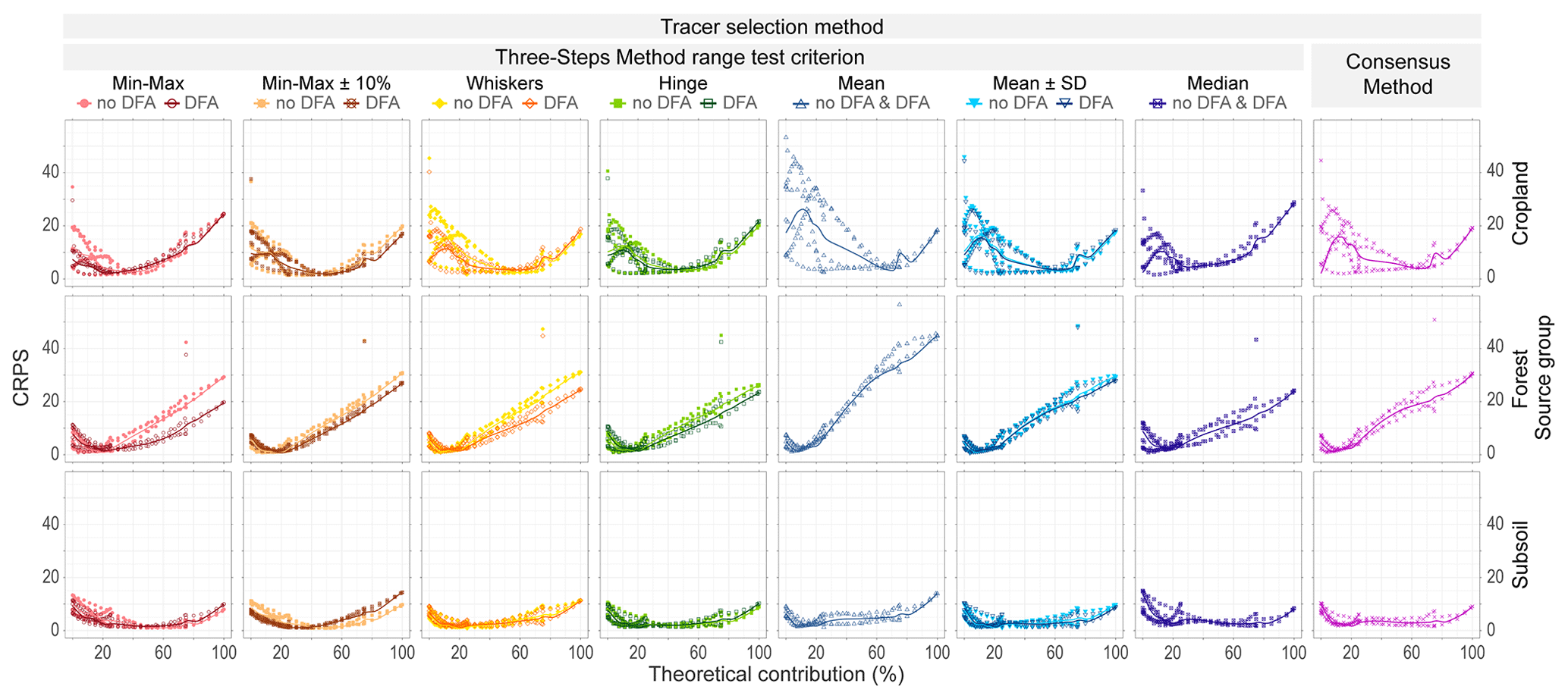
Figure 7 Relationship between theoretical virtual mixture source contributions and continuous ranked probability score (CRPS) across sources: three-step method (TSM) range test criteria, which are minimum–maximum (red circle), minimum–maximum ± 10 % (brown crossed circle), whiskers (yellow/orange diamond), hinge (green square), and mean ± SD (blue triangle point down) – filled and empty symbols correspond to the selection before DFA (no DFA) and after DFA respectively, except for mean (blue triangle) and median (blue crossed square) criteria for which empty symbols correspond to the same selection of tracers before and after DFA – and consensus method (CM; purple circle plus).

Among the selection of tracers, the mean range test criterion was the one that resulted in the lowest prediction quality (Fig. 4). Despite the fact that subsoil had a prediction quality close to that of the other methods, cropland and forest were poorly predicted (NSE = −0.17 and 0.00 respectively), with modelled contributions being quite far from the theoretical values (Figs. 6 and 7).

3.3 Source contribution predictions

The tracer selection methods resulted in three types of source contribution trends: strong dominance of forest, strong dominance of cropland, and equivalent contribution of forest and cropland (Fig. 8).

For all approaches, subsoil contributions were low and stable, for most methods from 0 ± 1 % to 8 ± 3 %. The mean and mean ± SD criteria without DFA led to higher and more variable subsoil contributions than other methods, 12 ± 5 % versus about 4 ± 2 %. The relationship between cropland and forest was different depending on the tracer selection method. For the CM, the mean and median criteria led to model outputs showing that cropland was dominant compared to forest along the sediment core. In contrast, according to the mean ± SD and hinge criteria, the contributions of cropland and forest were modelled to be similar or with only a slight dominance of forest. Finally, for the minimum–maximum, minimum–maximum ± 10% and whiskers criteria, the model calculated a strong dominance of forest over cropland. The DFA had limited impact on the trends in the contributions of cropland and forest for the mean ± SD and hinge criteria, although it resulted in a significant smoothing of the contribution values for the minimum–maximum, minimum–maximum ± 10 % and whiskers criteria. The contribution of cropland was greatly reduced from 16 %–27 % to 2 %–8 % and the dominance of forest increased from 67 %–80 % to 89 %–97 %, resulting in an almost unique and stable contribution from forests along the entire core. However, the contributions of cropland and forest showed similar variations and tendencies along the sediment core for all tracer selection methods, although their values were significantly different. Samples taken at 9/10–10/11, 11/12–13/14, 19/20–20/21 and 24/25–7/28 cm depths were associated with higher contributions from forest and lower contributions from cropland compared to upper/lower samples.

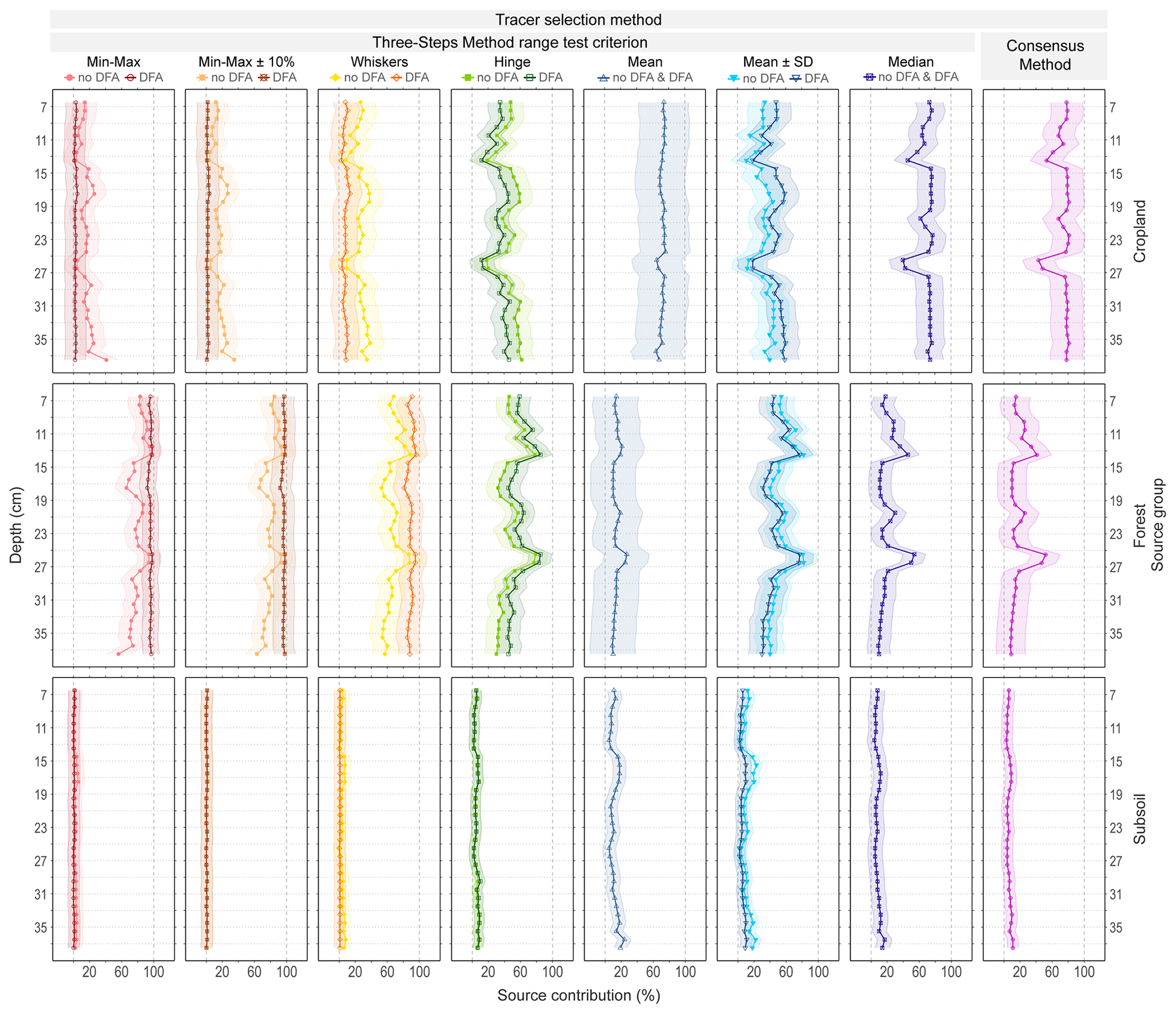
Figure 8 Predicted source contributions for the sediment core samples according to each tracer selection approach. The different range test criteria of the three-step method (TSM) are the following: minimum–maximum (red circle), minimum–maximum ± 10 % (brown crossed circle), whiskers (yellow/orange diamond), hinge (green square), mean (blue triangle), mean ± SD (light blue triangle point down), and median (purple crossed square); the consensus method (CM; light purple circle plus) is also shown. Empty and filled symbols correspond to the use of DFA or not. The error buffer ribbons around the plotted values correspond to the respective RMSE values calculated on virtual mixtures.

The selected tracers did not provide the same information and therefore did not provide the same ability to discriminate between the sources (Fig. 9). For most of the tracers, the following relationship between source group signatures (i.e. mean and SD of log-transformed values) was observed: cropland showed intermediate values, with either forest (TOC, TN) or subsoil (Al, Si, L^*, a^*, b^*, C^*, A2, Q7/4, G₅₂₅) being the highest values. For most of these tracers, cropland had similar values as those of forest (TOC, TN, Si, a^*, b^*, C^*, A2, Q7/4) or subsoil (G₅₂₅). For a few tracers, cropland had the higher values with either subsoil (Zn, Gt) or forest (h) corresponding to the lower values. However, for h, the signatures of cropland and subsoil were similar, and this similarity was also observed for Zn in cropland and forest and for Gt in forest and subsoil sources. In addition, for some selected tracers (Ca, K, Sr, Zr, A1), all source signatures were all very close and hardly distinguishable, making the information derived from the relationships between sources less clear.

Depending on the tracer, sediment sample values did not show the same position in relation to the source signatures (Fig. 9). For some tracers, sample values were close to those of cropland (i.e. Zn, b^*, A1, Q7/4), forest (Al, K, Zr, L^*) or subsoil (a^*, C^*, h). However, for most of the tracers (i.e. TOC, TN, Ca, Si, Sr, A2, Gt, G₅₂₅) sample values were intermediate between those of cropland and forest.

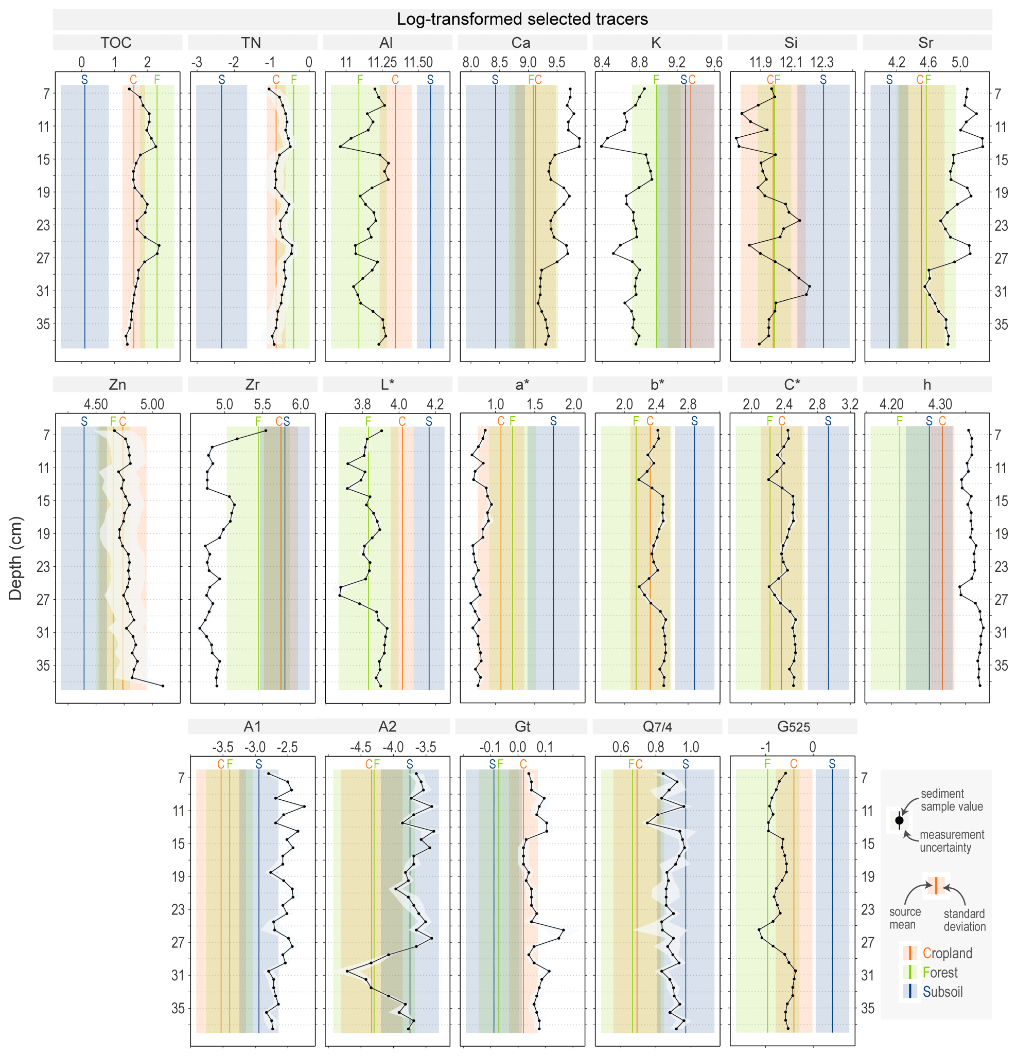
Figure 9 Log-transformed values of selected tracers along the sediment core (black dot; measurement uncertainty is represented with a grey buffer) and in the potential source signatures (vertical line represents mean value, and the buffer zone along each line represents the standard deviation).

4 Discussion

4.1 Conservative behaviour assessment

The different tests used to assess conservative behaviour, i.e. the TSM range test using different criteria and the CM CI, resulted in the selection of properties with different restriction levels. These tests can be divided into three groups according to the number of properties selected, from the least restrictive (minimum–maximum, minimum–maximum ± 10 %, whiskers), via moderately restrictive (hinge, mean ± SD) to the more restrictive (CI, mean, median). Overall, the conservative behaviour tests tended to mainly identify the same properties as being conservative: TOC, TN, b^*, C^* and Q7/4.

In this study, all the tests identified organic matter properties as conservative (i.e. TOC and TN), except for the mean criterion, which did not select TOC. To assess the composition of organic matter, either from terrestrial and/or freshwater origin, the distribution of δ¹³C versus $\mathrm{C}/\mathrm{N}$ ratio can be compared to thresholds (Lamb et al., 2006). In a previous study conducted on a sediment core sampled from the same site in Hayama Lake in 2014, Huon et al. (2018) concluded that there was no autochthonous input of freshwater-originating organic matter, which was confirmed in our data (see Fig. C1 in Appendix C). Organic matter and carbon may be expected to provide a conservative property (García-Comendador et al., 2023), and this is supported by their widespread selection.

Among the geochemical properties, Al, Ti and Si were frequently selected by range tests. This can be explained by their well-known low solubility (Meybeck and Helmer, 1989; Phillips and Greenway, 1998; Koiter et al., 2013) and more specifically for Al and Si, which are constituents of clay sheets given the granitic geological context of the study area (see Fig. B2 in Appendix B). However, these geochemical properties are sensitive to grain size sorting that is occurring along the transport pathway as they are clay sheet constituents. Other geochemical properties that were rarely selected (i.e. Fe, Pb, Ca, K) or systematically rejected, such as Mn, are associated with higher solubility or higher desorption susceptibility (Koiter et al., 2013; García-Comendador et al., 2023; Meybeck and Helmer, 1989; Phillips and Greenway, 1998).

Among the visible colour indices, all conservative behaviour tests selected Q7/4, and other indices such as G₅₂₅, b^*, C^* and L^* were widely selected. The colour indices L^*, b^* and C^* were highly correlated with organic matter properties (i.e. TOC and TN) that were also identified as conservative (Pearson r² from −0.61 to −0.77; see Table A5). This is consistent with the fact that organic matter and iron oxides are the main soil-colouring elements. The existence of different visible-colour spaces provides several tools for sediment fingerprinting studies and for selecting the most appropriate space and indices according to the local context (Viscarra Rossel et al., 2006). These colour spaces are interconnected, and the transformation of indices can be achieved with simple mathematical formula. However, care must be taken to avoid multi-colinearity when using multiple indices from different colour spaces together, as redundancy of information tends to degrade modelling accuracy (Cox et al., 2023). However, the visible-colour parameters are quite sensitive to spatial and temporal variations (García-Comendador et al., 2023). The acquisition of other spectral regions such as Vis–NIR, NIR (near-infrared) and MIR (mid-infrared) appears to be more robust (Chen et al., 2023), especially as these regions are a powerful and reliable way to obtain the extensive range of properties and information on the sample with the advantages of being rapid, cost-effective and non-destructive measurements (Soriano-Disla et al., 2014). Of note is that in order to ensure the exchange of spectra within the community, the adoption of a common protocol and/or the provision of calibration spectra using inter-calibration samples should be discussed, as spectra tend to be instrument-dependent (Pimstein et al., 2011).

The CI was a restrictive method compared to most range test criteria. It selected four properties, which is similar to the number of properties selected by the mean and median range test criteria. Nevertheless, some properties selected by other range test criteria, which were a priori conservative properties, showed a score close to the threshold of 0.00 defined by Lizaga et al. (2020). Thus, Al, Si, Ti, Q7/4 and G₅₂₅ obtained a CI equal to −0.1, while it was equal to −0.2 for Zn, L^* and A2. This could indicate that properties that yielded a CI score close to the threshold (i.e. 0.00) were not strictly conservative (e.g. size sorting for Al, Si and Ti). We suggest that either the CI can be used to identify less conservative properties in a selection resulting from different tests or from the modification of the CI threshold (i.e. not strictly equal to 0.00) to select properties currently considered not conservative.

As this study shows, a priori and field knowledge are essential to assess the relevance of conservative behaviour assessments (Laceby et al., 2015; Koiter et al., 2018; Batista et al., 2019). However, this knowledge is not sufficient and not usable for all measured properties, especially for relatively new properties as colour parameters, due to their complex relationship with environmental processes. Other studies developed particle size and organic matter corrections, which were shown to be effective (Koiter et al., 2018). However, they require additional measurements and are site-specific (Koiter et al., 2018). Therefore, it is essential to develop cost-effective, time-effective and generalised methods (Koiter et al., 2018).

4.2 Tracer selection and contribution modelling

The CR index was designed to select properties based on their relevance to prediction, as they maximise convergence. Of the 24 properties considered in the current research, only the TOC, TN, b^*, L^* and G₅₂₅ reached a CR score above 70 (Fig. 3). These properties were redundant, as they showed very similar trends along the sediment core (Fig. 9). By removing tracers that prevent consensus, CR favours redundant properties and discards dissenting properties that could nevertheless be relevant, and this may lead to an information gap. Dissenting properties can provide complementary information, as properties do not discriminate between sources in the same way.

Indeed, the selection of consistent properties can result in the prediction of a dominant source while ignoring another. For example, in this study, the CR selected properties for which sediment values were close to the cropland signature or were intermediate between cropland and forest values (Fig. 9). This selection of tracers with consistent cropland signature resulted in the prediction of dominant cropland contributions (Fig. 8).

Conversely, the DFA stepwise procedure of the TSM aims to maximise the difference between properties by simultaneously minimising redundant information, which could increase the prediction quality of MixSIAR (Cox et al., 2023). In this study, the use of the DFA improved model accuracy for all the range test criteria compared to the selection prior DFA (Fig. 4). However, DFA application tended to reduce source contribution variations – especially for minimum–maximum, minimum–maximum ± 10% and whiskers criteria – (Fig. 8). Overall, the impact of the DFA on tracer selection modelling outputs needs more research to be clarified.

From the different tracer selections, which were all distinct, three main tendencies were observed in terms of modelled contributions (Fig. 8). On the one hand, extensive tracer selections, such as minimum–maximum, minimum–maximum ± 10 % and whiskers criteria, resulted in a modelled dominance of the forest contribution over cropland and subsoil. On the other hand, restrictive selections of tracers, such as the CM, mean and median criteria, resulted in a modelled dominance of cropland contribution. Finally, methods that selected an intermediate number of tracers, i.e. mean ± SD and median criteria, led to the prediction of a balanced contribution between forest and cropland. This major impact of the tracer selection methods on the source contribution modelling was demonstrated by multiple studies (Laceby et al., 2015; Palazón et al., 2015; Smith et al., 2018; Gaspar et al., 2019).

However, in the current research, all methods agreed on a low subsoil contribution associated with high modelling accuracy statistics (Fig. 4). It can be assumed that since all tracer selection methods selected TN, b^* and C^*, they allowed us to predict the general trend of the subsoil contribution behaviour. Thus, methods that selected additional tracers, such as mean ± SD and median criteria, did not result in significant modifications of the trend. However, the methods that selected a large number of tracers (i.e. minimum–maximum, minimum–maximum ± 10 % and whiskers) resulted in a strong reduction or even disappearance of the subsoil contribution, on average about 2 % versus 8 %. The need for few tracers to predict subsoil with a good prediction accuracy can be explained by its significantly different signature compared to forest and cropland (Fig. 9). Most of the modelling limitations were related to the prediction quality for cropland and forest, as their respective signatures were very close to each other for many tracers (Fig. 9). However, the same variations, i.e. higher forest and lower cropland contributions, were observed for most methods. These variations could be explained by the information provided through the incorporation of TN and TOC contents, which were the most frequently selected tracers. That is consistent with the results of Huon et al. (2018), which associated a higher TOC content with a high forest contribution. Furthermore, for the methods that selected Al, these contribution variations were sharper and more detailed, especially for samples collected from the upper part of the sediment core (i.e. depth from 7 to 17 cm).

Of note, additional metrics, such as sensitivity analysis or variable importance approach, could provide a more detailed understanding of the role of each tracer in contribution predictions (Russi et al., 2008; Bennett et al., 2013; Wei et al., 2015).

4.3 Assessing modelling prediction accuracy

The generation of virtual mixtures allowed for the evaluation of model prediction accuracy for a wide range of source contributions. The use of several metrics allowed us to describe different aspects of the modelling (i.e. residuals, accuracy and precision) and to better interpret the prediction on real sediment samples (Latorre et al., 2021; Batista et al., 2022). The graphical representation of the metrics (Figs. 5, 6, and 7) allowed us to identify ranges of source contributions with different prediction accuracies. This understanding of the model supports a better appreciation and interpretation of predictions on sediment samples.

Virtual mixtures were generated to cover the full range of potential combinations of source contributions, varying from 0 % to 100 % with 5 % increments. The range of predicted contributions for virtual mixtures (i.e. minimum and maximum) defines the space of possible model predictions obtained with a given set of tracers. However, for the majority of the tracer selections investigated here, part or totality of the sediment sample predicted contributions fell outside of the space of the virtual mixture predicted contributions (Table A6). This result may be explained by the fact that the assumptions made when generating virtual mixtures were not respected. For instance, tracers may not behave fully conservatively during erosion processes (Koiter et al., 2013) or a source may not have been correctly identified or classified (Palazón et al., 2015; Smith et al., 2018; Batista et al., 2022). Novel techniques should be developed to quantify the extent to which a property is modified during transport (i.e. depletion or enrichment) (García-Comendador et al., 2023) to support the generation of virtual mixtures with tracer values that better represent the reality. Here, virtual mixtures were generated as simple proportional mixtures of mean properties of each source tracer, which implies that all properties are considered strictly conservative properties. This has likely not been fully achieved with the commonly implemented tests (i.e. range tests and CI). Indeed, the use of not fully conservative tracers may result in the generation of virtual mixture property values that differ from those observed in actual sediment samples. This may raise concerns regarding the validity of modelling prediction accuracy statistics calculated with virtual mixtures and their direct transferability to actual sediment samples. Accordingly, we may hypothesise that the farther the sediment sample predicted contributions are from the space of virtual mixture predicted contributions, the less transferable the accuracy statistics of the model will be to actual sediment samples. In our opinion this comparison may help with appreciating the level of confidence in the metrics calculated using virtual mixtures and their direct transferability to the model predictions obtained for actual sediment samples. This may lead to over-interpretation or misinterpretation. Future research could usefully develop novel metrics to quantify this level of confidence and better support model evaluation.

5 Conclusions

In this study, we compared two source sediment fingerprinting tracer selection methods, the TSM and the CM, for their selection of tracers and their resulting predictions of source contributions for a single dataset. Conservative behaviour tests of both methods were compared, including a total of seven different TSM range test criteria and the CM CI. The different tests resulted in different selections of properties that had different sensitivity levels. On the one hand, the minimum–maximum, minimum–maximum ± 10 % and whiskers range test criteria selected a large number of properties, from 12 to 23 out of 24 potential properties, including non-conservative properties. On the other hand, the mean and median criteria and the CI selected a low number of properties, from 3 to 4 tracers, which can lead to limitations when modelling source contributions in target samples. The mean ± SD and hinge criteria resulted in an intermediate selection of tracers, selecting from 7 to 9 properties. Although differences were observed among methods, some tracers were selected by most of the methods (i.e. TOC, TN, b^*, C^* and Q7/4), showing some consistency among them. Although the different methods resulted in different selections of tracers, three main contribution tendencies were observed in relation with the number of tracers selected. Indeed, methods that selected a large number of tracers resulted in a strong dominance of forest. In contrast, a limited selection of tracers resulted in a dominant contribution of cropland. Finally, balanced contributions of forest and cropland were obtained for the methods selecting an intermediate number of tracers. Based on this high variability of selected tracers among methods, future research should develop novel metrics to quantify and qualify the conservative behaviour of tracer properties during erosion and transport processes.

To assess modelling accuracy, 138 virtual mixtures were generated as a simple proportional mixtures of sources individual properties. Several modelling accuracy metrics were computed for each tracer selection using virtual mixture predicted contributions. These metrics and their associated representations provided a useful support to better evaluate the impact of each tracer selection method on model predictions. However, for most of the tracer selections, a strong divergence in the range of predicted contributions was observed for virtual mixtures and those values obtained for actual sediment samples. These divergences highlight the fact that evaluation metrics obtained for virtual mixtures are likely not directly transferable to prediction obtained for actual sediment samples. Metrics should be used with caution, to avoid over-interpretation or misinterpretation of modelling results. These divergences may likely be attributed to the selection of tracer properties with a not (fully) conservative behaviour during erosion, transport and deposition processes, which could not be quantified and reproduced when generating the virtual mixtures with currently available methods. New methods should be designed to generate virtual mixtures closer to reality to better evaluate modelling accuracy.

Among the compared methods, the high variability of selected tracers among the TSM and the CM, and within the TSM according to the range test criteria, was associated with strong divergences on modelling output results. This may raise concerns regarding the use of quantitative outputs as it may not meet the ultimate goal sought for by fingerprinting approaches as they are currently implemented by the scientific community. Consequently, to avoid a potential loss of confidence of stakeholders regarding the validity of the outputs of this method in the future, it is essential to take as much care as possible to conduct an accurate and reliable identification of conservative behaviour, as the whole methodology and the results rely on this initial step. This is fundamental both for improving our understanding of erosion and sedimentation processes and for guiding the implementation of effective landscape management measures. Accordingly, we encourage our colleagues from the scientific community to share their tracing datasets obtained in contrasted environmental conditions around the world in order to contribute to the further improvement, development and evaluation of sediment source fingerprinting techniques.

Appendix A

A1 Statistics

Table A1 Summary of MixSIAR accuracy statistics calculated on virtual mixtures (n = 138) for each tracer selection method: three-step method (TSM) range test criteria and consensus method (CM) for cropland course. W50^*: prediction interval width; ME: mean error; RMSE: root mean square error; r²: squared Pearson's correlation coefficient; NSE: Nash–Sutcliffe modelling efficiency coefficient; CRPS: continuous ranked probability score. Note that ^* indicates mean values per source.

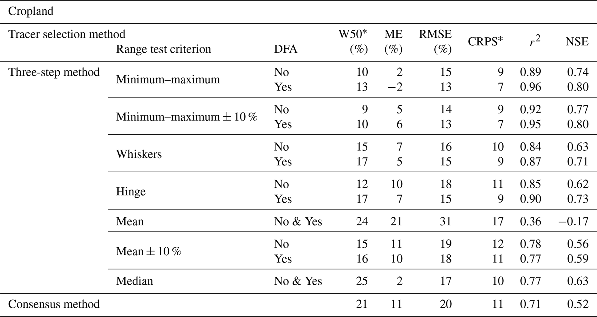
Table A2 Summary of MixSIAR accuracy statistics calculated on virtual mixtures (n = 138) for each tracer selection method: three-step method (TSM) range test criteria and consensus method (CM) for forest course. W50*: prediction interval width; ME: mean error; RMSE: root mean square error; r²: squared Pearson's correlation coefficient; NSE: Nash–Sutcliffe modelling efficiency coefficient; CRPS: continuous ranked probability score. Note that ^* indicates mean values per source.

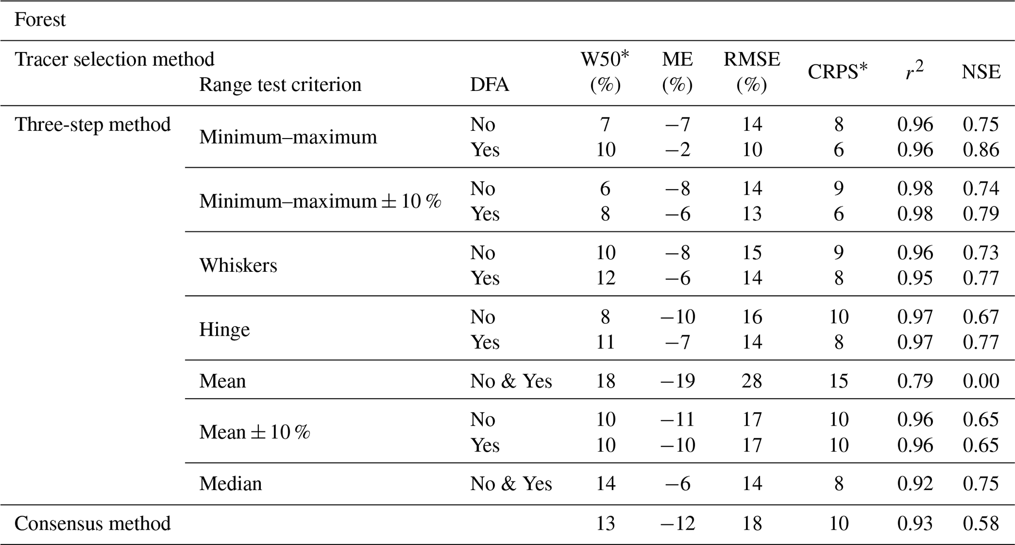
Table A3 Summary of MixSIAR accuracy statistics calculated on virtual mixtures (n = 138) for each tracer selection method: three-step method (TSM) range test criteria and consensus method (CM) for subsoil course. W50^*: prediction interval width; ME: mean error; RMSE: root mean square error; r²: squared Pearson's correlation coefficient; NSE: Nash–Sutcliffe modelling efficiency coefficient; CRPS: continuous ranked probability score. Note that ^* indicates mean values per source.

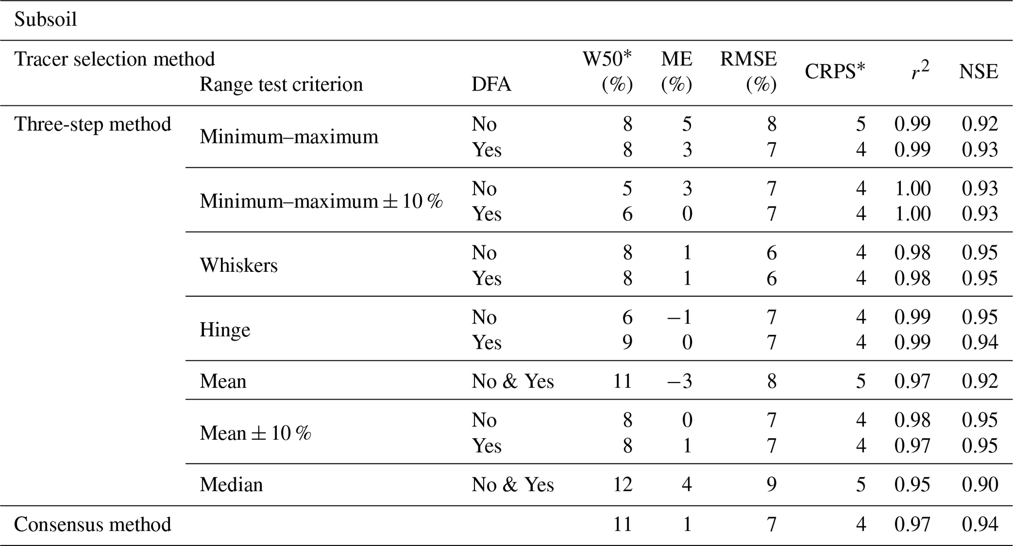
Table A4 Summary of MixSIAR accuracy statistics calculated on virtual mixtures (n = 138) for each tracer selection method: three-step method (TSM) range test criteria and consensus method (CM) averaged on the three sources (i.e. cropland, forest and subsoil). W50^*: prediction interval width; ME: mean error; RMSE: root mean square error; r²: squared Pearson's correlation coefficient; NSE: Nash–Sutcliffe modelling efficiency coefficient; CRPS: continuous ranked probability score. Note that ^* indicates mean values per source.

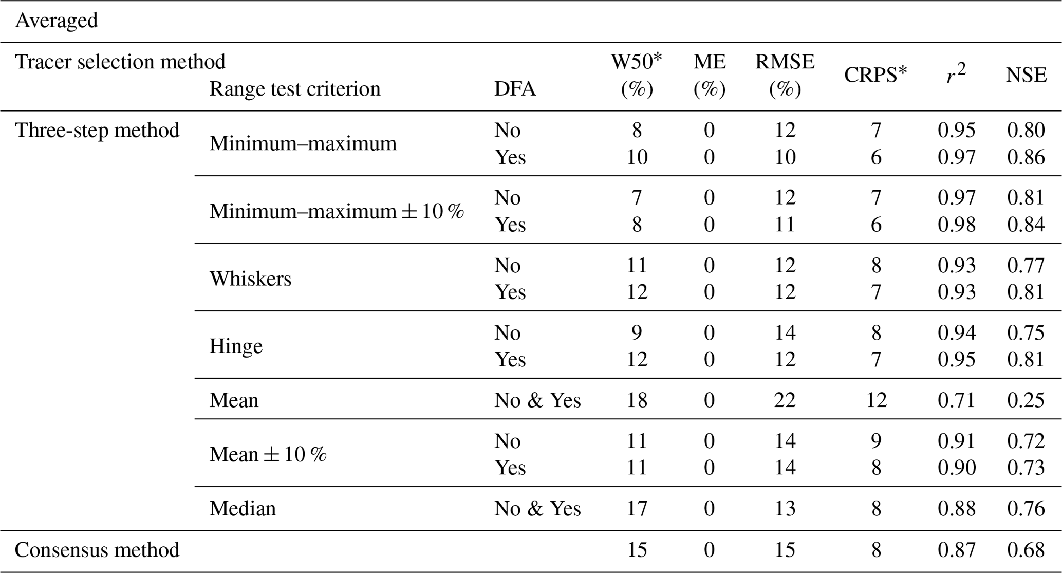
Table A5 Selected tracer Pearson correlation coefficients. The symbol ⋅ represents correlation with significance test p value lower than 0.05.

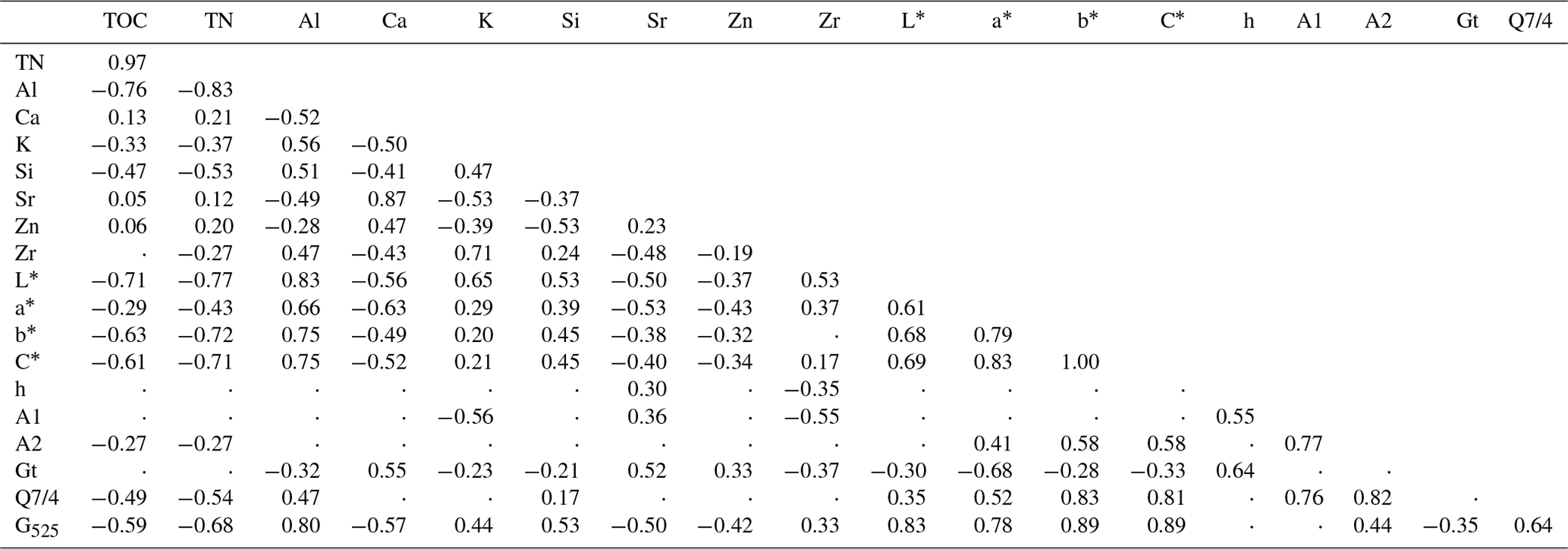
Table A6 Number of sediment samples that fell inside of the space of the virtual mixture predicted contributions for each tracer selection method out of 32.

Appendix B: Maps

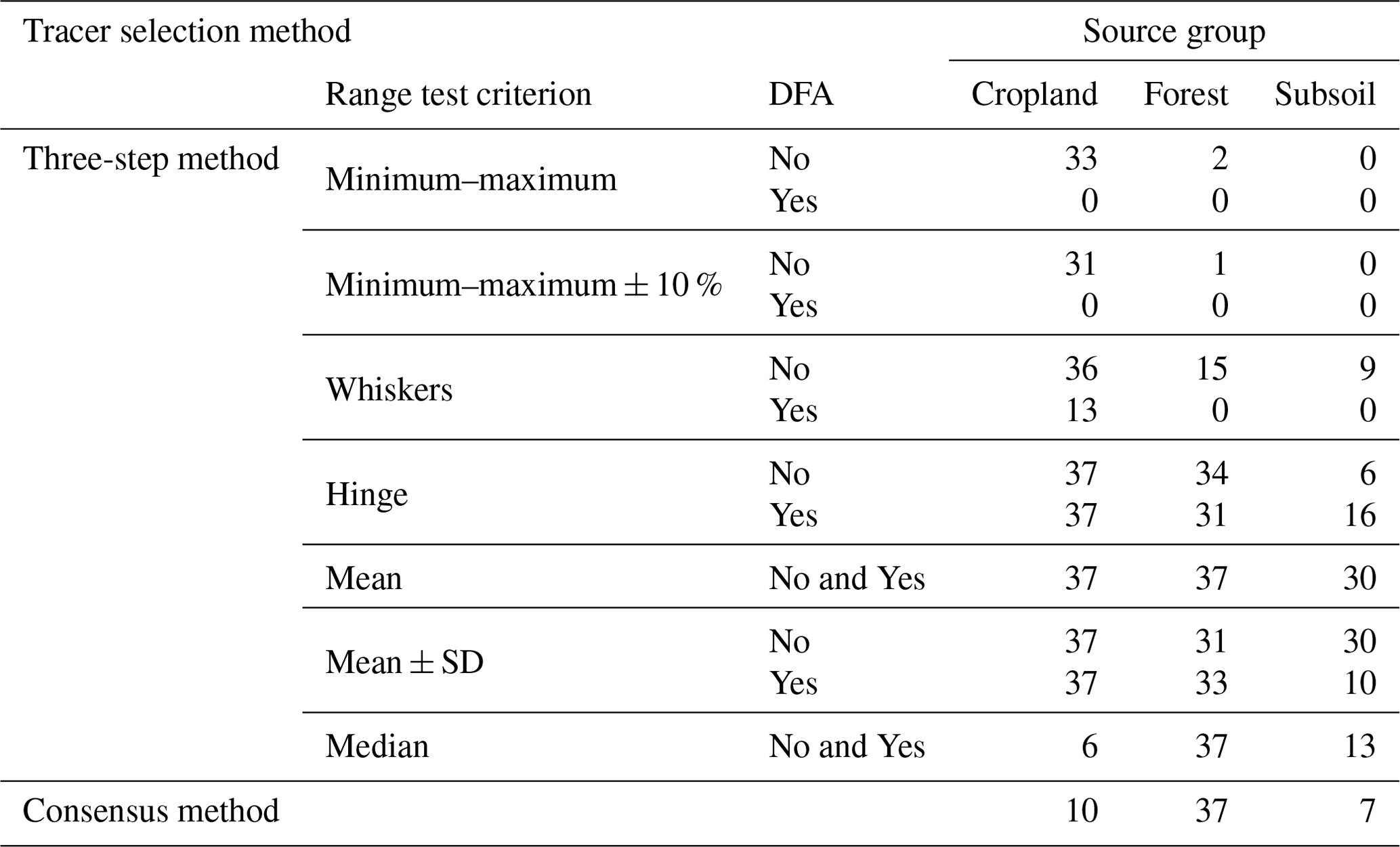
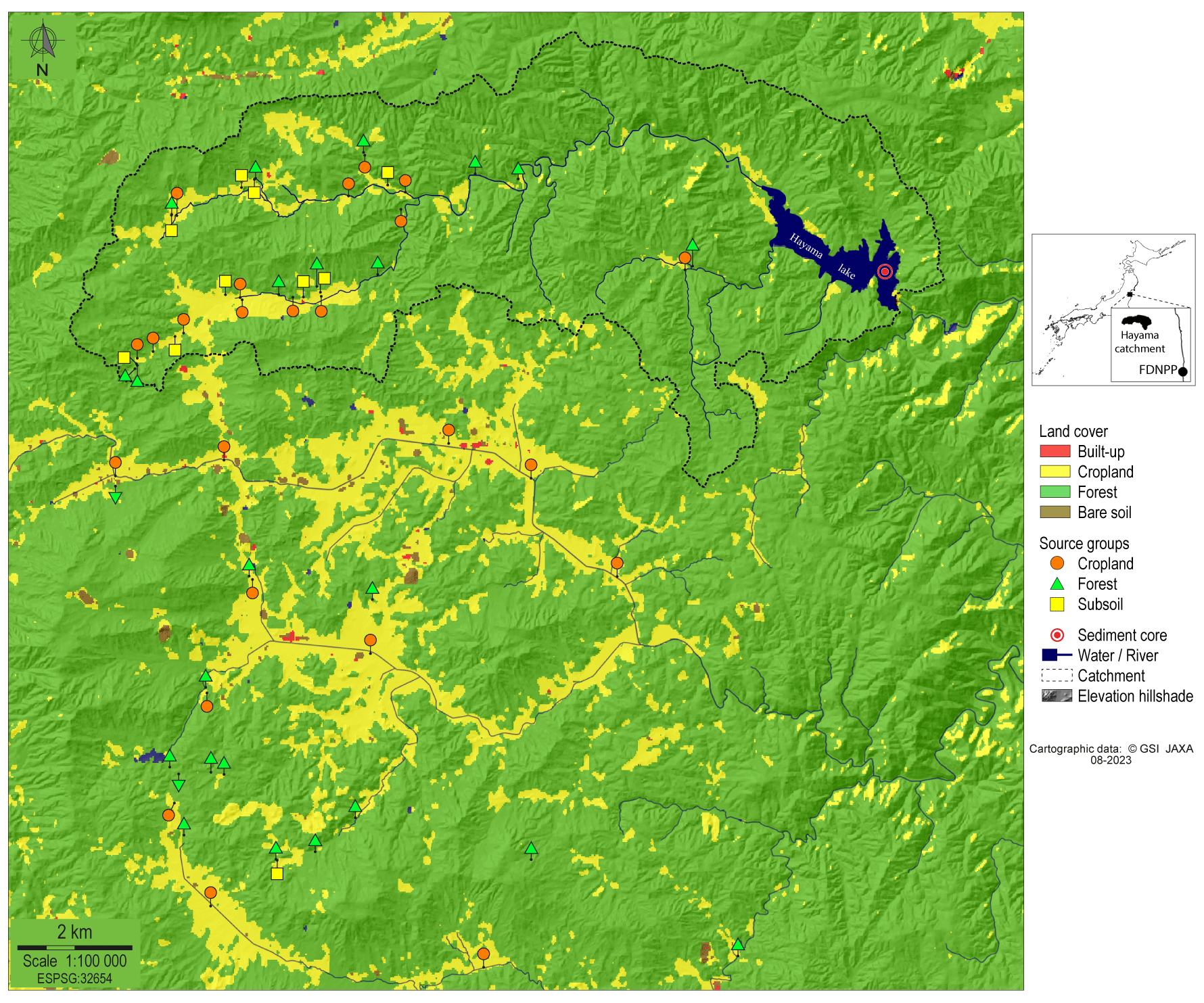
Figure B1 Map of the main land uses in the study area over the 2014–2016 period with location of the source samples and the sediment core (cartographic data: GSI and JAXA). FDNPP: Fukushima Daiichi Nuclear Power Plant.

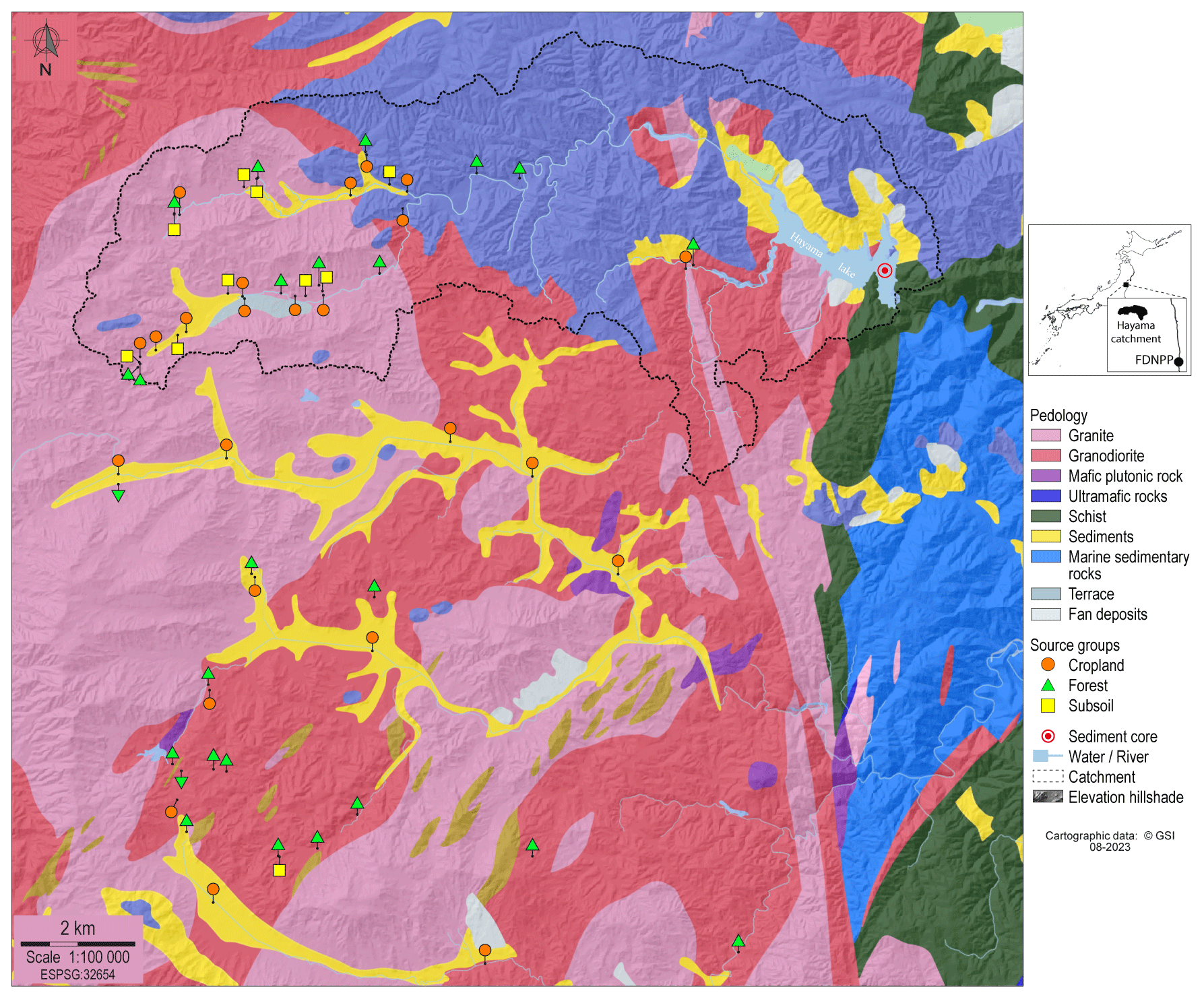
Figure B2 Map of the main geology types in the study area with location of the source samples and the sediment core (cartographic data: GSI). FDNPP: Fukushima Daiichi Nuclear Power Plant.

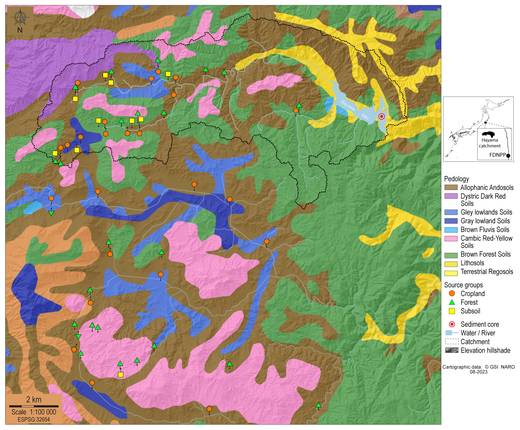
Figure B3 Map of the main soil types in the study area with location of the source samples and the sediment core (cartographic data: GSI and NARO). FDNPP: Fukushima Daiichi Nuclear Power Plant.

Appendix C: Laboratory analysis

C1 Organic matter

In the Hayama Lake catchment, sediment and soils were found to not contain carbonate minerals, and all the carbon associated with particulate matter is organic in nature (Huon et al., 2018). Total organic carbon (TOC) and total nitrogen (TN) elemental concentrations and isotopes (δ¹³C and δ¹⁵N) were determined by combustion using a continuous-flow elementary analyser (Elementar Vario PYRO cube) coupled with an isotope ratio mass spectrometer (EA-IRMS) (Micromass Isoprime) at the Institute of Ecology and Environmental Sciences (iEES, Paris) in France. A first analysis was conducted to measure TOC concentrations together with a set of tyrosine standards (Coplen et al., 1983). The second analysis was dedicated to measure TN concentrations after sample weight optimisation from TOC results. For combustion, oxygen was injected during 70 s (30 mL min⁻¹) at 850 ^∘C for reduction, and the combustion furnace was at 1120 ^∘C (Agnihotri et al., 2014). The analytical precision was assessed with repeated analyses of a tyrosine internal standard (n = 51), calibrated against international reference standards (Girardin and Mariotti, 1991). The analysis of these properties in source material is described in detail in the study by Laceby et al. (2016b). To evaluate whether the samples are composed of terrestrial or freshwater-originating material, the distribution of sample values was plotted in a δ¹³C versus TOC/TN diagram and compared to the thresholds reported in Lamb et al. (2006) (Fig. C1).

C2 Geochemistry

Elemental geochemistry was determined using X-ray fluorescence (XRF) (Malvern Panalytical, ED-XRF Epsilon 4). A total of 17 elemental concentrations were measured (Al, Ca, Co, Cr, Cu, Fe, K, Mg, Mn, Ni, Pb, Rb, Si, Sr, Ti, Zn, and Zr). Measurements were conducted in containers covered with a 3.6 µm thin Mylar film (Chemplex, Mylar thin-film cat. no. 157) with a 10 mm exposure surface. A minimum of 0.1 g of material was analysed. To consider the potential heterogeneity within a sample, three replicate measurements were made, and the mean value of these replicates was calculated. To assess the accuracy of the measurements, a standard (JMS-1, sediment from the Tokyo Bay, Terashima et al., 2002) was measured every seven samples (n = 38), and the accuracy of the measured batch was determined based on the calculation of the root mean square errors (RMSE).

C3 Visible colorimetry

Visible colorimetry was measured using a portable diffuse reflectance spectrophotometer, Konica Minolta CM-700d, set on a 3 mm target radius. Samples were measured in a plastic zip bag. In order to account for potential heterogeneities within a sample, three measurements were made at different locations on the bag. The spectrophotometer was calibrated at the start of each set of measurements with a zero (black) and white standards. Measurements were conducted according to the D65 illuminance standard, 10^∘ angle observer and excluding the specular component. The spectral reflectance (in %) was measured from 360 to 740 nm with a 10 nm resolution (30 wavelength classes). Raw data were processed using the colour data software CM-S100w SpectraMagic NX (Konica Minolta, 2022). Colour parameters within the Cartesian coordinate systems CIE Lab (1976) (i.e. L^*, a^* and b^*) (CIE, 2008) and CIE LCh (i.e. C^* and h) were exported. The CIE LCh is a vector representation of the CIE Lab (1976). C and h are derived from a^* and b^* parameters. Within the CIE Lab system, L^* is the lightness of the colour, from black (0) to white (100); a^* is the position between green to red (negative values are associated with green and positives with red); and b^* is the position between blue and yellow (negative values are associated with blue and positive values with yellow). Within the CIE LCh system, C^* is the chroma (positive values are associated to brighter colours and negative values to duller colours), and h is the hue angle (in ^∘) in the CIE Lab colour wheel.

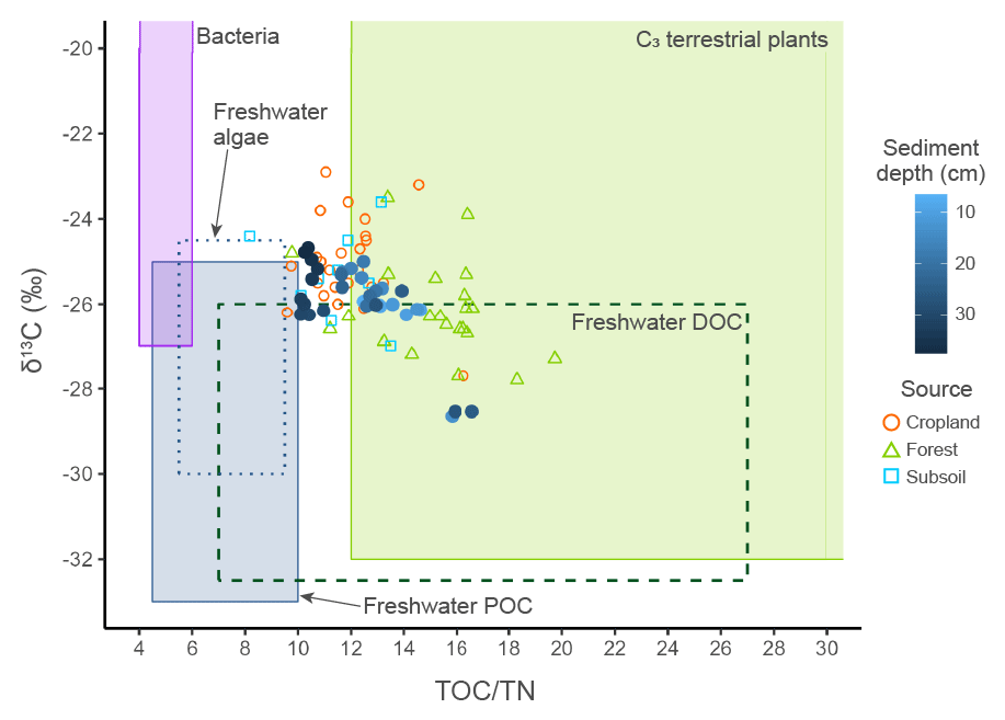
Figure C1 Sediment core and source samples δ¹³C and TOC/N and typical ranges for organic inputs to lacustrine environments (thresholds from Lamb et al., 2006).

The Q7/4 ratio as defined by Debret et al. (2011) was calculated as the ratio between 700 and 400 nm reflectance values. This ratio provides a numerical description of the reflectance spectrum general slope.

The oxy-hydroxide geothite (α-FeOOH) soil richness can be determined using visible diffuse reflectance spectra (Kosmas et al., 1984; Balsam et al., 2004; Hao et al., 2009; Torrent et al., 2007), and its peak values at 445 and 525 nm were calculated from the first derivative reflectance spectrum (Debret et al., 2011). In our case, the geothite concentration was not aimed for, only the relative abundance among our samples in order to differentiate between them. For each replicate of the measurements and for each sample, the first derivative reflectance spectrum was calculated and smoothed with a Savitzky–Golay filter using the savitzkyGolay function (differentiation order = 1, polynomial order = 3, window size = 5 (equivalent to 50 nm)) from R package prospectr (Stevens and Ramirez-Lopez, 2022) (Wadoux et al., 2021). Then the mean per sample and the standard deviation were calculated. From the first derivative of reflectance, two geothite peaks were calculated: first, the 445 nm peak value was calculated as the mean of values at 440 and 450 nm, and second, the 525 nm peak was calculated as the mean of those at 520 and 530 nm (Debret et al., 2011).

The remission function was calculated from the reflectance spectrum: f(R) = (1−R)² according to the Kubelka–Munk relationship (Scheinost et al., 1998). Then, the second derivative was calculated and the spectrum was smoothed with a Savitzky–Golay filter using the savitzkyGolay function (differentiation order = 2, polynomial order = 3, window size = 5). From the second derivative of the remission function spectrum, the iron oxide-associated parameters (A1, A2, A3) and the goethite proportion within iron oxides (Gt) were obtained (Tiecher et al., 2015). The A1 and A2 peaks are associated with goethite, and the A3 peak is associated with hematite; all peaks were calculated as the amplitude between each maximum and minimum band. Thus, A1 is the difference between 450 and 420 nm, A2 is the difference between 510 and 480 nm, A3 is the difference between 575 (as the mean of 570 and 580 nm) and 535 nm (as the mean of 530 and 540 nm), and Gt is calculated as the ratio of $\mathrm{A}\mathrm{1}/(\mathrm{A}\mathrm{1}+\mathrm{A}\mathrm{3})$.