Does soil thinning change soil erodibility? An exploration of long-term erosion feedback systems

Soil erosion rates on arable land frequently exceed the pace at which new soil is formed. This imbalance leads to soil thinning (i.e. truncation), whereby subsoil horizons and their underlying parent material become progressively closer to the land surface. As soil erosion is a selective process and subsurface horizons often have contrasting properties to the original topsoil, truncation-induced changes to soil properties might affect erosion rates and runoff formation through a soil erosion feedback system. However, the potential interactions between soil erosion and soil truncation are poorly understood due to a lack of empirical data and the neglection of long-term erodibility dynamics in erosion simulation models. Here, we present a novel model-based exploration of the soil erosion feedback system over a period of 500 years using measured soil properties from a diversified database of 265 agricultural soil profiles in the UK. For this, we adapted the Modified Morgan–Morgan–Finney model (MMMF) to perform a modelling experiment in which topography, climate, land cover, and crop management parameters were held constant throughout the simulation period. As selective soil erosion processes removed topsoil layers, the model gradually mixed subsurface soil horizons into a 0.2 m plough layer and updated soil properties using mass-balance mixing models. Further, we estimated the uncertainty in model simulations with a forward error assessment. We found that modelled erosion rates in 99 % of the soil profiles were sensitive to truncation-induced changes in soil properties. The soil losses in all except one of the truncation-sensitive profiles displayed a decelerating trend, which depicted an exponential decay in erosion rates over the simulation period. This was largely explained by decreasing silt contents in the soil surface due to selective removal of this more erodible particle size fraction and the presence of clayey or sandy substrata. Moreover, the soil profiles displayed an increased residual stone cover, which armoured the land surface and reduced soil detachment. Contrastingly, the soils with siltier subsurface horizons continuously replenished the plough layer with readily erodible material, which prevented the decline of soil loss rates over time. Although our results are limited by the edaphoclimatic conditions represented in our data, as by our modelling assumptions, we have demonstrated how modelled soil losses can be sensitive to erosion-induced changes in soil properties. These findings are likely to affect how we calculate soil lifespans and make long-term projections of land degradation.

1 Introduction

Rates of soil erosion on agricultural land often exceed the rates at which new soil is formed (Evans et al., 2019; Montgomery, 2007). This imbalance is one which, left unchecked, can pose a critical threat to the sustainability of global soil resources and their ability to deliver vital ecosystem services across environments and society (Bot et al., 2000; Quinton et al., 2010). Moreover, as soils become thinner (i.e. truncated), the subsoil horizons and their underlying parent material become progressively closer to the land surface. This process might affect physical, chemical, and biological topsoil properties (Bouchoms et al., 2019; Papiernik et al., 2009; Vanacker et al., 2019), as well as soil water availability to plants and ultimately crop growth (Herbrich et al., 2018; Öttl et al., 2021; Schneider et al., 2021).

For instance, plot- and catena-based studies report that truncated agricultural soil profiles often display increased clay and/or sand contents in their Ap horizons (Rhoton and Tyler, 1990), compared to the soils from non-eroding positions in the landscape. Moreover, eroded Ap horizons tend to have higher bulk density, lower organic carbon content, and lower water holding capacity (Olson and Nizeyimana, 1988; Stone et al., 1985; Strauss and Klaghofer, 2001). However, such patterns are highly variable and greatly dependent on the properties of the underlying subsoil material being progressively tilled into the Ap horizon (Lowery et al., 1995).

Erosion-induced changes to soil depth and soil properties can therefore influence soil losses and runoff formation through a soil erosion feedback system (Morgan et al., 1984; Vanwalleghem et al., 2017). That is, erosion-induced changes to soil physical properties might affect soil erodibility (i.e. the susceptibility of soil to erosion), which may accelerate or slow down soil losses. Understanding how such a system might develop over time and under assorted conditions is an important step to proactively design and implement effective soil conservation strategies, as different soils are likely to be impacted by erosion in varied ways (Hoag, 1998). However, the empirical data over decadal to centennial timescales required to explore the feedbacks between soil erosion and soil thinning are currently non-existent. It follows that process-oriented soil erosion models are arguably the only available tool to simulate how erosion processes interact with truncation-induced changes in the soil system.

Process-oriented models allow for a representation of multiple mechanisms that influence soil erosion, from basic processes such as particle detachment by raindrop impact and surface runoff, to more complex interactions between soil properties, hydrological processes, climate, and plant cover (see Merritt et al., 2003 for an overview). This ability to simulate the response of specific soil erosion processes to external stimuli makes process-oriented models useful for exploring what-if scenarios. Hence, models such as the Water Erosion Prediction Project (WEPP; Nearing et al., 1989), the LImburg Soil Erosion Model (LISEM; De Roo et al., 1996), and the Morgan–Morgan–Finney model (MMF; Morgan, 2001; Morgan et al., 1984; Morgan and Duzant, 2008) have been used to explore the impacts of land use or climate change on soil erosion (e.g. Anache et al., 2018; Eekhout et al., 2021; Nearing et al., 2005).

To date, most soil erosion models and model users assume that the inherent erodibility of different soil horizons down a soil profile is constant over the period of a model simulation. As upper soil horizons are removed by erosion, thereby exposing the subsurface material, the implicit assumption in soil erosion modelling is that this erodibility is not variable, such that any changes to projected erosion rates are solely a factor of climate, land cover, and topography (e.g. Ciampalini et al., 2020; Eekhout et al., 2021; Panagos et al., 2021). However, since erodibility is a reflection of soil physical, chemical, and biological properties, and given that subsoils typically (although not exclusively) exhibit contrasting soil properties to those observed in upper horizons, it follows that erodibility is not necessarily a constant as a soil profile thins. Furthermore, soil erodibility might change over longer timescales due to the coarsening and armouring of surface soils (Sharmeen and Willgoose, 2007; Willgoose and Sharmeen, 2006) and the depletion of erodible material as a result of extreme soil truncation (Anselmetti et al., 2007).

Although the soil erosion feedback system has been recognised as a key challenge for modelling past and future erosion rates (Vanwalleghem et al., 2017), long-term dynamics of soil erodibility are an underexplored topic in erosion research. Exceptions come from landscape evolution models which simulate the influence of erosion and deposition on soil development over millennia (van der Meij et al., 2020; Sommer et al., 2008). However, in areas under severe erosion rates, subsoil horizons can be exposed within a matter of decades (Evans et al., 2020), which might trigger unexpected responses regarding runoff formation and soil losses. Moreover, soil truncation can introduce substantial spatial variability to soil properties, often not accounted for in static soil maps used for a variety of purposes (Świtoniak et al., 2016). Still, the lack of knowledge about the potential interactions between soil erosion and soil erodibility (i.e. in which timescale are erosion feedback mechanisms developed, how are different soil properties and soil types affected by truncation?) interpose the representation of soil truncation in the applications of soil erosion models.

Here, we hypothesise that erosion-induced changes to soil properties affect soil loss rates over long-term periods. To evaluate such a hypothesis, we performed an exploration of the soil erosion feedback system by simulating 500 years of soil losses and surface runoff on 265 agricultural soil profiles in the UK. This allowed us to investigate how soil erosion rates respond to truncation-induced changes in soil properties and unravel the processes potentially driving such responses in different soil types in the UK. To the best of our knowledge, this is the first time soil erosion models have been used to understand the interactions between soil erosion, soil thinning, and soil erodibility, and how these interactions are established in varying soil types. An enhanced understanding of such a dynamic soil erosion feedback system will be crucial for improving the calculation of soil lifespans, providing future soil loss projections, and designing long-term soil conservation strategies.

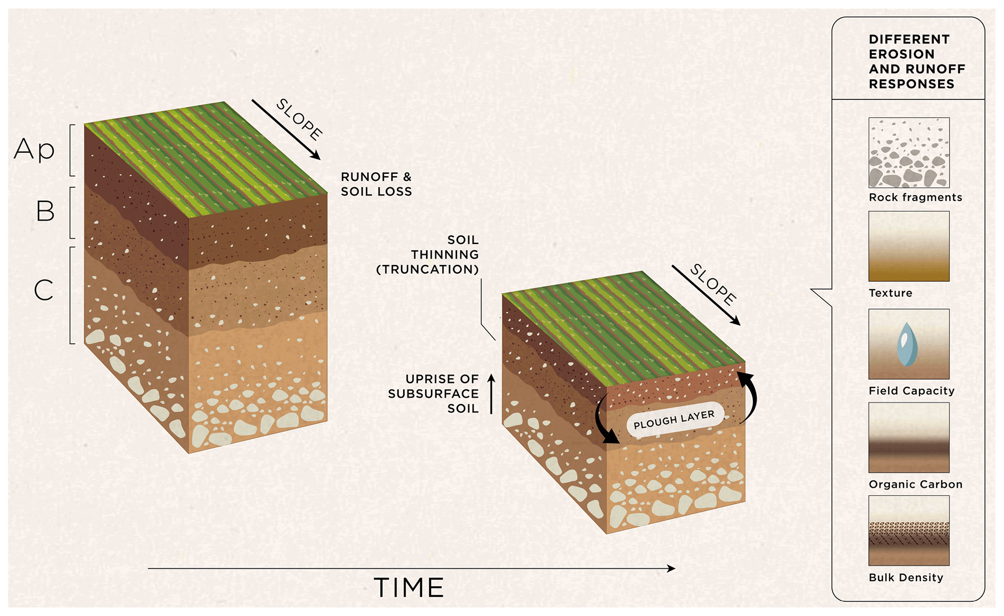
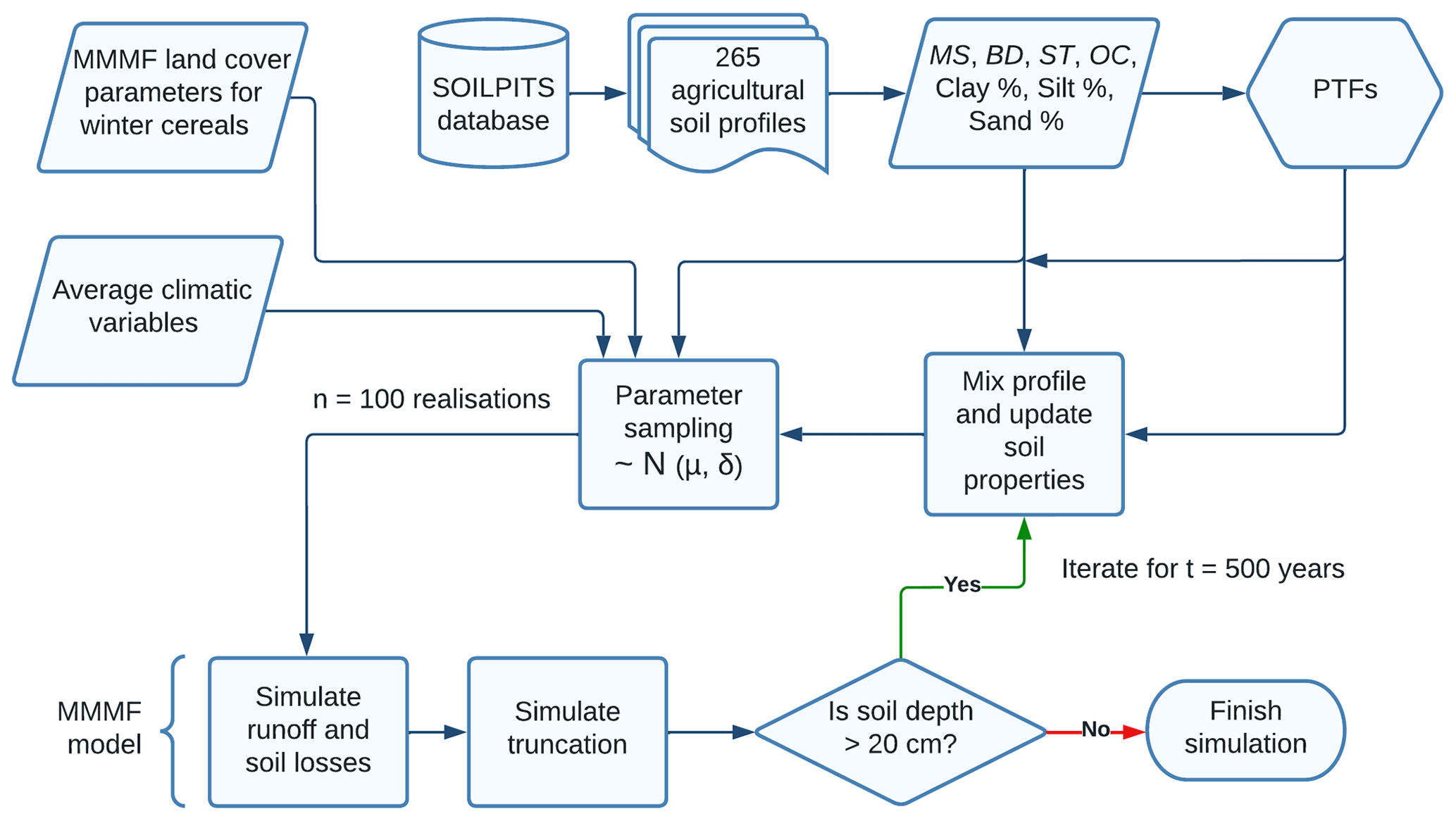
Figure 1 Modelling concept: selective soil erosion processes alter topsoil properties, which are then mixed with the underlying substrata as the soil profile thins. Updated soil properties for the plough layer are used as model inputs for the following time step.

2 Materials and methods

2.1 Concept

Our modelling concept is essentially a numerical thought experiment, in which land cover, agricultural management, climate, and topography parameters are held within a constant range, so that any changes in simulated soil losses and surface runoff over a period of 500 years are solely a result of changes in soil properties due to erosion processes (Fig. 1). To perform this experiment, we parameterised a soil erosion model using measured data from 265 agricultural soil profiles spread across the UK (Fig. 2). The abstract spatial scale of the simulations can be perceived as a pedon located on a conventionally tilled hillslope with winter cereals. For simplicity, we assume this spatial unit does not receive runoff and sediment input from upslope. As the original topsoil of each profile/pedon is successively removed by erosion, our model gradually mixes the subsurface horizons into a 0.2 m plough layer (i.e. the average tillage depth in the UK, Townsend et al., 2016), continuously updating soil properties through mass-balance models and pedotransfer functions (PTFs, Fig. 1).

In order to implement our modelling concept, we adapted the Modified Morgan–Morgan–Finney (MMMF) model (Morgan and Duzant, 2008). The model was chosen due to its ability to simulate multiple erosion subprocesses, which is desirable for understanding the specific mechanisms responsible for developing erosion feedback systems. That is, MMMF represents particle size selectivity during erosion, transport, and deposition, incorporates the effects of stone cover on soil detachability, and simulates particle detachment by both raindrop impact and surface runoff. In addition, the MMMF model has a parsimonious parameter set, which facilitates model application using national soil survey datasets. Moreover, MMMF and its derivatives have provided acceptable predictions of annual soil losses for different soils, land covers, and testing sites in the UK (Morgan and Duzant, 2008; Peñuela et al., 2018; Smith et al., 2018). In the following section we provide a brief description of the basic MMMF equations (Sect. 2.2). We subsequently characterise the soil profile database used for the modelling (Sect. 2.3) and describe the model implementation, including the mixing of surface and subsurface horizons (Sect. 2.4).

2.2 MMMF operating equations

The MMMF is a process-oriented conceptual model running on an annual time step, in which soil erosion processes are separated into a water phase and a sediment phase (Morgan et al., 1984; Morgan and Duzant, 2008). In the water phase, effective annual rainfall (P_EF; mm) is calculated considering the effect of interception by the vegetation cover:

$$\begin{array}{}\text{(1)}& P_{\text{EF}}=P\cdot (\mathrm{1}-\text{PI}),\end{array}$$

where P is the mean annual rainfall (mm) and PI is the average rainfall interception (proportion 0–1) afforded by the vegetation cover. For annual crops, PI and all other land cover parameters are taken as an approximate average over the growing season.

Annual leaf drainage (LD; mm) and direct throughfall (DT; mm) are separated as a function of the average canopy cover of the vegetation (CC; proportion 0–1):

$$\begin{array}{}\text{(2)}& {\displaystyle }\text{LD}=P_{\text{EF}}\cdot \text{CC},\text{(3)}& {\displaystyle }\text{DT}=P_{\text{EF}}-\text{LD}.\end{array}$$

The kinetic energy of direct throughfall KE_DT is calculated with the typical value of erosive rainfall intensity for a given location (I; mm h⁻¹) and the amount of annual direct throughfall, whereas the kinetic energy of leaf drainage KE_LD is a function of the average plant height for the growing season (PH; m) and the amount of the annual leaf drainage. Total kinetic energy of the effective annual rainfall (KE; J m⁻²) is then calculated as the sum of the throughfall and leaf drainage components:

$$\begin{array}{}\text{(4)}& {\displaystyle }{\text{KE}}_{\text{DT}}=\text{DT}\cdot (\mathrm{8.95}+\mathrm{8.44}\cdot {\text{log}}_{\mathrm{10}}I),\text{(5)}& {\displaystyle }\text{if}\text{PH}<\mathrm{0.15};{\text{KE}}_{\text{LD}}=\mathrm{0},\text{(6)}& {\displaystyle }\text{if}\text{PH}\ge \mathrm{0.15};{\text{KE}}_{\text{LD}}=\text{LD}\cdot (\mathrm{15.8}\cdot {\text{PH}}^{\mathrm{0.5}}-\mathrm{5.87}),\text{(7)}& {\displaystyle }\text{KE}={\text{KE}}_{\text{DT}}+{\text{KE}}_{\text{LD}}.\end{array}$$

Of note is that in the original MMMF publication (Morgan and Duzant, 2008), as well as in the revised Morgan–Morgan–Finney paper (Morgan, 2001), Eq. (6) does not include the LD parameter. However, this would lead to the KE_LD being expressed in J mm⁻¹ m⁻² instead of J m⁻². Hence, we highlight that a correct application of Eq. (6) must include leaf drainage depth (see Brandt, 1990; Morgan et al., 1998; Peñuela et al., 2018).

Saturation-excess overland flow typically occurs in climates with low intensity precipitation and without a pronounced seasonal rainfall regime (Morgan and Duzant, 2008), specifically in areas with shallow soils and impermeable bedrocks (Beven, 2012). In the MMMF model, generation of saturation-excess runoff is assumed to occur when the mean daily rainfall exceeds the mean daily storage capacity of the soil (SC; mm):

$$\begin{array}{}\text{(8)}& \text{SC}=\mathrm{1000}\cdot \text{MS}\cdot \text{BD}\cdot \text{HD}\cdot {\left({\displaystyle \frac{{\text{ET}}_{\text{a}}}{{\text{ET}}_{\text{p}}}}\right)}^{\mathrm{0.5}},\end{array}$$

where MS is soil moisture at field capacity (% w w⁻¹), BD is bulk density (Mg m⁻³), HD is effective hydrological depth (m) (i.e. the land-cover-dependent soil depth in which storage capacity controls the generation of runoff), and ET_a / ET_p is the ratio of actual to potential evapotranspiration. These parameters represent an approximate average for the cropping season.

The annual runoff generation (Q; mm) is then estimated as a function of annual effective rainfall, the ratio between storage capacity and mean daily rainfall (P_M, mm), and the slope length of the spatial modelling element (L; m):

$$\begin{array}{}\text{(9)}& Q=P_{\text{EF}}\cdot e^{\left(-\frac{\text{SC}}{P_{\text{M}}}\right)}\cdot {\left({\displaystyle \frac{L}{\mathrm{10}}}\right)}^{\mathrm{0.1}}.\end{array}$$

In the sediment phase, the annual detachment of soil particles by raindrop impact (E_R; kg m⁻²) and by surface runoff (E_Q; kg m⁻²) are calculated separately for the clay, silt, and sand texture classes, which are subsequently summed as follows:

$$\begin{array}{}\text{(10)}& {\displaystyle }{E}_{\text{R}}=\sum _{n=\mathrm{1}}^i\left[K_{{\text{R}}_i}\cdot {\displaystyle \frac{T_i}{\mathrm{100}}}\cdot \left(\mathrm{1}-\text{ST}\right)\cdot \text{KE}\cdot {\mathrm{10}}^{-\mathrm{3}}\right],\text{(11)}& {\displaystyle }{E}_{\text{Q}}=\sum _{n=\mathrm{1}}^i\left\{K_{{\mathrm{Q}}_{\mathrm{i}}}\cdot {\displaystyle \frac{T_i}{\mathrm{100}}}\cdot Q^{\mathrm{1.5}}\cdot \left[\mathrm{1}-\left(\text{GC}+\text{ST}\right)\right]\cdot {\text{sin}}^{\mathrm{0.3}}\cdot S\cdot {\mathrm{10}}^{-\mathrm{3}}\right\},\end{array}$$

where K_R is the detachability of the soil by raindrop impact (J m⁻²), T is the percentage of texture class i, ST is stone cover (proportion 0–1), K_Q is the detachability of the soil by runoff (J m⁻²), GC is the average proportion of the soil covered by vegetation during the growing season (0–1), and S is slope angle (degrees). Soil detachability values for each texture class i (clay, silt, and sand) are taken from Quansah (1982).

The immediate deposition of detached sediments (D; %) (i.e. the percentage of sediments not delivered to the runoff for transport) is estimated as a function of the average annual flow velocity, in our case for vegetated conditions (v_v; m s⁻¹), and the particle fall number (FN):

$$\begin{array}{}\text{(12)}& {\displaystyle }{v}_{\text{v}}={\left({\displaystyle \frac{\mathrm{2}\cdot g}{\mathit{ø}\cdot \text{NV}}}\right)}^{\mathrm{0.5}}\cdot S^{\mathrm{0.5}},\text{(13)}& {\displaystyle }{\text{FN}}_i={\displaystyle \frac{L\cdot v_{{\text{s}}_i}}{v_{\text{v}}\cdot d}},\text{(14)}& {\displaystyle }{D}_i=\mathrm{44.1}\cdot ({\text{FN}}_i{)}^{\mathrm{0.29}},\end{array}$$

where g is the gravitational acceleration (9.81 m s⁻²), ø is the diameter of plant stems (m), NV is the number of stems per unit area (number m⁻²), v_s is the fall velocity for texture class i (0.00002, 0.002 and 0.02 m s⁻¹ for clay, silt, and sand, respectively), and d is the hydraulic radius of the flow (0.005 m for unchannelled flow, 0.01 m for shallow rills, and 0.25 m for deeper rills). Again, in this case, land cover parameter values describe an average over the cropping season.

The total detached material delivered annually to transport (G; kg m⁻²) is modelled separately for each soil texture class i:

$$\begin{array}{}\text{(15)}& G=\sum _{n=\mathrm{1}}^i\left[\left(E_{{\text{R}}_i}+E_{{\text{Q}}_i}\right)\cdot \left(\mathrm{1}-{\displaystyle \frac{D_i}{\mathrm{100}}}\right)\right].\end{array}$$

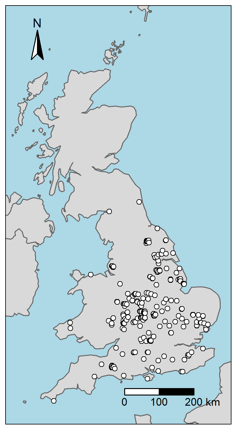
Figure 2 Location of the 265 soil profiles used in this study. Data source: Land Information System (LandIS) (LandIS, 2022).

The annual transport capacity of the surface runoff (TC; kg m⁻²) is calculated as a function of annual runoff volume (Q; mm), slope, and the effect of plant cover/tillage on flow velocities, for each particle size class i:

$$\begin{array}{}\text{(16)}& \text{TC}=\sum _{n=\mathrm{1}}^i\left[\left({\displaystyle \frac{v_{\text{a}}\cdot v_{\text{v}}\cdot v_{\text{t}}}{v_{\text{b}}}}\right)\cdot \left({\displaystyle \frac{T_i}{\mathrm{100}}}\right)\cdot Q^{\mathrm{2}}\cdot \sin S\cdot {\mathrm{10}}^{-\mathrm{3}}\right].\end{array}$$

The average flow velocities for the actual soil conditions (v_a; m s⁻¹), for the effect of tillage (v_t; m s⁻¹), and for the standard bare soil condition (v_b; m s⁻¹) are calculated using the Manning equation:

$$\begin{array}{}\text{(17)}& {\displaystyle }{v}_{\text{a}}={\displaystyle \frac{\mathrm{1}}{n}}\cdot d^{\mathrm{0.67}}\cdot S^{\mathrm{0.5}}\cdot e^{-\mathrm{0.018}\text{ST}},\text{(18)}& {\displaystyle }{v}_{\text{b}};v_{\text{t}}={\displaystyle \frac{\mathrm{1}}{n}}\cdot d^{\mathrm{0.67}}\cdot S^{\mathrm{0.5}},\end{array}$$

where n is Manning's roughness coefficient. For the tilled conditions, Manning's n is estimated as a function of an implement-dependent surface roughness parameter (RFR) taken from Morgan (2005):

$$\begin{array}{}\text{(19)}& n=e^{(-\mathrm{2.11}+\mathrm{0.03}\text{RFR})}.\end{array}$$

The annual soil loss (SL; kg m⁻²) is calculated by comparing the annual transport capacity (TC; kg m⁻²) and the annual sediment delivered to the runoff (G; kg m⁻²) for each texture class i:

$$\begin{array}{}\text{(20)}& \text{If}{\text{TC}}_i\ge G_i;\text{SL}=G_i.\end{array}$$

If the amount of sediment delivered to the runoff is greater than the transport capacity, the excess sediment will be deposited until G=TC. Such deposition is modelled using the settling velocities and fall numbers described in Eq. (14). The sediment balance becomes

$$\begin{array}{}\text{(21)}& \begin{array}{rl}& \text{If}{\text{TC}}_i<G_i\text{calculate}{\text{G1}}_i=G_i\left[\mathrm{1}-\left({\displaystyle \frac{D_i}{\mathrm{100}}}\right)\right],\\ & \mathrm{\text{If}}{\text{TC}}_i\ge {\text{G1}}_i;{\text{SL}}_i={\text{TC}}_i;\text{if}{\text{TC}}_i<{\text{G1}}_i;{\text{SL}}_i={\text{G1}}_i.\end{array}\end{array}$$

Finally, the soil losses for the clay, silt, and sand texture classes are summed to produce total estimates of annual soil losses (SL; kg m⁻²):

$$\begin{array}{}\text{(22)}& \text{SL}=\sum _{n=\mathrm{1}}^i{\text{SL}}_i.\end{array}$$

2.3 Soil database

The soil profile data used in the model were retrieved from the UK SOILPITS dataset, which is one of many datasets held within the Land Information System (LandIS) operated by the Soil and Agrifood Institute at Cranfield University, UK (LandIS, 2022). The UK SOILPITS dataset represents a compilation of a series of soil profile surveys conducted across the UK since 1984. We only selected the profiles under agricultural land cover and those that had complete information on the key soil properties used for modelling.

Table 1 presents a descriptive summary of the data representing each whole soil profile; that is, data for each horizon from each profile has been bulked together. The profiles range in thickness from 0.22 to 1.96 m (median depth is 0.60 m) and are typically composed by four characteristic horizons: an A, E, B, and C horizon. More information about how each horizon was surveyed and differentiated in the field can be found in Hodgson (1997).

Table 1 Descriptive statistics of the soil properties from the 265 agricultural soil profiles (depths between 0.22 and 1.96 m) from the LandIS database used in the simulations.

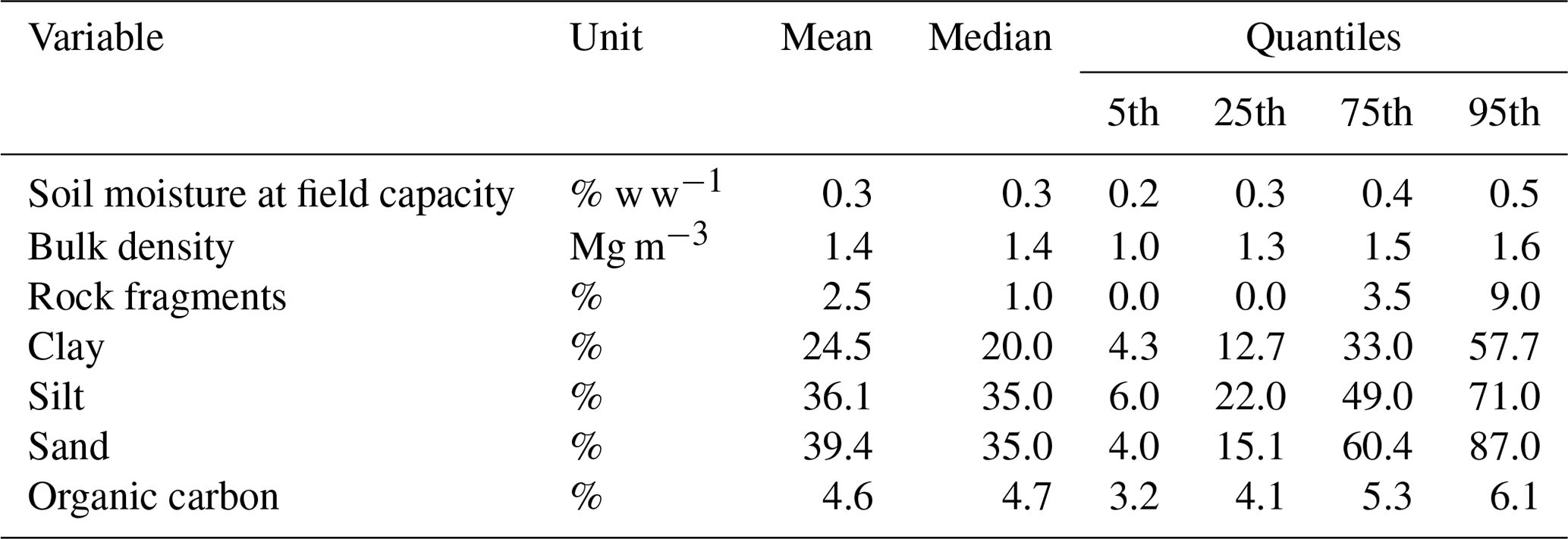
Figure 3 demonstrates the variability of key soil properties within the four characteristic soil horizons, compiling all soil profiles used in the dataset (by “key”, we mean those properties which are employed directly or indirectly as input variables in our model). There is considerable overlap between each horizon, largely due to the heterogeneity of soil types represented in the dataset. However, some distinctive patterns can be discerned. For example, between the A and B horizon, bulk density tends to increase, while organic carbon tends to decrease. Some 79 profiles were also observed to have an E horizon directly below the A horizon. This was distinguished by the presence of a mineral layer with less organic carbon and clay content than the underlying B horizon, indicating downward and/or lateral translocation into the subsoil. Another notable boundary lies between the B and C horizon, where the median soil moisture at field capacity reduces by more than 2.5 times. This may be reflective of some distinctive textural changes between these two horizons: the median sand content increases 3 times, while both clay and silt decrease by more than 5 times.

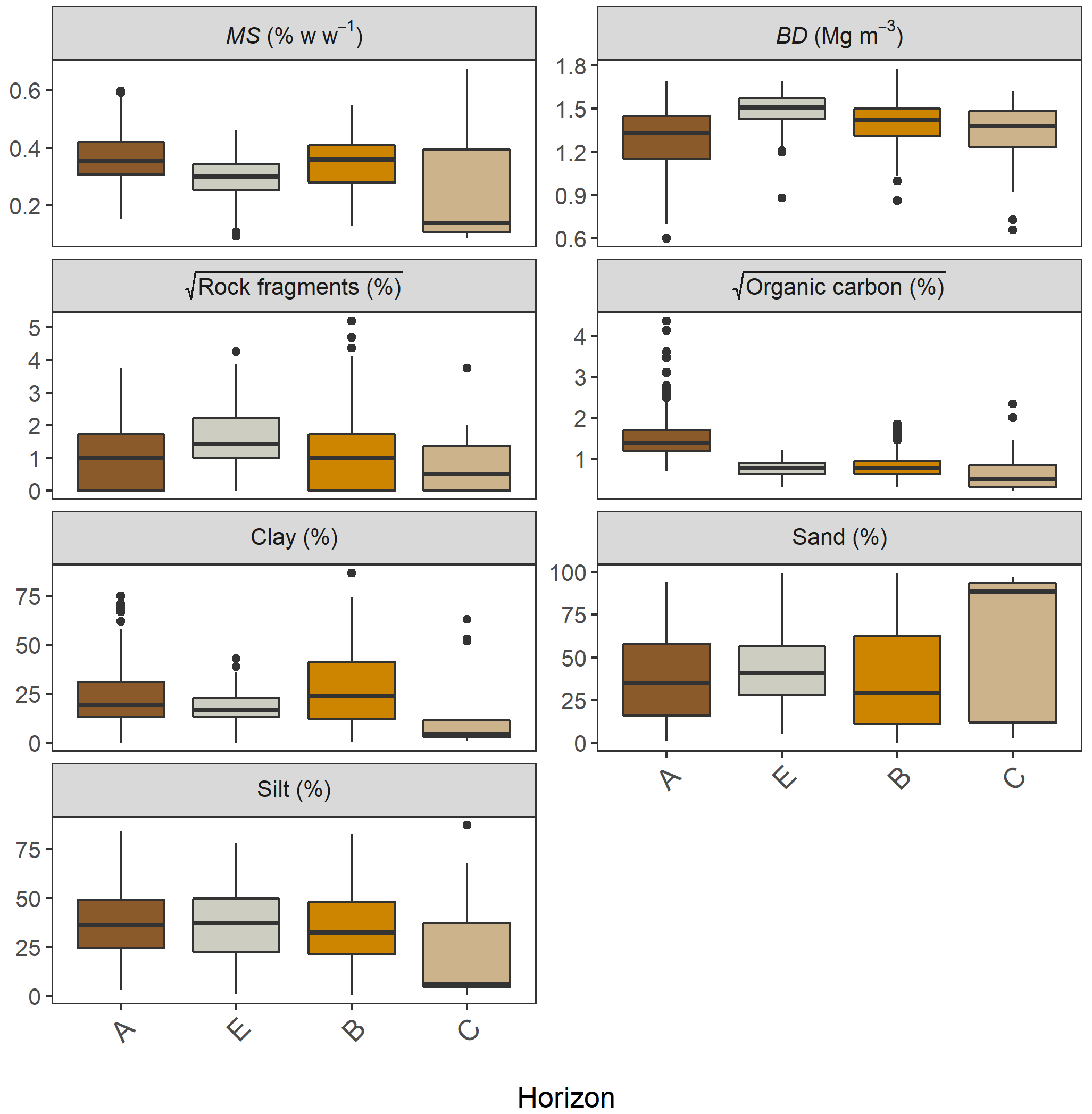
Figure 3 Boxplots of the key soil properties for each horizon of the soil profiles used in this study. Horizons which were not classified, or which occurred less than 5 times in the dataset are not shown in the figure. Organic carbon and rock fragment values underwent a square root transformation to improve the visualisation of the data.

2.4 Model implementation

Our modelling framework consists of an application of the MMMF model for each of the 265 soil profiles over a period of 500 years (Fig. 4). Whilst the variability of the soil properties across profiles and horizons was incorporated into the model, all modelling units were parameterised the same for their climatic, land cover, and topographic variables. This was performed to test the sensitivity of modelled soil losses to erosion-induced changes to soil properties in different soil types.

Figure 4 Flowchart of the modelling framework.

We selected rainfall-associated parameter values based on UK average climatic variables for the 1991–2020 period (Kendon et al., 2021). For the land cover parameters, which represent an approximate average over the crop growing season, we took the guide values recommended by Morgan and Duzant (2008) for conventionally tilled winter cereals, except for plant height (PH) and ground cover (GC). This is because we found that the suggested value of 1.5 m was excessive for winter cereals, especially considering that PH in Eq. (6) does not represent the height of the top of the canopy, but rather the height of the fall of drops from the plant, which depends on the thickness of the canopy (Brandt, 1990). Assuming an average absolute height of 0.61 m for wheat varieties in the UK (Berry et al., 2015), we adopted a baseline PH value of 0.4 m. This was also performed to constrain disproportionate estimates of leaf drainage kinetic energy, as trial model runs indicated a high sensitivity of the model outputs to parameter PH. Moreover, GC was calculated using the number of plants per unit area (NV) and the average diameter of plant elements at ground surface (ø; m), in order to avoid inconsistencies between sampled GC values and the remaining plant parameters.

In addition, we assumed a 10 m slope length and 6^∘ slope gradient for the spatial element of the simulation unit. For the soil parameters, we used the measured properties from the soil profile database (Table 1). Texture-dependent parameter values were taken from the model guide, considering the soils' particle size distribution. A Monte Carlo simulation with 100 iterations per year was included to provide a forward error assessment of the model outputs (Beven, 2009). Model parameters were sampled from a normal distribution with a 10 % standard deviation to partially account for measurement errors and the uncertainty in parameter estimation. The constant parameter distributions used in all simulations are displayed in Table 2.

Table 2 Parameter values which were applied to all soil profiles and sampled in the Monte Carlo simulation.

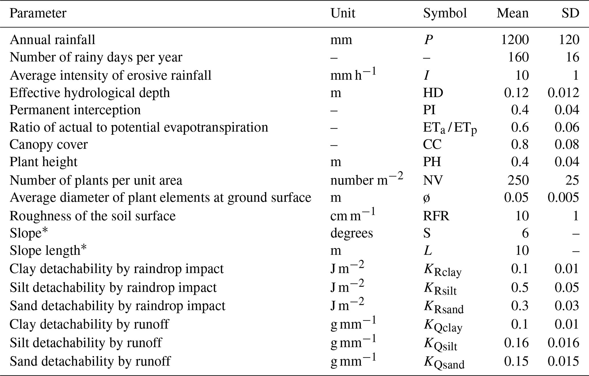
^∗ The parameter value was held constant during the Monte Carlo simulation.

In order to simulate soil thinning, the soil losses (SL; kg m² yr⁻¹) estimated with the MMMF model were converted into SL_m (m yr⁻¹) using soil bulk density (BD; Mg m⁻³):

$$\begin{array}{}\text{(23)}& {\text{SL}}_{\text{m}}={\displaystyle \frac{\text{SL}}{\text{BD}}}\cdot {\mathrm{10}}^{-\mathrm{3}}.\end{array}$$

Next, the model reduced the depth of the upmost soil horizon based on the amount of eroded soil in the previous time step.

The soil texture of the 0.2 m plough layer was updated after each time step k using a mass-balance model considering the amount of fresh subsoil being incorporated into the plough layer and the selective removal of different particle- size fractions. This requires estimating the mass of the original plough layer p in time step k (M_p; kg m⁻²) and the mass of the subsoil layer that will be incorporated by tillage in time step k+1 (M_s; kg m⁻²):

$$\begin{array}{}\text{(24)}& {\displaystyle }{M}_{\text{p}}=\mathrm{0.2}\cdot {\text{BD}}_{\text{p}}\cdot {\mathrm{10}}^{\mathrm{3}},\text{(25)}& {\displaystyle }{M}_{\text{s}}={\text{SL}}_{\text{m}}\cdot {\text{BD}}_{\text{s}}\cdot {\mathrm{10}}^{\mathrm{3}},\end{array}$$

where BD_p is the bulk density (Mg m⁻³) of the original plough layer in time step k and BD_s is the bulk density (Mg m⁻³) of the subsoil layer s being incorporated by tillage in time step k+1. Please note that the estimation of BD for each time step is described in detail below.

The masses of each particle size fraction i in the plough layer for time step k, after selective removal ($M_{{\text{p}}_i}$; kg m⁻²), and in the subsoil layer being incorporated ($M_{{\text{s}}_i}$; kg m⁻²) are then calculated as

$$\begin{array}{}\text{(26)}& {\displaystyle }{M}_{{\text{p}}_i}=\left(M_{\text{p}}\cdot {\displaystyle \frac{T_{i_{\text{p}}}}{\mathrm{100}}}\right)-{\text{SL}}_{i_k},\text{(27)}& {\displaystyle }{M}_{{\text{s}}_i}=\left(M_{\text{s}}\cdot {\displaystyle \frac{T_{i_{\text{s}}}}{\mathrm{100}}}\right),\end{array}$$

where $T_{i_{\text{p}}}$ is the percentage of each particle size fraction i in the original plough layer for time step k, $T_{i_{\text{s}}}$ is the percentage of each particle size fraction i in the subsoil layer being incorporated by tillage for time step k+1, and ${\text{SL}}_{i_k}$ (kg m⁻² yr⁻¹) is the soil loss for particle size fraction i in time step k.

The percentage of each textural class T_i in the new plough layer for time step k+1 is calculated as

$$\begin{array}{}\text{(28)}& T_{i_{k+\mathrm{1}}}=\left[{\displaystyle \frac{\left(M_{{\text{p}}_i}+M_{{\text{s}}_i}\right)}{\left(M_{\text{p}}-{\text{SL}}_k\right)+M_{\text{s}}}}\right]\cdot \mathrm{100}.\end{array}$$

Rock fragments were assumed not to be removed from the soil matrix; therefore, the stone cover (if present) (ST; %) undergoes a residual increment. As such, we used the volumetric percentage of rock fragments as a proxy for the stone cover model parameter:

$$\begin{array}{}\text{(29)}& {\text{ST}}_{k+\mathrm{1}}={\displaystyle \frac{\left({\text{ST}}_{\text{p}}\cdot \mathrm{200}\right)+\left[{\text{ST}}_{\text{s}}\cdot \left(\frac{M_{\text{s}}}{{\text{BD}}_{\text{s}}}\right)\right]}{\frac{\left(M_{\text{p}}-{\text{SL}}_k\right)}{{\text{BD}}_{\text{p}}}+\left(\frac{M_{\text{s}}}{{\text{BD}}_{\text{s}}}\right)}},\end{array}$$

where 200 is the volume (L) of the 0.2 m plough layer in 1 m² of soil.

If the upmost horizon depth was greater than the 0.2 m plough depth, we mixed the eroded plough layer with fresh material from this same upmost soil horizon using the mass-balance model described above (Eqs. 24–29) to recalculate soil texture and the percentage of rock fragments. Accordingly, soil organic carbon was assumed to remain stable as the selective removal associated with finer soil fractions was not simulated. However, if the upper horizon was thinner than 0.2 m for any given time step, the mass-balance model (Eqs. 24–29) mixed the material in the plough layer with the underlying soil horizon. In this case, soil organic carbon (OC; %) values were also updated with a mass-balance model:

$$\begin{array}{}\text{(30)}& \begin{array}{rl}{\text{OC}}_{k+\mathrm{1}}=& \left[{\text{OC}}_{\text{p}}\cdot {\displaystyle \frac{\left(M_{\text{p}}-{\text{SL}}_k\right)}{\left(M_{\text{p}}-{\text{SL}}_k\right)+M_{\text{s}}}}\right]\\ +& \left[{\text{OC}}_{\text{s}}\cdot {\displaystyle \frac{\left(M_{\text{s}}\right)}{\left(M_{\text{p}}-{\text{SL}}_k\right)+M_{\text{s}}}}\right]\end{array}\end{array}$$

For every time step, soil bulk density and soil moisture at field capacity were estimated using pedotransfer functions (PTFs). We established the PTFs by fitting a linear regression of bulk density and soil moisture at field capacity as a function of sand (%) and organic carbon content (%) for the A horizons in our soil profile dataset (Figs. A1, A2 in the Appendix). This was performed because (i) we assumed that bulk density and soil moisture at field capacity would be affected by the changes in soil texture due to selective particle size removal; and (ii) we presupposed that, as the subsoil horizons get incorporated into the plough layer and become closer to the surface, their bulk density and soil moisture at field capacity would become more characteristic of an A horizon due to tillage and organic matter input from plant biomass. Similarly, we established a pragmatic lower limit for soil organic carbon content for different soil texture classes, based on the lowest values observed in the A horizons from our dataset. That is, we assumed the organic carbon would not decrease indefinitely with soil truncation due to the continuous input from plant material and potentially other farming practices. This assumption is based on observations that even heavily eroded arable soils typically contain some type of Ap horizon (Świtoniak, 2014). The successive soil thinning and mixing processes continued for 500 years or until the plough layer reached the end of the lowermost soil horizon (i.e. 0.2 m above the bedrock). We assumed that soil losses would outpace soil formation within the simulated system (see Evans et al., 2019), and since we did not focus on calculating soil lifespans, it was not necessary to integrate soil formation rates into the model calculations.

Figure 5 Soil erosion trends over 500 years of model simulations for the profiles from the UK SOILPITS dataset. The dark solid line represents the median of all profiles and simulations, whereas the dark- and light-grey shaded areas are 50 % and 95 % prediction intervals, respectively.

The sensitivity of the simulated erosion rates to soil thinning was assessed with the correlation (Pearson's r) between soil truncation (i.e. the cumulative annual reduction in soil depth) and annual soil losses (here taken as the median of the Monte Carlo simulations per year). Soil profiles exhibiting a positive correlation (r>0, p<0.00001) were assumed to display an accelerating erosion feedback trend for the simulation period, whereas the ones with a negative correlation (r<0, p<0.00001) were assumed to display a decelerating feedback trend. The remaining profiles were not considered sensitive to truncation and were assumed to present a stable erosion progression. It is of note that we imposed a more restrictive significance level to screen out the profiles with very slight responses to soil truncation, considering this is a fully controlled modelling experiment.

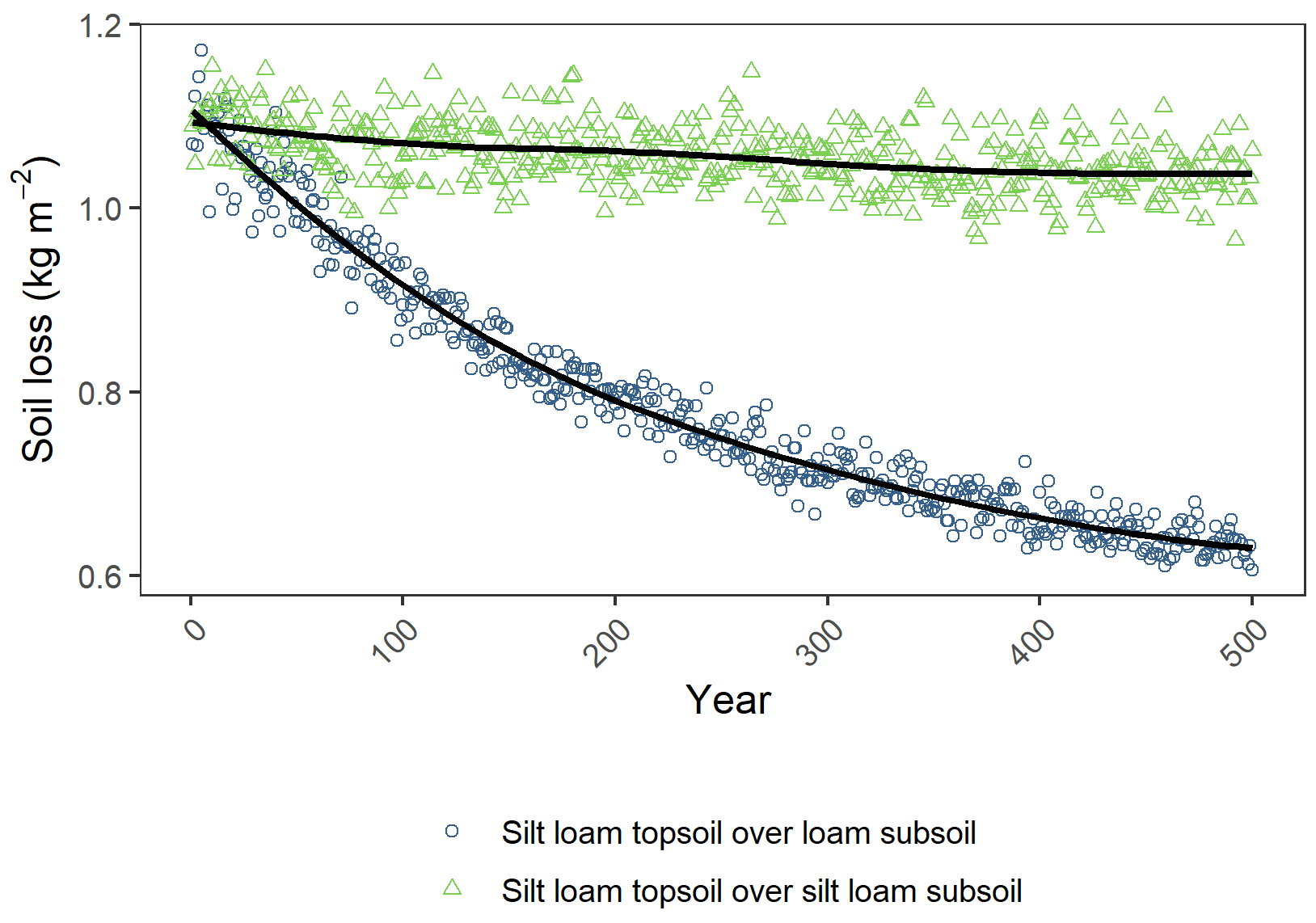
Figure 6 Soil erosion trends over 500 years of model simulations for two representative profiles from the UK SOILPITS dataset. Coloured symbols are the median of the simulations per year, and the solid lines are local regression functions adjusted from the data.

In order to understand the processes driving the soil erosion feedback system, we used a random forest analysis to rank the importance of model parameters for predicting the changes in soil erosion rates between the first and final time steps of the simulations. In this case, the differences between soil parameter values for the initial and final time steps were used as explanatory variables. All model simulations and statistical analyses were performed in R (R Core Team, 2022), and the model code is available as supplementary material (Batista et al., 2022).

Importantly, we did not consider all potential changes to the modelled systems. That is, we did not consider any feedbacks between soil thinning and crop development, nor the effects of climate change on rainfall, temperature, and farming practices. Although we are aware that such factors would likely have an impact on the model simulations, our aim here is to analyse the sensitivity of modelled soil losses to erosion-induced changes to soil properties. This involves making fixed assumptions about other system components. In addition, we would like to highlight that our model simulations should not be mistaken as projections of future erosion rates in Britain due to all the above-mentioned reasons.

3 Results

From the 265 soil profiles in the UK SOILPITS database, 262 (99 %) displayed a significant correlation (p<0.00001) between soil truncation and annual soil losses, of which 261 presented a decelerating feedback trend (Pearson's r<0). Considering the median of the simulations from all soil profiles, the temporal evolution of erosion rates was characterised by an exponential decay function (Fig. 5), which meant erosion rates initially decelerated at a higher pace until reaching a horizontal asymptote at approximately 250 years into the model runs. Based on the adjusted decay function, the initial soil loss rates (intercept = 0.81 kg m⁻² yr⁻¹) decrease in 6 % and 10 % over the first 50 and 100 years of the simulations, respectively; but there is only a decrease of 3 % in the last 100 years.

The changes in simulated soil losses between the initial and final model time steps per profile followed a normal distribution, which signified an average 20±8 % decrease in erosion rates. The steepest declines in soil losses (maximum 46 %) typically occurred in soil profiles with a negative gradient in silt contents in their subsoil horizons. Contrarily, the soil profiles with a stable erosion progression or with a gentler decay steepness were associated with the presence of silty substrata. Figure 6 illustrates the typical behaviour of these trends using data from two representative soil profiles with similar topsoil but with different subsoil properties at the beginning of the simulations.

It follows that simulated changes in erosion rates were largely explained by alterations in soil texture. This is demonstrated in Fig. 7, which displays a random forest importance ranking for predicting the differences in erosion rates between the initial and final time steps of the simulations, for each soil profile. The random forest analysis described how soil erosion responses were highly influenced by variations in silt content and stone cover. Changes in soil moisture at field capacity and bulk density had a lower impact on the modelled soil losses (Fig. 7).

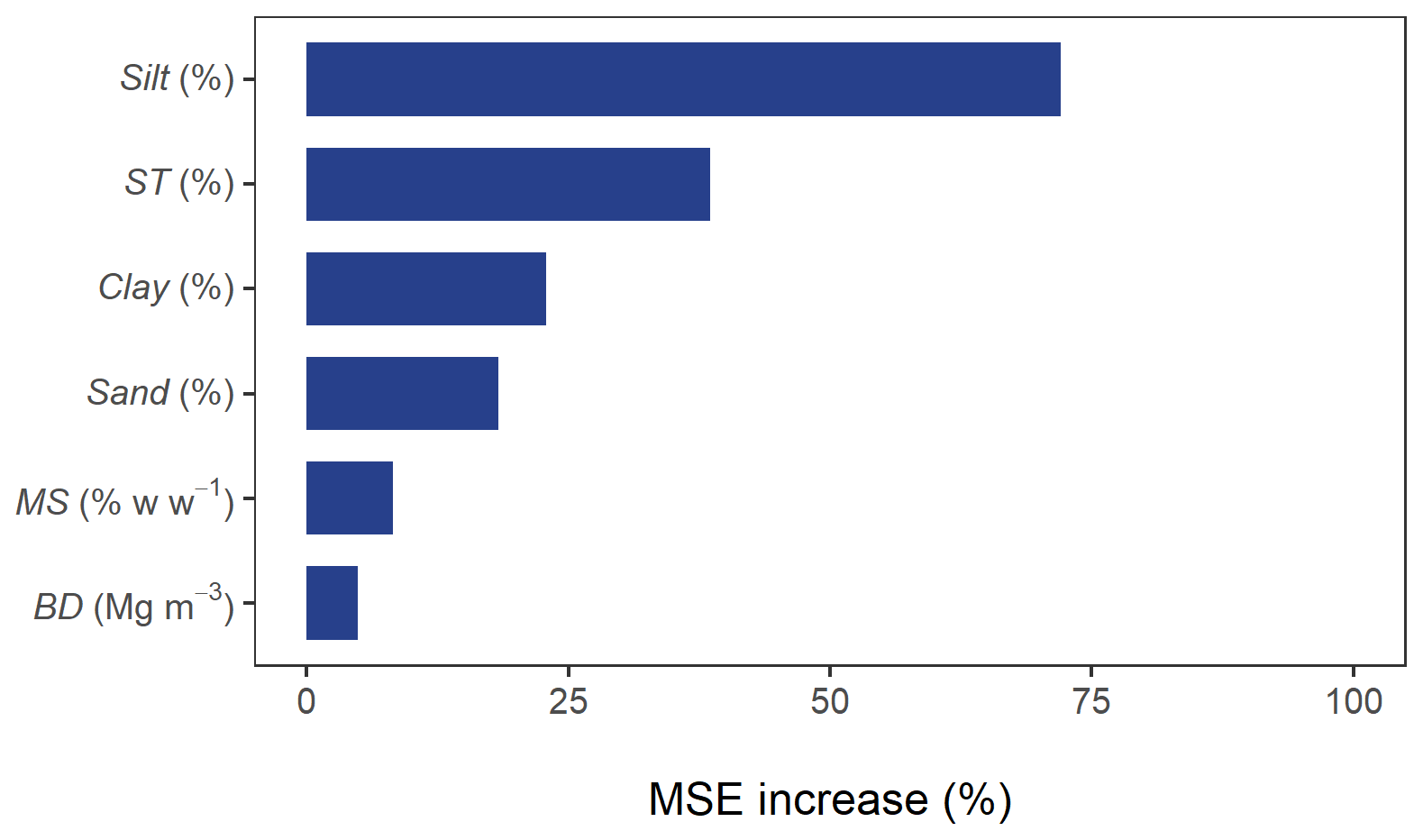
Figure 7 Random forest importance ranking for predicting the differences in erosion rates between the initial and final time steps of the simulations, for each soil profile. Feature importance is represented by the relative increase of the mean squared error (MSE) of the random forest (i.e. how much removing the feature increased the prediction error).

The sensitivity of the simulated changes in soil erosion rates to the erosion-induced changes to soil properties can be further visualised by comparing the difference in model parameter values with the variation in soil losses over 10-year rolling means (Fig. 8). Positive and negative changes in single parameter values did not yield consistent responses regarding the simulated soil losses (e.g. a 1 % decrease in sand content can lead to both accelerating and decelerating erosion rates over the rolling means). However, the direction of the changes in model parameters explains the general decelerating trend for the profiles (Fig. 8). For instance, the profile trajectories were characterised almost exclusively by decreasing contents of silt and increasing stone cover within the rolling means which led to net decreases in soil losses over the whole simulation period. Clay and sand contents mostly increased within the 10-year rolling means, although such a pattern was less pronounced compared to the silt and stone cover progressions. Less important parameters, such as bulk density and soil moisture at field capacity, displayed a more centred pattern along the y axis (Fig. 8).

Figure 8 Hexagonal heatmaps relating the changes in model parameters to soil loss responses over 10-year rolling means for the soil profiles. Colours represent the number (n) of cases in each hexagon.

The main processes driving the soil erosion feedback systems were particle detachment by raindrop impact and silt sediment supply (R²=0.85 and 0.66, respectively; Fig. 9), while changes in runoff amounts, detachment by runoff, and runoff transport capacity had a narrow effect on the simulated soil losses (Fig. 9). That is, only acute changes in discharge seem to have produced a sufficient response in detachment by runoff and in transport capacity to influence the net erosion rates (Fig. 9).

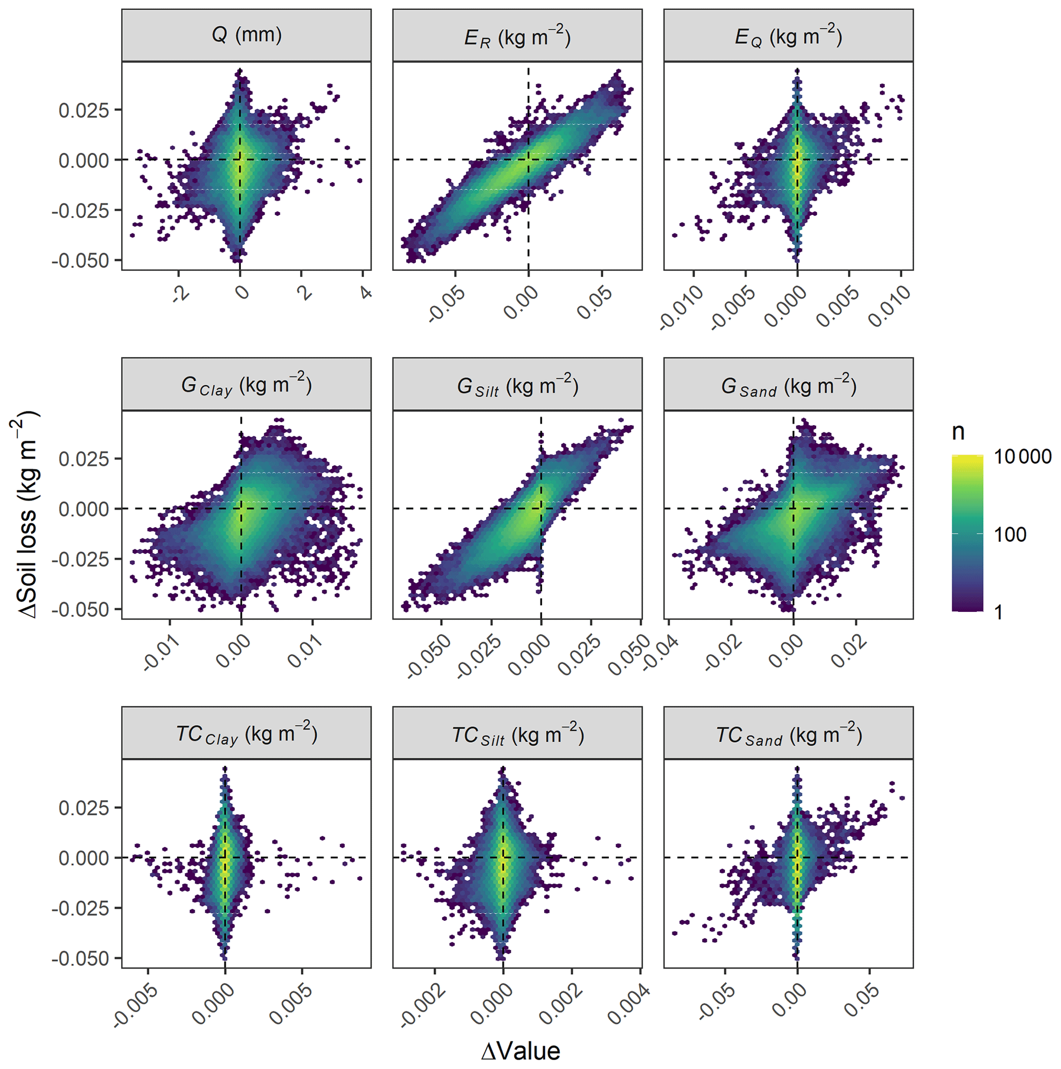
Figure 9 Hexagonal heatmaps and linear regression lines (p<0.00001) of the changes in soil loss over 10-year rolling means for the soil profiles. Colours represent the number (n) of cases in each hexagon.

Annual runoff depths and soil losses were correlated in 187 (71 %) of the 265 soil profiles (p<0.00001); however, these correlations did not amount to causation. The positive correlations (44 profiles; 17 %) occurred for instance when the uprise of clayey subsurface horizons led to a reduction in both runoff amounts (due to an increase in soil moisture storage capacity) and soil detachment. The negative correlations (143 profiles; 54 %) occurred due to selective erosion processes, soil organic carbon depletion, and the presence of sandy soil substrata. That is, as the silty material was removed, enriching the topsoil with sand and carbon-depleted subsoil, particle detachment by raindrop impact declined, whereas runoff amounts increased due to a reduction in soil moisture at field capacity. However, this increase in runoff was not sufficient to accelerate soil losses (Fig. 10).

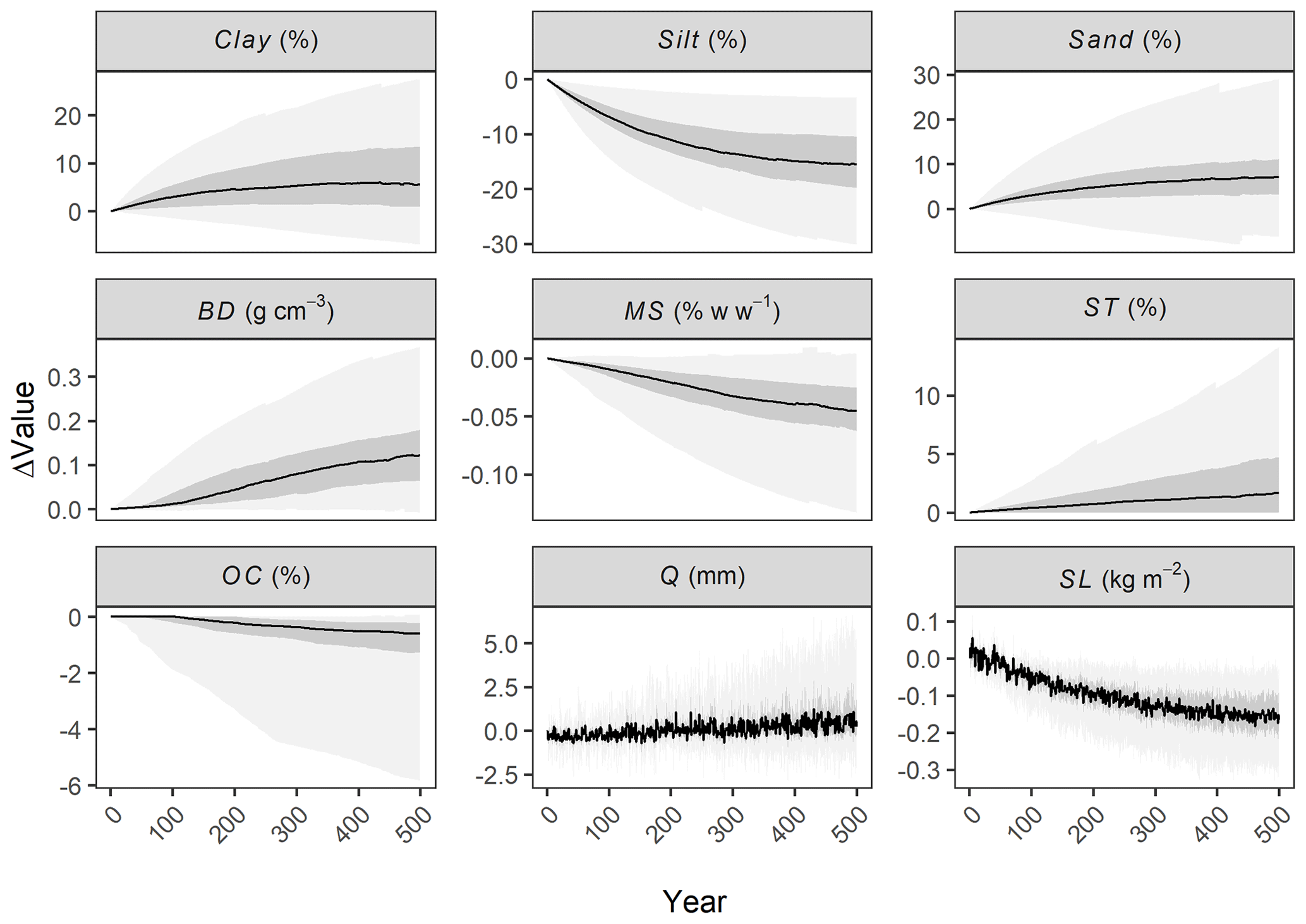
Figure 10 Annual changes in model parameter values and simulated runoff depths and soil losses over 500 years for the soil profiles from the UK SOILPITS database. The solid dark line represents the median of all profiles and simulations, whereas the shaded dark- and light-grey areas are 50 % and 95 % prediction intervals, respectively.

4 Discussion

Our model simulations underline the strong interaction between current soil erosion dynamics and the erosion history of soil profiles. In particular, the simulations demonstrate how different soils are likely to have contrasting responses to soil thinning, depending on the properties of the surface material, as well as those of the underlying soil horizons. In our database, most of the soil profiles presented a decelerating feedback trend, which reflects both the characteristics of these soils and, importantly, our basic modelling assumptions.

For instance, as silt detachability in the MMMF model is assumed to be much higher than for other particle size fractions, silt was preferentially removed from the soil matrix. In addition, as silt contents typically remain stable or decrease in the subsurface horizons of the soil profiles in our database (Fig. 2), silt was often not replenished by the underlying substrata being mixed into the plough layer. Such behaviour is overall consistent with empirical observations of selective particle size removal by interrill erosion processes (Koiter et al., 2017) and the progressive depletion of readily erodible material from eroding surface soils (Parsons et al., 1991). However, it is worth highlighting that the soil detachability values used in MMMF have a limited empirical basis (Quansah, 1982), and the erodibility of the clay particles might be poorly described due to the neglection of other variables, such as aggregate stability (Morgan and Duzant, 2008).

The residual accumulation of rock fragments further contributed to the reduction in erosion rates in the model simulations, as stone cover is assumed to armour the land surface and to reduce soil detachment. Specifically, even a small number of rock fragments in the soil matrix can disperse the overland flow and dissipate its energy, reducing rill incision and soil losses (Rieke-Zapp et al., 2007). Moreover, decreases in water erosion rates due to a residual increment of stone cover have previously been simulated by Govers et al. (2006), who warned, however, that the accumulation of rock fragments in arable soils depends on tillage practices. Notwithstanding, increases in rock fragment contents might also affect soil hydraulic conductivity and water holding capacity (Cousin et al., 2003), and therefore influence runoff formation. None of these potential interactions were represented in our model simulations, and might therefore warrant further scrutiny.

The few soil profiles displaying a stable or slightly accelerating erosion trend were characterised by the presence of sandy or loamy surface horizons over a siltier substratum, which successively supplied the plough layer with readily erodible material as the original topsoil was removed by erosion. Moreover, these profiles were defined by the absence of a surface stone cover and by subsoil horizons with very limited amounts of rock fragments. Although accelerating erosion trends were only simulated for one profile in our modelling experiment, such behaviour might be expected in soils with highly incrementing silt contents in their C horizons, which are common, for instance, where loess is the parent material (Finke, 2012; Świtoniak et al., 2016).

Moreover, potential accelerating erosion trends might have been under-detected by the model simulations, as we did not consider how truncation can decrease the soil moisture storage capacity due to a reduction in soil depth and how this might affect runoff generation (Dunne and Black, 1970; Morgan et al., 1984). That is, as soils become shallower, saturation-excess overland flow might increase, depending on the permeability of the bedrock or the presence of an impeding horizon (Beven, 2012; Moraes et al., 2010). We did not consider these processes in our simulation due to the absence of an explicit soil thickness parameter in the MMMF equations and the lack of data regarding the permeability of the soil profiles' parent materials. Although simulated increases in runoff formation were generally not sufficient to increase particle detachment by overland flow and soil losses in the model outputs (Figs. 9 and 10), different results would be conceivable at a landscape scale. For instance, if upslope run-on is considered, increases in overland flow due to soil truncation might lead to rill initiation in flow accumulation zones, which would largely increase the simulated erosion rates.

Furthermore, very different runoff responses to soil truncation can be expected in areas where infiltration excess is the dominant overland flow mechanism. While saturation excess is common under British edaphoclimatic conditions, most subhumid and semiarid zones are prone to the formation of infiltration-excess runoff, which is a process primarily controlled at the soil surface (Smith and Goodrich, 2005). Under such circumstances, erosion-induced changes to topsoil properties might have an even greater interaction with runoff generation. In particular, soil crusting slows down infiltrability and rapidly increases the overland flow, leading to greater soil losses (Le Bissonnais, 2016; Fiener et al., 2008; Veihe et al., 2001). As the development of soil crusts is influenced by soil texture and organic carbon content (Fiener et al., 2011), the truncation-induced changes we have simulated would likely alter the susceptibility of surface soils to crusting and, consequently, to the formation of infiltration-excess runoff. Another caveat in the model structure worth highlighting is that, different to model outputs, an uprise of subsurface clayey material might in fact increase infiltration-excess overland flow, due to the lower infiltrability and saturated hydraulic conductivity of heavy-textured soils (Hao et al., 2020), which are also more susceptible to compaction, depending on their mineralogy (Bonetti et al., 2017; Hamza and Anderson, 2005).

In addition, accelerating erosion responses to soil truncation might have been more frequent if we assumed an increase in topsoil erodibility due to the lower aggregate stability and looser structure of the carbon-depleted subsurface material being incorporated into the plough layer (Le Bissonnais, 2016; Doetterl et al., 2016; Tanner et al., 2018). That is, as the soil detachability coefficients from MMMF do not take soil organic carbon into account, the sensitivity of topsoil erodibility to soil truncation was likely downplayed. For instance, Radziuk and Switoniak (2021) used an equation from the Erosion Productivity Impact Calculator (EPIC) model to estimate the erodibility of Luvisols at different truncation stages in Poland. They found that more truncated soils had higher erodibility, due to decreases in soil organic carbon and sand content in the eroded Ap horizons.

Our model simulations may have particularly underestimated erosion responses to soil thinning for the profiles which displayed an accumulation of sand and a depletion in clay and silt contents. This progressive coarsening should lead to lower soil water availability, and therefore, lower soil cover, lower crop biomass production, and less organic carbon input from plants. As sandier soils already have less carbon stabilisation mechanisms (Doetterl et al., 2016), this would lead to even greater truncation-induced depletions in soil organic carbon and therefore increases in erodibility (Auerswald et al., 2014; Fernández and Vega, 2018). In general, as organic carbon was only an indirect model input via the PTFs for estimating bulk density and soil moisture at field capacity, the interplays between soil thinning, soil organic matter, and soil erodibility were likely underrepresented here.

Although not all the complex interactions between soil erosion and soil thinning could be described in our model, the simulated trajectories of erosion-induced changes to soil properties (Fig. 10) are consistent with field-observations. That is, measured data from eroded Ap horizons typically indicate (i) incrementing clay, sand, and rock fragment contents, (ii) increasing soil bulk density, (iii) depleting soil organic carbon contents, and (iv) decreasing soil water holding capacity with increasing erosion severity (Lowery et al., 1995; Rhoton and Tyler, 1990; Stone et al., 1985; Strauss and Klaghofer, 2001). Moreover, the decelerating erosion trend in our model outputs corroborate the results from Govers et al. (2006), who simulated an exponential decay in sediment production from arable hillslopes over a period of 50 years following land use intensification due to a rapid emergence of a soil with high stone cover. Importantly, the soil losses estimated from our model outputs (median =0.67 kg m⁻² yr⁻¹; interquartile range $=\mathrm{0.58}-\mathrm{0.80}$ kg m⁻² yr⁻¹) are encompassed by the median and the upper quartile of measured erosion rates from arable land at plot scale in the UK (∼0.1–1 kg m⁻² yr⁻¹) (see Benaud et al., 2020). We compare model outputs to plot-scale measurements due to their similarity with our modelling spatial unit (i.e. 10 m eroding hillslope segment with 6^∘ or 10.5 % slope gradient). It is worth highlighting that (i) the plot data described in Benaud et al. (2020) are mostly derived from slopes below 10 % and (ii) measured erosion rates at field or catchment scale in Britain are much lower than our model simulations.

Moreover, our model outputs further help to identify where more empirical evidence would help constraining modelling assumptions and improve process representation. For instance, investigating how truncation affects the aggregate stability of surface soils (due to changes in soil texture, mineralogy, and organic carbon dynamics) might be an important step in order to further understand the feedbacks between erosion and soil thinning. Interactions between soil truncation, water availability to plants, and crop growth – and how these could in turn reduce soil cover and organic carbon input – might also warrant further investigations. Similarly, exploring the responses of different runoff generation mechanisms to soil thinning and erosion-induced changes to soil properties should be beneficial to increase our understanding of the erosion feedback system. Modelling-wise, an important next step would be to adapt the framework described here into spatially distributed soil erosion models, in order to evaluate the effects of soil erosion feedback systems at landscape or watershed scale. This would allow for an unravelling of different feedback processes at different positions in the landscape, which might be affected by erosion-induced changes to soil properties in different ways.

Finally, although our model simulations indicate that soil thinning has a decelerating effect on soil loss rates for eroding hillslope segments in the UK, the results also demonstrate that some of these soils' physical properties might become restrictive for agriculture before the profiles are completely truncated. That is, some simulated erosion progressions create dense Ap horizons (max. bulk density of 1.78 M m⁻³) with excessive rock fragment contents (max. 36 %), very high clay (max. 89 %) or sand contents (max. 99 %), and low water holding capacity (min. soil moisture at field capacity of 0.14 % w w⁻¹). For such scenarios, rehabilitation techniques based on topsoil replacement might be necessary to sustain crop production (Schneider et al., 2021). These significant changes in soil properties, simulated in relatively short time periods (Fig. 10), further indicate how accelerated erosion in agricultural landscapes can potentially affect soil classification (Lewis and Witte, 1980; Olson and Nizeyimana, 1988; Świtoniak et al., 2016), which is important to consider when interpreting decades-old soil maps. Since soil erosion rates in Britain are much lower compared to other regions of the world (Benaud et al., 2020), our model simulations represent a somewhat conservative scenario of erosion feedback systems. Erosion-induced changes to soil properties, and their implications for modelling, should be particularly relevant in areas under severe erosion rates.

5 Conclusions

Here, we explored the soil erosion feedback system in 265 agricultural soil profiles in the UK. In particular, we simulated how selective erosion processes and the incorporation of different subsoil horizons into the plough layer affected the erodibility of surface soils. We further analysed how these processes could change erosion rates during a period of 500 years. We found that (i) soil erosion rates in 99 % of the soil profiles were sensitive to soil truncation, (ii) the truncation-sensitive profiles essentially displayed a decelerating trend, and (iii) changes in soil texture and stone cover were the main drivers of the modelled soil erosion feedbacks loops. Importantly, we found that different soils had different simulated responses to soil truncation, depending on the properties of the surface material as well as those of the underlying soil horizons.

Ultimately, our findings highlight the dynamic nature of the soil as a three-dimensional body. That is, even the so-called intrinsic properties of surface soils might change in a matter of decades in areas under accelerated erosion rates. Moreover, erosion-induced changes to soil properties can have a significant impact on the rates with which soils are eroded, which in turn affects the calculation of soil lifespans and model-based erosion projections. Therefore, understanding how erosion-induced changes to soil properties reverberate with erosion itself will be crucial for improving long-term model predictions, investigating the resilience of different soils to erosion disturbances, and for developing appropriate soil conservation strategies for a changing world.

Appendix A

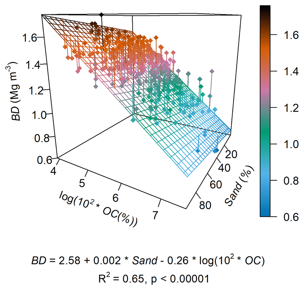
Figure A1 Pedotransfer function for estimating bulk density (BD) as a function of sand and organic carbon (OC) content. The regression was fit using only the data for the A horizons in the 265 agricultural soil profiles from the UK SOILPITS dataset used in this study

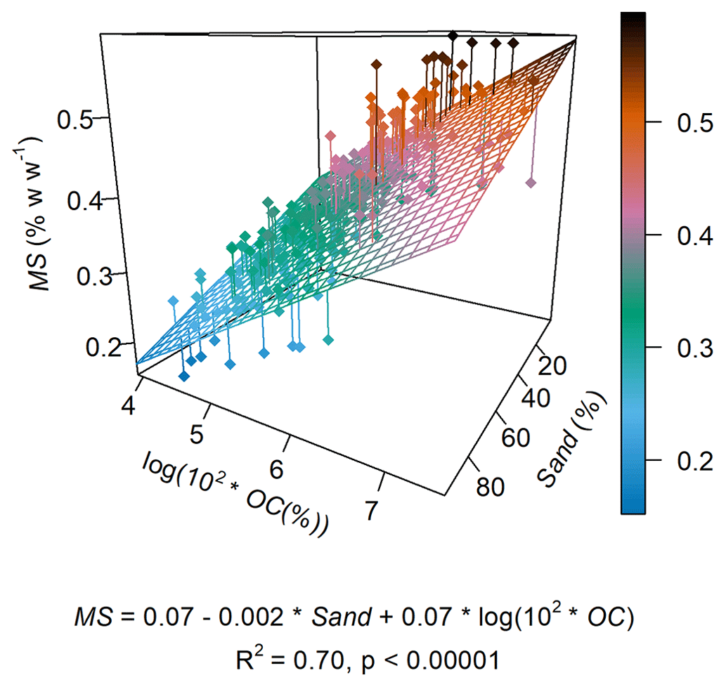
Figure A2 Pedotransfer function for estimating soil moisture at field capacity (MS) as a function of sand and organic carbon (OC) content. The regression was fit using only the data for the A horizons in the 265 agricultural soil profiles from the UK SOILPITS dataset used in this study.