the Creative Commons Attribution 4.0 License.
the Creative Commons Attribution 4.0 License.
 | 17 Nov 2022
Improving models to predict holocellulose and Klason lignin contents for peat soil organic matter with mid-infrared spectra
Henning Teickner
Klaus-Holger Knorr
To understand global soil organic matter (SOM) chemistry and its dynamics, we need tools to efficiently quantify SOM properties, for example, prediction models using mid-infrared spectra. However, the advantages of such models rely on their validity and accuracy. Recently, Hodgkins et al. (2018) developed models to quantitatively predict peat holocellulose and Klason lignin contents, two indicators of SOM stability and major fractions of organic matter. The models may help to understand large-scale SOM gradients and have been used in various studies.
A research gap to fill is that these models have not been validated in detail yet. What are their limitations and how can we improve them? This study provides a validation with the aim to identify concrete steps to improve these models. As a first step, we provide several improvements using the original training data.
The major limitation we identified is that the original training data are not representative for a range of diverse peat samples. This causes both biased estimates and extrapolation uncertainty under the original models. In addition, the original models can in practice produce unrealistic predictions (negative values or values >100 mass-%). Our improved models partly reduce the observed bias, have a better predictive performance for the training data, and avoid such unrealistic predictions. Finally, we provide a proof of concept that holocellulose contents can also be predicted for mineral-rich samples (e.g., peat with mineral admixtures or potentially mineral soils).
A key step to improve the models will be to collect training data that are representative for SOM formed under various conditions. This study opens directions to develop operational models to predict SOM holocellulose and Klason lignin contents from mid-infrared spectra.
- Article
(2141 KB) - Full-text XML
-
Supplement
(19020 KB) - BibTeX
- EndNote


Understanding soil organic matter chemistry and how it changes is important to understand future global carbon dynamics. The chemistry of soil organic matter (SOM) controls how fast it can be decomposed (Bengtsson et al., 2018; Shipley and Tardif, 2021). To understand and predict these processes, we therefore need to measure SOM chemistry on a global scale. A challenge is that soils develop under diverse and changing environmental conditions which also affect SOM quality (Scharlemann et al., 2014; Lehmann and Kleber, 2015). As a consequence, spatially and temporally resolved measurements on a global scale are needed. For this, we need methods to measure SOM chemistry efficiently.
Mid-infrared spectra (MIRS)-based models to predict SOM properties are a promising high-throughput approach which can replace more labor intensive or costly measurements (Viscarra Rossel et al., 2006). For example, MIRS have been used to predict elemental contents which otherwise are measured using e.g., combustion and gas chromatographic analysis of resulting gases. However, all the advantages of MIRS-based models rely on the accuracy of the computed models. This makes model validation a crucial step during model development.
Soil and plant OM is often characterized by step-wise chemical fractionation into holocellulose (acid soluble) – a proxy for polysaccharides – and lignin (acid insoluble) – a proxy for aromatics – (De la Cruz et al., 2016; Elle et al., 2019), and these variables are often important indicators for the chemical quality of OM in studies and models analyzing decomposition of SOM (Leifeld et al., 2012; Biester et al., 2014; Worrall et al., 2017; Hodgkins et al., 2018; Bengtsson et al., 2018; Ågren et al., 1996; Bauer, 2004; Shipley and Tardif, 2021). If these fractions can be predicted from MIRS, it may be possible to understand decomposition across larger scales and at higher spatial resolution.
Several models to predict holocellulose and lignin contents in different OM types have been developed (some based on near infrared spectra) (summarized for lignin by Elle et al., 2019; for holocellulose see e.g., Peltre et al., 2011; Sun et al., 2011). Most of these models consider only wood, material from few woody and non-woody species, or only specific vegetation organs (Elle et al., 2019). Another problem is that most of these models cannot be easily reproduced and used since the raw data and code have not been published.
Recently, Hodgkins et al. (2018) developed models to predict Klason lignin and holocellulose contents from attenuated total reflectance MIRS. The models have several advantages over existing approaches. The training data comprise several different OM types, such as paper products (cardboard, office paper, magazines, newspaper), leaves from diverse species (trees and graminoids), and wood samples (De la Cruz et al., 2016; Hodgkins et al., 2018). Moreover, both raw data and model code are publicly available (Hodgkins et al., 2018; Teickner and Hodgkins, 2020). For this reason, the models are particularly suitable for application in other studies (Teickner et al., 2019; Moore et al., 2019; Harris et al., 2020; Cong et al., 2020, 2022), most recently in Verbeke et al. (2022) and Baysinger et al. (2022), and for future developments, e.g., by including additional data.
A major problem is that neither Hodgkins et al. (2018), nor any later study which was cited above and which used the models, provided a thorough validation of the models. To compute the models, Hodgkins et al. (2018) developed a procedure to extract peaks which are indicative for specific OM fractions, such as holocellulose and Klason lignin (Fig. 1), from the MIRS. In the procedure, the peaks are baseline corrected, their maximum height computed, and normalized – divided by the sum of absorbance values in the spectra. In Hodgkins et al. (2018), these values were used to calibrate the prediction models. As model validation, only the linearity between the target variables and predictors was assessed (Supplement to Hodgkins et al., 2018), but not, for example, how predicted values match measured values. Moreover, no information has been provided whether the training data are representative for SOM, particularly the peat samples analyzed in the study. Furthermore, it is unclear if pre-selecting peaks may reduce the predictive accuracy of the models. Many of these concerns have also been raised by an anonymous reviewer of the paper (Supplement to Hodgkins et al., 2018). Thus, an important research gap to fill is to validate the models and to provide concrete strategies for further improvements.

Figure 1Sample spectrum with the peaks and troughs, their heights, and their baselines (green) as detected by the script developed by Hodgkins et al. (2018). The plot was created with the data and code from Hodgkins et al. (2018) as implemented in ir and irpeat, respectively.
Our goals are to identify limitations in the original models and to give concrete recommendations for improvements. Moreover, we use the original data from Hodgkins et al. (2018) to provide improvements on the original models where possible. To this end, we conducted an exploratory analysis using the peat and peat-forming vegetation data provided by Hodgkins et al. (2018). Our exploratory analysis was guided by the following research questions.
-
Is the normal distribution reasonable to predict holocellulose and Klason lignin contents for peat samples? Klason lignin and holocellulose contents as actually measured for the training data set in Hodgkins et al. (2018) cannot be negative or larger than 100 mass-%. For this reason, predictions and prediction uncertainties of the models should be in the interval [0, 100] mass-%. Yet, the original models assume a normal distribution which does not entail any lower or upper bound for predicted values. This can potentially result in unrealistic predictions. However, if no unrealistic predictions occur for “representative” peat samples, using a model with normal distribution can be justifiable in practice. In contrast, if unrealistic predictions occur, it is more reasonable to use a distribution for which assumptions are consistent with knowledge on the data-generating process. For example, the beta distribution assumes a lower and upper bound which can be mapped to the interval (0, 100) mass-%. It can be used as replacement for the normal sampling distribution used in ordinary linear regression models, such as the original models. For this reason, we were interested if and under which conditions the original models may produce unrealistic predictions for the peat and vegetation samples.
-
Can the predictive accuracy of the models be improved? The original models were parameterized with manually selected variables (normalized peak heights from the extraction procedure) (Hodgkins et al., 2018): the peak
carb(∼ 1090 cm−1) for holocellulose and the sum of the peaksarom15(∼ 1515 cm−1) andarom16(∼ 1650 cm−1) (arom15arom16) for Klason lignin. Whilst there is both a strong causal rationale behind this decision and it may support the robustness of the models (Hodgkins et al., 2018), it is also under risk of underfitting – excluding informative variables and thus missing an opportunity to improve predictive accuracy. For this reason, we were interested if including more variables extracted from the MIRS results in models with a better predictive accuracy. -
Is the prediction domain of the training data representative for peat samples? If a model extrapolates outside the prediction domain – the range of predictor variable values in the training data set (Wadoux et al., 2021) – it is unclear if the predictions are valid. An advantage of the independent reference sample set used by Hodgkins et al. (2018) is that the model is applicable to various OM types and, for example, does not depend on obviously material-specific spectral characteristics (Hodgkins et al., 2018). For example, in peat, holocellulose content is controlled by decomposition, and other structures also controlled by decomposition might therefore provide information on holocellulose contents (Leifeld et al., 2012; Biester et al., 2014). However, this does not have to be the case for other samples, e.g., peat-forming vegetation. A potential advantage is therefore the potential generality of the training data set Hodgkins et al. (2018) used. However, since it does not include peat samples, it is questionable if the prediction domain formed by the training samples covers peat samples and peat-forming vegetation in general, and this can result in overlooking prediction failures due to extrapolation. For this reason, we were interested if the training data (its prediction domain, Wadoux et al., 2021) is representative for peat and peat-forming vegetation.
-
Do predictions of the improved models differ and, if so, why? Computing modified models enables us to compare their predictions to those of the original models using the same training data and to the actually measured contents. Model comparison often reveals detailed insights into the mechanics of a model and may provide hints to which model makes more correct predictions. We therefore were interested in analyzing differences between the computed models, what factors may cause differences in predictions, and if there are indications of which models make more correct predictions.
-
Can holocellulose contents also be predicted for samples with mineral interferences? During model calibration, Hodgkins et al. (2018) omitted some samples. For prediction of holocellulose, old magazine samples were omitted because the
carbpeak suffered from mineral interference from the samples' clay coatings (Hodgkins et al., 2018). This decision is sensible, but since there are many organic soils with mineral admixtures – for example, due to volcanic ash, in base layers, or due to cryoturbation) (e.g., Broder et al., 2012; Bockheim, 2007; Koven et al., 2009; Loisel et al., 2014) – we think that it is useful to have a model to predict holocellulose contents that includes mineral-rich samples. We therefore wanted to investigate if a suitable model can be computed by including the previously omitted old magazine samples during calibration. This is no replacement for a model using more training data, but it is a test whether it is at least in principle possible for MIRS to contain sufficient information to predict holocellulose contents of relatively diverse samples.
In investigating these issues, our main goals are to provide a concrete plan for how to improve the original models. Moreover, we want to analyze under which conditions it may not be appropriate to use the original or modified models. Where possible, using the original data, we want to provide improved models which we hope can be further improved in the future. In addition, this study provides general guidance for pitfalls during validation of spectral prediction models. With this, we want to contribute to the development of models to predict SOM holocellulose and Klason lignin contents which are important to provide diverse data to fit SOM decomposition models and to understand how environmental change affects global soil carbon dynamics.
We conducted a series of statistical analyzes to query each of our research questions listed in the introduction. During this, we also computed improved models using the same training data that were used to compute the original models. Since we used these improved models to uncover and analyze the limitations in the original models, we first describe the steps of how we improved the original models and then how we analyzed the limitations.
We use the data and models collected and developed by Hodgkins et al. (2018). The training data used to calibrate the original models consist of various organic materials and comprise measured values for holocellulose and Klason lignin (De la Cruz et al., 2016). The data are accessible from the Supplement of Hodgkins et al. (2018). In addition, we used a data set consisting of MIRS for 14 peat cores (300 samples in total) and 39 vegetation samples collected at the same sites which are also provided by Hodgkins et al. (2018). We used these peat and vegetation data to evaluate the performance of the original and improved models for peat and peat-forming vegetation in general. We assume that the peat samples are representative for a wide range of peat OM because they cover a large latitudinal range and a wide range of degrees of decomposition, and were formed by different vegetation (Hodgkins et al., 2018).
We computed all models as Bayesian models. This allowed us to consider parameter uncertainty in predictions and to compute models with good predictive performance (Raftery and Zheng, 2003; Piironen and Vehtari, 2017a). For this reason, to facilitate model comparison, we also recomputed the original models as Bayesian models with weakly informative priors. With weakly informative priors, we mean here priors which result in approximately the same prediction intervals as the original frequentist models (Supplement Fig. S1). Whenever we refer to “original model”, we mean these Bayesian translations, and otherwise refer to “original non-Bayesian models”. To check that we did not introduce any of the identified weaknesses using the Bayesian approach, we compared the predictions of the Bayesian models to the original non-Bayesian models (Supplement Fig. S1).
All analyzes were performed in R (version 4.0.1, 6 June 2020) (R Core Team, 2020). Spectra were preprocessed using ir (0.0.0.9000) (Teickner, 2020). The original script used by Hodgkins et al. (2018) to extract peaks (https://github.com/shodgkins/FTIRbaselines, last access: 11 November 2022) as implemented in irpeat (0.0.0.9000) (Teickner and Hodgkins, 2020) was used to recompute the original models and extract peaks from MIRS. Bayesian models were computed using rstanarm (2.19.3) (Goodrich et al., 2020) and brms (2.13.0) (Bürkner, 2017, 2018) which are interfaces to Stan (2.21.0) (Stan Development Team, 2020, 2021). All predictor variables were z-transformed. Markov chain Monte Carlo (MCMC) sampling was validated in addition using bayesplot (1.7.2) (Gabry and Mahr, 2020). The out-of-sample predictive performance of the models was estimated using the expected log predictive density (ELPD) estimated using Pareto smoothed importance sampling leave-one-out cross-validation (PSIS-LOO) (Vehtari et al., 2017) using the loo package (2.2.0) (Vehtari et al., 2019). PSIS-LOO ELPD is an universal measure to compare the predictive performance of models and is the deviance (Vehtari et al., 2017).
2.1 Normal versus beta regression models
Above, we mentioned that assuming a model with normal distribution can result in unrealistic predictions outside the interval [0, 100] mass-%. We were interested if and under which conditions unrealistic predictions can occur. Here, we differentiate two ways in which a prediction can be unrealistic: it can be either an unrealistic point estimate (median predictions), or the prediction interval can cover values outside [0, 100] mass-%, even though the median prediction can be within [0, 100] mass-%.
For our analysis, we first computed a sequence of normalized carb and arom15arom16 peak heights such that the original model predicts values which completely covered the interval [0, 100] mass-% for holocellulose and Klason lignin, respectively. For these simulated peak heights, we computed median model predictions and 90 % prediction intervals using the original models (“original Gaussian models”). Finally, we identified unrealistic predictions in terms of the point estimates and 90 % prediction intervals and the carb and arom15arom16 peak heights under which these occur. We used these values as thresholds to decide if the models make unrealistic predictions in practice. To relate these values to real data, we computed median predictions and 90 % prediction intervals also for the peat and vegetation samples and identified unrealistic predictions as for the simulation analysis.
After identifying conditions under which unrealistic predictions occur, we compared this to the behavior of a model with assumptions in line with the data generating process. Beta regression models assume all values of the dependent variable to be in (0, 100) mass-% which is a reasonable assumption given how the actual data are generated. Therefore, we repeated the previous analyses, but now using beta regression models. We used the same model structure and priors for intercept and slopes as the original models (“original beta models”).
To facilitate practical comparison between the modeling approaches, we compared the predictions of all models for the peat samples by plotting predicted values versus depths of the peat samples. Altogether, this allowed us to identify unrealistic predictions of the original models and to analyze how the improved models (beta regression models) perform in comparison.
2.2 Reducing underfitting with more variables
The original approach of Hodgkins et al. (2018) was to include only manually selected variables which may result in underfitting and consequently relatively low predictive accuracy. We wanted to investigate if the predictive accuracy can be improved by including more variables in the models. Two approaches with complementary advantages and disadvantages were tested:
-
We used all peak heights and trough heights returned by the peak identification algorithm of Hodgkins et al. (2018) (Fig. 1). The advantage is that this makes the prediction model probably more robust against calibration transfer issues in comparison to the second approach (a hypothesis that remains to be tested). The disadvantage is that additional information contained within the spectra cannot be fully exploited if these are not contained within the extracted peak heights. To avoid overfitting, we computed models using priors implying different amounts of regularization – shrinking coefficients to 0 with the aim to avoid overfitting – of model coefficients (standard deviation of 1 and 0.5, respectively) in addition to the default weakly informative prior which we derived from rstanarm (2.19.3) (standard deviation of 2.5) (Goodrich et al., 2020).
-
We used all variables in the spectra and Bayesian regularization (Piironen et al., 2020), similar to Teickner et al. (2022). The advantage is that this approach can more fully exploit the information contained within the spectra because it is not restricted to specific peaks, resulting potentially in a better predictive performance. The disadvantage is that this approach may be more prone to calibration transfer issues. To reduce redundancy in the variables and impact of noise, we binned the spectra, testing bin widths of 10, 20, 30, 50, and 100 cm−1. As regularizing priors, we used the regularized horseshoe prior with a parameterization as described in Piironen and Vehtari (2017b), assuming a number of relevant variables of eight.
An alternative popular approach to approach 2 would be dimension reduction, for example, via partial least squares regression, principal component regression, or variants of these (Xiaobo et al., 2010). In general, there are many alternative approaches which could be tested to use more information contained within the spectra than the original models, and many of these probably would result in similar predictive performances as approach 2 (regularization), especially when sample sizes are small (Xiaobo et al., 2010; Teickner et al., 2022). An advantage of regularization is that model coefficients are estimated more independently than in dimension reduction approaches, which makes it more straightforward to interpret model coefficients. The key is that the approaches we chose are suitable to analyze our research questions.
Out-of-sample model performance was estimated with PSIS-LOO ELPD as described above (Vehtari et al., 2017, 2019). If a model has a larger PSIS-LOO ELPD than another model fitted on the same data, it has a larger (leave-one-out cross-validation) predictive accuracy, so models with larger PSIS-LOO ELPD are preferred (Vehtari et al., 2017). To compare models, one typically computes the posterior distribution of the difference in PSIS-LOO ELPD between the model with the largest PSIS-LOO ELPD and the other models, such that one can evaluate the probability of a certain predictive advantage of the best model in comparison to the other models (Vehtari et al., 2017, 2019).
To further validate and interpret the models using binned spectra, we visually identified the most important bins in the models (largest absolute median coefficients ≥0.2) with a bin width of 20 cm−1 (which are among the models with the best predictive accuracy; see below) and linked these to molecular structures and causal relations that most probably result in the correlation with holocellulose and Klason lignin, respectively.
Based on the model validation, we defined the following set of models used in the subsequent analyses: “best all peaks” denotes the models for holocellulose and Klason lignin with best average predictive accuracy of approach 1 described above. “Best binned spectra” denotes the models for holocellulose and Klason lignin with nearly the best average predictive accuracy of approach 2 described above. With “nearly the best predictive accuracy” we mean here that we used the models using binned spectra with a bin width of 20 cm−1. This was the model with best average predictive accuracy for Klason lignin, but not holocellulose (Sect. 3.2). However, the model for holocellulose had a predictive performance very similar to the on average better model using a bin width of 10 cm−1 (Sect. 3.2), and to keep the following analyses compact and easier to follow, we decided to use a bin width of 20 cm−1 in all cases. These models are the models used during the subsequent analyses.
2.3 Assessing the prediction domain of the training data
Are the training data used to compute the models representative for the spectral properties of peat and peat-forming vegetation? To answer this question, we needed to compare the spectral properties of the training samples to those of the peat and vegetation samples (Wadoux et al., 2021): if for a sample the value of a spectral variable included in a model exceeds the range of values for the same variable in the training data, the model extrapolates if applied to the sample (Wadoux et al., 2021). If extrapolation occurs, it is unclear if the predictions are valid estimates for holocellulose and Klason lignin contents.
For the original models, the prediction domain is simply the range of area normalized heights of the carb and arom15arom16 peak, respectively (Hodgkins et al., 2018). Therefore, we could directly compare the area normalized heights of the carb and arom15arom16 peak of the peat and vegetation samples to the range of area normalized heights of the same peaks for the training data.
For the improved models using binned spectra, the predictor variables form a multivariate prediction domain. We therefore created plots with which we could compare the value ranges for each bin for the training data with the respective values in the peat and vegetation spectra. This allowed us to identify for which spectral variables extrapolation is an issue. Finally, by identifying the most important variables in the improved models, we could qualitatively summarize how large the risk of this extrapolation is.
Since models with a bin width of 20 cm−1 were among the best models, we performed this analysis only for these models (“best binned spectra”). We did not additionally investigate the prediction domain for the models using all extracted peaks and troughs (“best all peaks”) since these models had no predictive advantage in comparison to the models using binned spectra (Sect. 3.2).
2.4 Analyzing differences in predictions between the original models and the improved models
We analyzed how predictions of the improved models (“best all peaks” and “best binned spectra” defined in Sect. 2.2) differ from the original models. We found considerable differences, even within the spectral range of the training data, and therefore analyzed what factors probably cause these differences.
In a first step, we were interested if the original or improved models are biased. Hodgkins et al. (2018) provide no plot of residuals against predicted values or measured values against predicted values. Both plots are commonly used to detect any biases in a model fit (e.g., Piñeiro et al., 2008). We therefore plotted measured values against predicted values for the original model and the improved model and compared indication of bias between both.
In a second step, we compared how predictions of the improved models differ in practice from the original models. To this end, we compared the models' predictions for the peat and vegetation data from Hodgkins et al. (2018), similarly to how we compared the Gaussian and beta regression models. Since we found considerable differences, we conducted a more targeted exploratory analysis to identify factors probably causing these differences.
2.5 Predicting holocellulose contents in samples with mineral admixtures
In the introduction we mentioned that the original Hodgkins et al. (2018) model for holocellulose excluded training samples with admixtures of clay minerals (old magazine samples) since these interfere with the carb peak. By including more variables into the model than the carb peak (as described in the previous section), we tried to compute models that can also describe the holocellulose content in the training data samples with high clay content. For this, we fitted the best models for holocellulose (the models in “best all peaks” and “best binned spectra” defined in Sect. 2.2) from each of the two approaches described in the previous section again, but this time including the four old magazine samples previously left out. We interpreted the coefficients of these binned models similarly to the versions not fitted with mineral-rich samples (see Sect. 2.2).
3.1 Is the normal distribution reasonable to predict holocellulose and Klason lignin contents for peat samples?
The original model for holocellulose indeed produced unrealistic predictions: it had a negative point prediction for one strongly decomposed sample from a tropical peat core. Moreover, for 22 % of the peat samples in the data from Hodgkins et al. (2018), the lower 90 % prediction interval covered negative values (Supplement Fig. S3). No point prediction or 90 % prediction interval was >100 mass-%. The original model for Klason lignin did not produce unrealistic predictions for the peat samples (Supplement Fig. S3). Both models did not produce unrealistic predictions for the vegetation samples.
Figure 2 shows predicted medians and prediction intervals for both models across a potential range of the spectral predictor variables alongside the range covered by the peat and vegetation samples. The model with normal distribution produces negative lower prediction interval limits whenever the predicted median is lower than around 17 mass-% and upper prediction interval limits >100 mass-% whenever the predicted median is larger than around 86 mass-%. For Klason lignin these values are around 9 mass-% and 87 mass-%, respectively.
The beta regression models produce realistic predictions across the complete range of the spectral predictor variables. In addition, the beta regression model has smaller prediction uncertainties for extreme values (Fig. 2). A consequence of this is larger predicted holocellulose contents with narrower prediction intervals for several (decomposed) peat samples under the beta regression model in comparison to the original normal model (Figs. 2 and S3).
Thus, whereas our results indicate little differences in choosing a model distribution for Klason lignin, for holocellulose contents of peat samples it is crucial to use a beta regression model to avoid unrealistic predictions. Nevertheless, it is generally advisable to use a beta regression model for mass contents. It may not be known in advance how large holocellulose or Klason lignin contents are for a given sample, and even for Klason lignin, contents may be low, e.g., due to high contents of minerals.
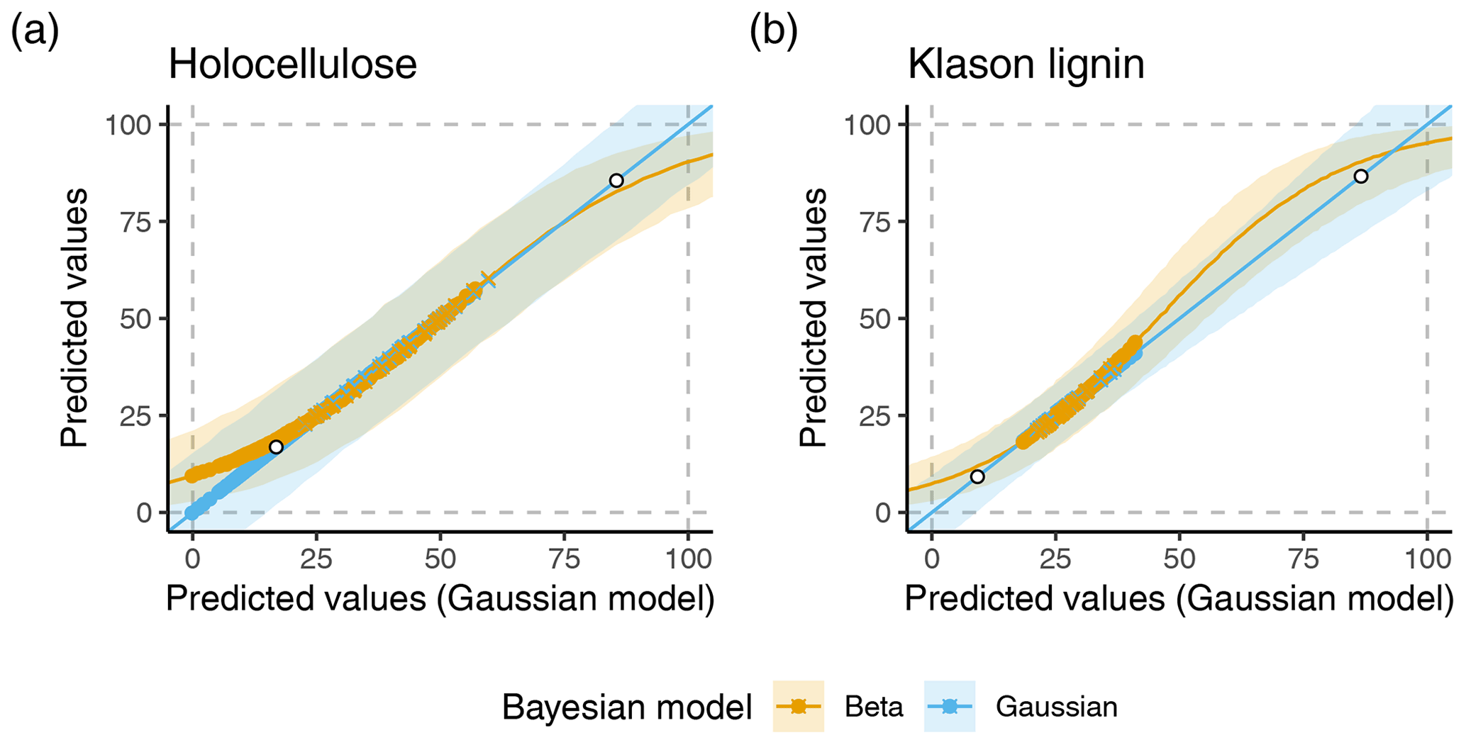
Figure 2Predicted holocellulose (a) and Klason lignin (b) contents using either the original Gaussian models or a beta regression model, versus predictions of the original Gaussian model covering the entire interval [0, 100] mass-%. Colored lines within shaded regions are median predictions. Shaded areas and boundaries are 90 % prediction intervals. Colored points are median point predictions for the peat (round points) and vegetation (crosses) samples from Hodgkins et al. (2018). Colors differentiate predictions of the original Gaussian model (blue) and the model with beta distribution (yellow). White filled points indicate the fitted values for which the 90 % prediction interval of the Gaussian model contains unrealistic values.
3.2 Can the predictive accuracy of the models be improved?
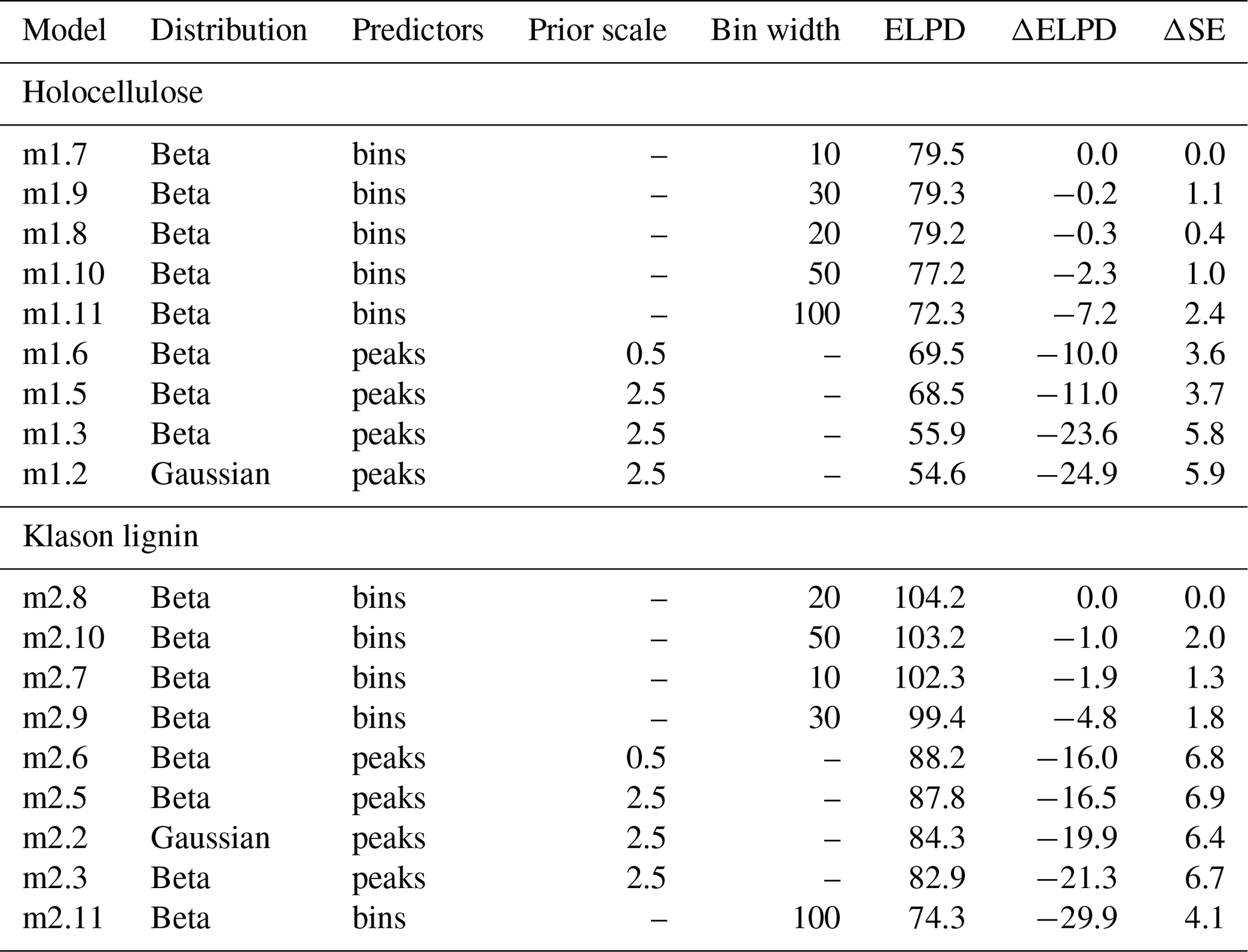
Our analysis shows that both strategies to include more variables result in on average more accurate predictions (Table 1). This can be concluded based on the average estimated ELPD values (larger values indicate a better estimated predictive accuracy). Consequently, using the data available, we could improve both the model for holocellulose and the model for Klason lignin.
Is one of the strategies to include more variables advantageous? The models with the largest predictive accuracy are models with small to moderate bin width (Table 1). These are better than the respective models using all extracted peaks: in addition to the ELPD, this can be derived from the standard errors of the ELPD differences relative to the best models (2⋅ΔSE is approximately the 95 % confidence interval). In addition, the remaining binned models generally have a better average predictive accuracy than the models using all extracted peaks, except for the model with bin width = 100 cm−1 for holocellulose. Summarized, this indicates that – if a sufficiently high bin resolution (sufficiently small bin width) is chosen – using binned spectra results in an improved predictive accuracy over approach 1 to use all extracted peaks for both holocellulose and Klason lignin.
To interpret the improved models using binned spectra, we plotted the median coefficients for the best models using binned spectra (Fig. 3). From this plot, we identified the bins with the largest absolute median coefficients (≥0.2, marked with points and labeled). The reason for the (on average) improved performance is that the improved models can use information contained in the complete spectra which is not contained in the manually selected peaks for the original models.
Similarly to the original model, a variable near the carb peak is important to predict the holocellulose content (bin at ∼ 970 cm−1) since it is related to cellulose (Cocozza et al., 2003; Stuart, 2004; Artz et al., 2008), but one peak related to aromatic structures which is not extracted with the approach from Hodgkins et al. (2018) is also important (∼ 1250 cm−1: aromatic in plane C–H bending) (Stuart, 2004) (Fig. 3a). This indicates that aromatics provide information on the holocellulose content in the training samples and that extracting only selected peaks may omit useful information. A plausible explanation for the importance of this variable is that holocellulose and Klason lignin together are the major mass fractions in many OM types and both are controlled by the same processes, but often in different directions (decomposition, resource allocation trade-off during plant growth, selective removal during processing) (Biester et al., 2014; Chen et al., 2016) (supporting Fig. 4).
For Klason lignin, the improved model does not use bins near to the arom15 and arom16 peaks, in contrast to the original model. Instead, bins with large absolute coefficients are located in the fingerprint region (600 to 1500 cm−1) and probably related to aromatic in plane C–H bending (∼ 1150 and ∼ 1270 cm−1) (Stuart, 2004) (Fig. 3c). A plausible explanation for the negative sign of the coefficient for the 1150 cm−1 bin is that absorbance in this range is partly caused by syringyl units (S) (Kubo and Kadla, 2005) and that training samples with higher S content have smaller Klason lignin contents (Supplement Fig. S4, De la Cruz et al., 2016), making this bin indicative of smaller Klason lignin contents. Likewise, a plausible explanation for the positive sign of the coefficient for the 1270 cm−1 bin is that absorbance in this range is caused predominantly by guaiacyl units (G) (Kubo and Kadla, 2005) and that training samples with higher G content have smaller Klason lignin contents (Supplement Fig. S4, De la Cruz et al., 2016), making this bin indicative of larger Klason lignin contents. In Sect. 3.5, we provide a mechanistic interpretation for why the selected variables are important.
The bins with especially large absolute coefficients in the models using binned spectra are not represented in the extracted peaks because these cover different wavenumber ranges (compare Fig. 3 to Fig. 1). Consequently, models using all extracted peaks cannot use this information and tend to underfit. Similarly, binning with a broad bin width may result in a too coarse spectral resolution, as indicated by the relatively weak predictive accuracy of the model for holocellulose using binned spectra with a bin width of 100 cm−1 (Table 1).
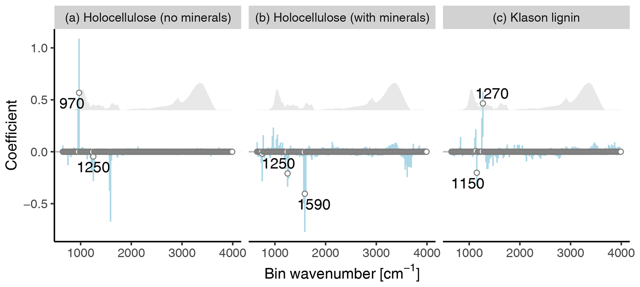
Figure 3Coefficients of the best models using binned spectra for holocellulose (a, b, model trained without and with samples containing minerals, respectively) and Klason lignin (c), plotted against the average wavenumber of the bins. Points are median coefficient estimates, error bars are 90 % posterior intervals. Points with an absolute median coefficient ≥0.2 are labeled with the respective average wavenumber value. The grey shaded region is a reference spectrum.
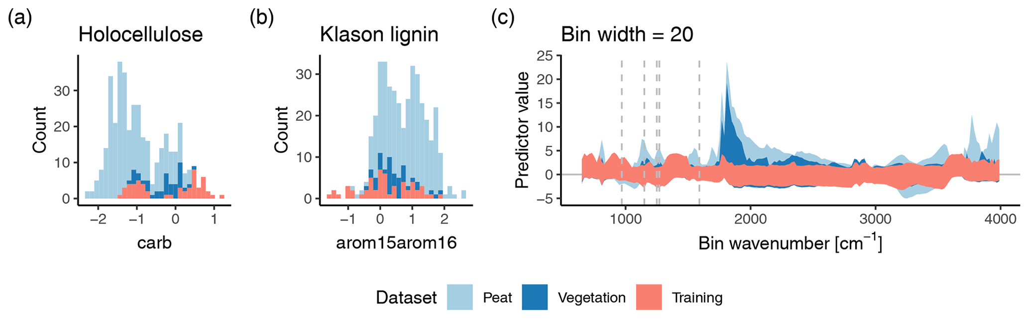
Figure 4Prediction domain for the original models (a, b) and the improved models using binned spectra with a bin width of 20 cm−1 (c). The prediction domain is the range of values covered by the predictor variables. The original models use only one predictor variable, and therefore the prediction domain can be shown as spread of the training samples across the x axis (standardized height of the carb and arom15arom16 peak, respectively) of a histogram (a, b; blue bars). Extrapolation occurs if other samples (peat, vegetation) exceed this range. Counts are number of samples in the respective datasets. The improved models include bins across the complete spectra (c). Therefore, the range in standardized predictor variable values (y axis) covered by the training data for each bin is shown as orange shaded area for the dataset with a bin width of 20 cm−1, as used by the (nearly) best improved models for holocellulose and Klason lignin. Extrapolation occurs if other samples (blue shaded regions) exceed these areas. Dashed lines indicate the most important variables for the holocellulose and Klason lignin model (compare with Fig. 3).
3.3 Is the prediction domain of the training data representative for peat samples?
The training data do not cover the range of the spectral variables relevant for predicting peat and peat-forming vegetation holocellulose contents (Fig. 4a and b). For the original models, the training data carb and arom15arom16 peak heights cover the range of the vegetation samples. However, few peat samples have larger arom15arom16 and many peat samples have smaller carb peak heights than covered by the training data. This suggests that the original models extrapolate holocellulose contents in peat samples with small holocellulose contents and also extrapolate Klason lignin contents in peat samples with large Klason lignin contents.
The same is true for the improved models using binned spectra (Fig. 4c). Even though it is not possible to establish a direct relation between extrapolation for individual spectral variables and predicted contents, it is visible that for several bins, peat samples, and – to a lesser extent – vegetation samples have mostly larger standardized predictor values than covered by the training data set. This is also true for bins with the largest absolute median coefficients (including the model for holocellulose fitted with mineral-rich samples; see Sect. 3.6 below).
Under what conditions does extrapolation occur? Samples with small carb peak, or for the binned spectra, large absorbance at ∼ 1250 and 1590 cm−1, are outside the prediction domain for holocellulose (Fig. 4). Since the carb peak is small and absorbance at the selected wavenumbers is typically large in decomposed samples (Cocozza et al., 2003; Tfaily et al., 2014; Hodgkins et al., 2018) (and the respective coefficients are negative), this indicates that for holocellulose, extrapolation occurs mainly for more decomposed peat.
This is also true for Klason lignin since extrapolation occurs for samples with large arom15arom16 peak, or for the binned spectra, large absorbance at ∼ 1150 and 1270 cm−1, all of which are larger for more decomposed peat (Cocozza et al., 2003; Tfaily et al., 2014; Hodgkins et al., 2018).
Overall, this indicates that the prediction domain formed by the training data does not cover the range needed for peat – particularly decomposed peat – and partly also does not cover the range needed for peat-forming vegetation samples. We assume that this is probably also true for non-peat SOM. Therefore the models' predictions can represent extrapolations in practice; the training data are not in general representative for peat and peat-forming vegetation.
Table 1Overview on the relative predictive performance of the models for holocellulose and Klason lignin content as measured using PSIS-LOO ELPD. For each variable, the model with the best average predictive performance (largest ELPD) is at the top and the other models follow in descending order. Models ending in “.2” and “.3” are the models with the original model structure as developed by Hodgkins et al. (2018). “Distribution” is the distribution assumed for the target variable. “Predictors” indicates if models were fitted with peaks extracted using the procedure of Hodgkins et al. (2018) (“peaks”) or using binned spectra (“bins”). “Prior” scale indicates the standard deviation for Gaussian coefficients (numeric values) or regularized horseshoe priors were used (“–”). “Bin width” is the width of bins (in wavenumber units). “ELPD” is the PSIS-LOO expected log-predictive density, ΔELPD the difference in ELPD relative to the average ELPD of the on-average best model, and ΔSE the standard error in the average ΔELPD.
3.4 How do predictions of the original and improved models differ?
There were considerable differences in predictions of the original and improved models using binned spectra for both Klason lignin and holocellulose for the peat samples (Figs. 5 and S5). For holocellulose, the original model tends to predict larger contents for peat, especially for samples with larger holocellulose contents (Fig. 5). Similar albeit less pronounced patterns are visible for the vegetation and training data. For Klason lignin, the improved model predicts up to 25 mass-% larger Klason lignin contents for some samples, but for others up to 10 mass-% smaller contents than the original model. This happens particularly in a region where the original model predicts Klason lignin contents between 25 and 35 mass-% (Fig. 5).
This is surprising for two reasons: first, for the training data, both models make quite similar predictions (Fig. 5). The peat samples have aro15arom16 values similar to the training data (Fig. 4), but nevertheless both models produce contrasting predictions. The same is true for holocellulose for a relatively large fraction of peat samples (Fig. 4). Second, both models have comparatively small bias within the range of the training data relevant to peat samples (Supplement Fig. S6). Thus, predictions are different for the peat samples even within the holocellulose and Klason lignin range covered by the training data, where the models actually make similar predictions for the training data. And these differences are not due to misfit of either model to the training data. This indicates that the spectra of the training data are not entirely representative for the peat samples, even if they are within the prediction domain (compare also with the previous section). What causes these differences?
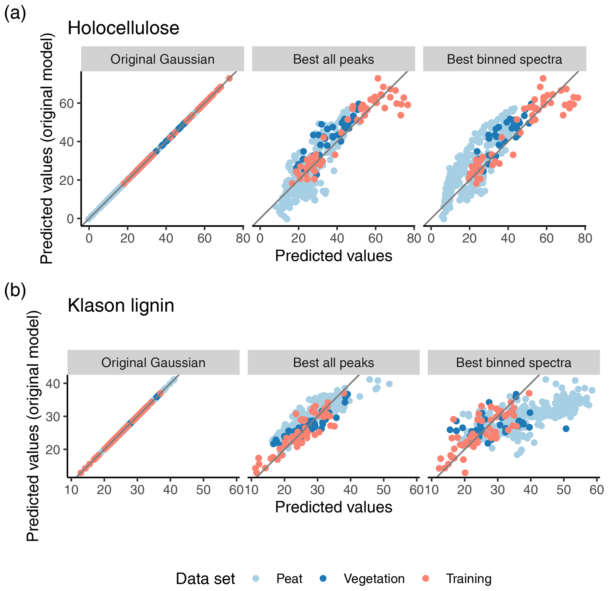
Figure 5Predicted values of the original model versus predicted values of the original model (first column), and the best improved models using extracted peaks (second column) and binned spectra (last column), respectively, for holocellulose (a) and Klason lignin (b), respectively. Colors differentiate the training, peat, and vegetation data from Hodgkins et al. (2018).
3.5 What causes differences in predictions?
We hypothesize that both the original and the improved models are not unbiased for samples with other spectral properties, even if these differences occur in variables not directly included in the models. For holocellulose, we could not find indications of which model is better. For Klason lignin, we provide mechanistic evidence for why the predictions of the improved models probably are more correct. Therefore, a key result of our analysis is that additional training and validation data are required to compute models to accurately predict SOM holocellulose and Klason lignin contents from MIRS.
3.5.1 Holocellulose
In comparison to the training data, spectra for peat typically have larger absorption values at around 1250 cm−1 and between (∼ 1250 to 1500 cm−1), but a smaller absorption in the region of the “OH peak” (∼ 3400 cm−1) (Supplement Fig. S13).
These spectral differences are directly related to the differences in predicted values of the original and improved model (Supplement Fig. S8): the smaller the OH peak is, the larger are predicted values of the original model in comparison to the improved model using binned spectra, especially for larger carb peak heights. Similarly, the larger the trough at 1250 cm−1 or the absorbance at 1590 cm−1 is, the larger are predictions of the original model in comparison to the improved model using binned spectra. This indicates that both the delineation of the carb peak and predictions using binned spectra are potentially sensitive to these differences and that this causes the observed differences in the predictions even in the range of the training data where both models yield similar predictions for the training samples.
What causes this sensitivity? Peak heights – for the original model – or spectral variables (bins) – for the improved models using binned spectra – are normalized by the sum of absorbance values in the complete spectra (Hodgkins et al., 2018). This is necessary to make spectra comparable, but also renders inferences sensitive to absorbance of other peaks not directly considered or with low influence in the original and improved models, respectively. Thus, if the OH peak is smaller, the normalized height of the carb peak is larger than for the same spectrum with a larger OH peak. Likewise, for the improved model using binned spectra a smaller OH peak results in larger absorbances around ∼ 1200 to 1600 cm−1 where the most influential variables are located (Supplement Figs. S7 and S2).
Why do peat samples have such different spectral properties? We hypothesize the following mechanistic explanation for the differences: decomposition of peat results in distinct changes in the absorbance at specific wavenumbers, e.g., the “OH peak” and the fingerprint region (e.g., Cocozza et al., 2003). For example, decomposition of phenols and disruption of tissue structures with hydrogen bonds result in a smaller absorbance around the OH peak (Kubo and Kadla, 2005; Schellekens et al., 2015). The training data contain only undecomposed or industrially processed OM (De la Cruz et al., 2016; Hodgkins et al., 2018) which do not reflect such decomposition changes and therefore generally have a larger OH peak (Supplement Fig. S7). For decomposed OM, the same normalized carb peak height or absorbance at specific wavenumbers therefore represents different holocellulose contents than for the training data, as the comparatively broad OH peak strongly influences the normalization of the spectra.
A consequence therefore is that it is questionable if the models (both original and improved) can be applied to peat and other SOM samples in general, without adapting the training data by including more representative samples.
3.5.2 Klason lignin
For Klason lignin, whereas the original model is unbiased across all samples (Supplement Fig. S6), it is not within two classes of training samples. Samples of these classes differ in the relative contribution of the arom15 and arom16 peaks to arom15arom16 (the sum of their heights) (Fig. 6). The first class (class 1) has high contributions of the arom15 peak (>30 %) and typically smaller arom15arom16 values; the second class (class 2) a smaller contribution of the arom15 peak and larger arom15arom16 values. Samples of both classes can have large or small actual Klason lignin contents (Fig. 6). What we observed is that the model makes biased predictions for both classes: for small arom15arom16 values, it underestimates contents, but for larger values, it increasingly overestimates Klason lignin contents (Supplement Fig. S9). For the improved model, this bias is much smaller (Figs. 6 and S9).
We suggest that it is this bias which causes most of the difference in predictions of the original and improved models. Conditional on the relative contribution of the arom15 peak to arom15arom16, peat samples have smaller and larger arom15arom16 values than the training data (Supplement Fig. S10). If one extrapolates the biased predictions of the original model for the training data classes, this means larger under- and overestimation for the peat samples than for the training data using the original model (Fig. 6). This is supported by measured peat Klason lignin contents: peat from temperate peatlands was reported to have Klason lignin contents as high as ∼ 70 mass-% and ∼ 57 mass-% on average (Hayes et al., 2015). Even though this was peat from extraction sites which probably is more decomposed (Hayes et al., 2015), this indicates that peat Klason lignin contents can be much larger, also in temperate regions, than predictions of the original model for wood-rich tropical peat (Hodgkins et al., 2018). In contrast, predictions under the improved model most probably reflect more correct Klason lignin estimates because the bias is much smaller and predicted values are larger for deeper peat samples. Therefore, this bias very likely is the reason why predictions of the original model differ from that of the improved model. Moreover, our results indicate that the improved model makes more correct predictions.
What causes this bias? We suggest that arom15arom16 is a poor indicator for Klason lignin content for samples with varying contents of proteins. Protein C-N and C=O stretching and N-H bending cause strong absorbance around 1560 and 1650 cm−1 (Stuart, 2004), and therefore it is not only aromatics which contribute to the arom16 peak. Larger arom16 peak heights may be indicative for Klason lignin, but can also be due to high protein contents.
This is what distinguishes samples of class 1 and 2 in the training data (Supplement Fig. S11): samples of class 1 are wood samples and paper product samples derived from wood. Wood typically has smaller nitrogen contents, but larger Klason lignin contents (Cowling and Merrill, 1966; Aerts et al., 1999; De la Cruz et al., 2016) which explains the large contribution of the arom15 peak, indicative for aromatic skeletal vibrations (but not for proteins) (Stuart, 2004) to arom15arom16. Conversely, samples of class 2 are leaf and needle samples which may contain both varying contents of Klason lignin and proteins (Aerts et al., 1999; Reich and Oleksyn, 2004; De la Cruz et al., 2016). Leaves and needles typically have larger protein contents than wood (Cowling and Merrill, 1966; Aerts et al., 1999; Reich and Oleksyn, 2004) and therefore a smaller contribution of the arom15 peak to arom15arom16. This is why the original model predicts high Klason lignin contents for samples of class 2, even though some of these actually have low Klason lignin contents (Fig. 6). The original model balances this, but in doing so it introduces the observed bias. As a consequence, arom15arom16 alone is a poor predictor for Klason lignin content of OM.
The improved model using binned spectra gives more weight to variables related to aromatic skeletal structures and not in a region where proteins cause large absorbances (Stuart, 2004) (Fig. 3). We suggest that these variables are better predictors for Klason lignin because they are interfered less by other molecular structures, such as proteins (Stuart, 2004). Overall, this mechanistic explanation provides additional evidence why the improved model using binned spectra probably makes more correct predictions.
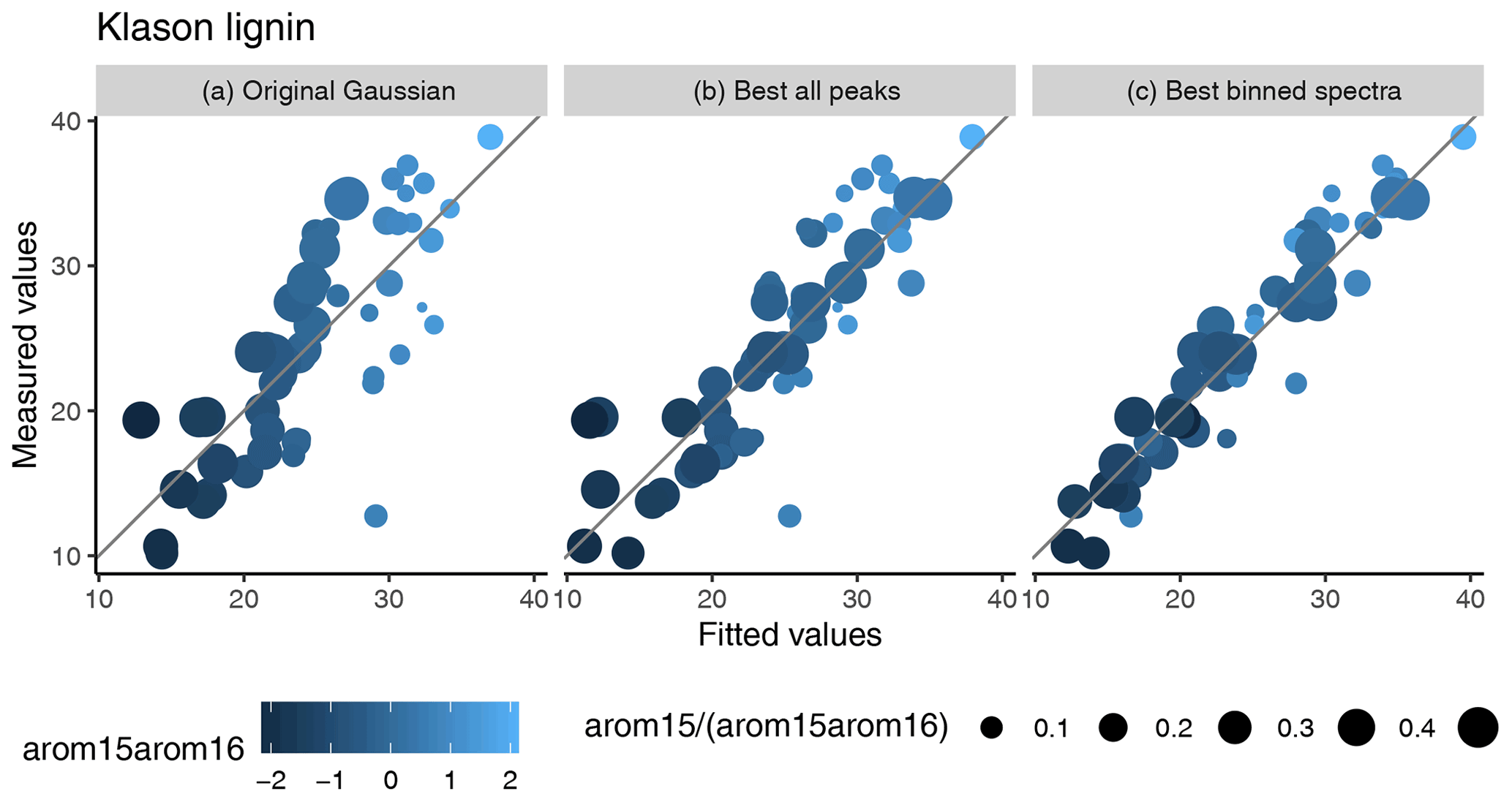
Figure 6Measured training data Klason lignin contents versus fitted values [mass-%] of the original model (a), the improved model using extracted peaks (b), and the improved model using binned spectra (c). Points are scaled according to the relative contribution of the arom15 peak to arom15arom16. The color gradient represents arom15arom16 values. The diagonal line represents values where measured and fitted values are identical.
3.6 Can holocellulose contents also be predicted for samples with mineral interferences?
Our analysis shows that models with similar fit to the training data can be computed also if mineral-rich samples are included. We see this as proof of concept that holocellulose contents can also be predicted from MIRS for SOM samples with mineral admixtures.
If the clay-rich old magazine samples are included, the model using binned spectra had the best average predictive performance. The model using extracted peaks had a worse but similar performance (, ΔSE=8.82). Moreover, the models trained on mineral-rich samples had a similar fit to the remaining samples as our improved models not trained with the mineral-rich samples (Supplement Fig. S12). In comparison to this, the original model considerably overestimated the holocellulose content for these samples, as observed by Hodgkins et al. (2018). This was also the case for the improved models not trained with the mineral rich samples (Supplement Fig. S12). We see this as proof of concept that it is possible to predict holocellulose contents from MIRS even for samples with high mineral contents. Moreover, there is no trade-off in predictive accuracy if mineral-rich samples are included, suggesting that general purpose models can be developed.
How do coefficients for the model trained with old magazine samples differ from the improved model trained without old magazine samples? According to Fig. 3 (middle panel), the “mineral-rich model” down-weights bins near the carb peak, in contrast to the improved model not trained on old magazine samples, and instead has a larger coefficient for an additional peak related to aromatic C=C stretching and amide N-H bending and C-N stretching (∼ 1590 cm−1) (Stuart, 2004) which corresponds to the arom15 peak. This provides further evidence that it is possible to infer holocellulose contents via aromatics.
3.7 General implications of our results
Our validation analysis provides general lessons for validating models using spectral data. What can we learn from the model validation? First, even though Hodgkins et al. (2018) had a sensible rationale in including only selected peaks into their models based upon causal knowledge, this strategy has critical weaknesses. If predictive accuracy is the main goal, pre-selecting variables triggers underfitting and bias and therefore is ineffective. Instead, it is more effective to include a larger set of variables in a model and to use regularization to avoid overfitting and find relations between predictor variables and the target variable (Piironen and Vehtari, 2017a).
Second, a linear relation between the target variable being predicted and a predictor variable is not sufficient validation of a spectral prediction model if the training data are not representative for the samples to which the model is applied. Most importantly, due to spectral normalization, predictions can be sensitive even to variables not included in the model. Therefore, to assess if training data (the prediction domain) are representative, whole spectra have to be compared.
Third, it is helpful to identify potential causal mechanisms which may affect differently the MIRS the model will be applied to than the MIRS it was trained on. As shown here (Sect. 3.5), differences in the degree of decomposition or the relative contribution of proteins and aromatic skeletal structures cause differences in MIRS which can result in biased predictions. Consequently, providing a causal explanation as to what causes the correlation between a target variable and specific MIRS variables is a useful tool to assess if a model may be applicable to new samples.
Fourth, our analysis also shows that re-evaluating existing models with their original training data can be an effective way to improve the models. Here, it was important that one modification of the original models often addressed multiple limitations at once due to interdependences between the limitations: improving the models' predictive performance did not only address underfitting, but also reduced the bias in the models (Fig. 6). Analyzing the prediction domain did not only show that the models extrapolate, but we could use this knowledge to analyze the practical impact of the bias. Lastly, including additional variables not only improved the predictive performance, but allowed us also to compute a model that probably is suitable for samples containing minerals. We therefore suggest that continuous re-evaluation of existing models can be an effective way to develop better models and should be part of a general model development workflow (Gelman et al., 2020).
There are several problems we could not solve. The most important problem is that also for the improved models, it is unclear if predictions are correct outside the prediction domain of the training data and therefore if the models are applicable to SOM in general.
Further issues are the following: (1) the overall accuracy of the models can certainly be improved with more training samples. (2) It is unclear how robust the original models and our improved models – especially models using binned spectra – are in terms of calibration transfer (calibration transfer is the application of a model to spectra measured differently than the training data, e.g., with a different procedure, on a different device, in a different laboratory Workman, 2018). We assume that the binning and estimation procedure are relatively robust since bin widths are comparatively broad and all variables were standardized, meaning that only between sample variability in intensities are relevant. However, this remains to be tested. (3) Even though we computed a model that could fit and predict mineral-rich samples, it is unclear whether this is possible in general. (4) Some of our models had computational issues (holocellulose: one model with maximally two divergent transitions, Klason lignin: two models with maximally five divergent transitions) that we could not resolve.
A further limitation is that, as the original models, the modified beta regression models do not consider the constraint that the contents of holocellulose, Klason lignin, and any remaining compounds should sum to 100 mass-%. This also represents a further test of how realistic model predictions are (compare with Sect. 2.1). In principle, this constraint could be considered by using a Dirichlet regression model (e.g., Douma and Weedon, 2019). We have not used this approach here due to higher computational costs, potential computational difficulties, keeping the present model validation straightforward, and since the training data do not fulfill this condition for all samples (Supplement Fig. S4; indicating that the measurement procedure needs to be improved too).
In summary, our analysis opens concrete and promising directions to further improve the models: we need training and validation data that include peat, particularly highly decomposed peat. Such data make it possible to analyze the impact of the bias and to compute models with less bias, higher representativity for SOM and peat, and potentially larger predictive accuracy. In addition to this, it is likely that an operative model for prediction of holocellulose contents in SOM samples with mineral admixtures can be developed by including such samples with more diverse minerals. Ideally, such improvements would be performed across multiple labs with an archive of sample materials such that calibration transfer of the models between different mid-infrared spectrometers can be further explored.
To support such developments, we implemented the best models using binned spectra (for holocellulose, the model which was also trained on mineral-rich samples) into the R package irpeat (Teickner and Hodgkins, 2020). The other models can be reproduced from the reproducible research compendium (Teickner and Knorr, 2022).
Our aim was to validate the original models of Hodgkins et al. (2018) to predict OM holocellulose and Klason lignin contents, identify weaknesses, provide a concrete strategy of how to tackle these problems, and provide first improvements using the same data.
The main weakness of the original models is the underlying training data: it is not in general representative for SOM, peat, and peat-forming vegetation. This results in biased predictions for holocellulose and Klason lignin for SOM, such as peat. Results from currently published studies using the original models should be interpreted with caution (we are currently preparing a manuscript, see Teickner and Knorr, 2022, which explores the implications of our results here for the results of Hodgkins et al., 2018). Manual variable selection favored this bias because it excluded information critical for better model fits. Finally, the original models can produce unrealistic (smaller than 0 or larger than 100 mass-%) predictions and prediction intervals.
Even though it was impossible to address the key problem of unrepresentative training data using the original data, we could address some of these issues, provide improved models, and develop a concrete strategy for future improvements. The improved models have less bias, avoid unrealistic predictions, and use information from the complete spectra and thus have a better predictive accuracy. Moreover, we provide a proof of concept that it is possible to predict holocellulose contents also for OM with mineral admixtures.
Our analysis thus opens concrete and promising directions to further improve the models: a major opportunity is to collect training and validation data representative for SOM, such that the improved models can be extended and thoroughly validated. In a next step, potential calibration transfer issues can be addressed.
Improved models to predict SOM holocellulose and Klason lignin contents can be of large importance in the long run because they allow cost-efficient high-throughput analyses of SOM. Detailed understanding of SOM chemistry across large scales, and the processes that result in changes in SOM chemistry, is only possible if such fast and effective tools are available.
The organic matter sample data from Hodgkins et al. (2018) as used to compute the models are available from the ir package (Teickner and Hodgkins, 2020). The peat and vegetation data from Hodgkins et al. (2018) analyzed in this study and the code to reproduce this paper are available from Teickner and Knorr (2022) and the development version via https://github.com/henningte/hklmirs (last access: 11 November 2022).
The supplement related to this article is available online at: https://doi.org/10.5194/soil-8-699-2022-supplement.
HT conceptualized the study, developed the methodology and software, and performed and validated the formal analysis, data curation, writing, and visualization. KHK supervised the study, provided the resources, acquired funding, and edited the manuscript.
The contact author has declared that neither of the authors has any competing interests.
Publisher’s note: Copernicus Publications remains neutral with regard to jurisdictional claims in published maps and institutional affiliations.
We would like to thank Hodgkins et al. (2018) and De la Cruz et al. (2016) for provision of data and code to reproduce and modify their analyses and Allaire et al. (2020) for provision of an Rmarkdown template. We thank Suzanne Hodgkins and Jeff Chanton for constructive discussions and Stephen Chapman and an anonymous reviewer for comments which helped to improve previous versions of this paper. We acknowledge support from the Open Access Publication Fund of the University of Münster.
This study was funded by the Deutsche Forschungsgemeinschaft (DFG) (grant no. KN 929/23-1 to Klaus-Holger Knorr and grant no. PE 1632/18-1 to Edzer Pebesma) and the Open Access Publication Fund of the University of Münster.
This paper was edited by Bas van Wesemael and reviewed by Stephen Chapman and one anonymous referee.
Aerts, R., Verhoeven, J. T. A., and Whigham, D. F.: Plant-Mediated Controls on Nutrient Cycling in Temperate Fens and Bogs, Ecology, 80, 2170–2181, https://doi.org/10.1890/0012-9658(1999)080[2170:PMCONC]2.0.CO;2, 1999. a, b, c
Ågren, G. I., Bosatta, E., and Agren, G. I.: Quality: A Bridge between Theory and Experiment in Soil Organic Matter Studies, Oikos, 76, 522–528, https://doi.org/10.2307/3546345, 1996. a
Allaire, J., Xie, Y., Wickham, H., Vaidyanathan, R., Boettiger, C., Broman, K., Mueller, K., Quast, B., Pruim, R., Marwick, B., Wickham, C., Keyes, O., Yu, M., Emaasit, D., Onkelinx, T., Gasparini, A., Desautels, M.-A., Leutnant, D., Öğreden, O., Hance, D., Nüst, D., Uvesten, P., Campitelli, E., Muschelli, J., Kamvar, Z. N., Ross, N., Cannoodt, R., Luguern, D., and Kaplan, D. M.: rticles: Article Formats for R Markdown, Version 0.14, CRAN, https://cran.r-project.org/web/packages/rticles/index.html (last access: 7 March 2022), 2020. a
Artz, R. R., Chapman, S. J., Jean Robertson, A., Potts, J. M., Laggoun-Défarge, F., Gogo, S., Comont, L., Disnar, J.-R., and Francez, A.-J.: FTIR Spectroscopy Can Be Used as a Screening Tool for Organic Matter Quality in Regenerating Cutover Peatlands, Soil Biol. Biochem., 40, 515–527, https://doi.org/10.1016/j.soilbio.2007.09.019, 2008. a
Bauer, I. E.: Modelling Effects of Litter Quality and Environment on Peat Accumulation over Different Time-Scales: Peat Accumulation over Different Time-Scales, J. Ecol., 92, 661–674, https://doi.org/10.1111/j.0022-0477.2004.00905.x, 2004. a
Baysinger, M. R., Wilson, R. M., Hanson, P. J., Kostka, J. E., and Chanton, J. P.: Compositional Stability of Peat in Ecosystem-Scale Warming Mesocosms, PLOS ONE, 17, e0263994, https://doi.org/10.1371/journal.pone.0263994, 2022. a
Bengtsson, F., Rydin, H., and Hájek, T.: Biochemical Determinants of Litter Quality in 15 Species of Sphagnum, Plant Soil, 425, 161–176, https://doi.org/10.1007/s11104-018-3579-8, 2018. a, b
Biester, H., Knorr, K.-H., Schellekens, J., Basler, A., and Hermanns, Y.-M.: Comparison of Different Methods to Determine the Degree of Peat Decomposition in Peat Bogs, Biogeosciences, 11, 2691–2707, https://doi.org/10.5194/bg-11-2691-2014, 2014. a, b, c
Bockheim, J. G.: Importance of Cryoturbation in Redistributing Organic Carbon in Permafrost-Affected Soils, Soil Sci. Soc. Am. J., 71, 1335–1342, https://doi.org/10.2136/sssaj2006.0414N, 2007. a
Broder, T., Blodau, C., Biester, H., and Knorr, K. H.: Peat Decomposition Records in Three Pristine Ombrotrophic Bogs in Southern Patagonia, Biogeosciences, 9, 1479–1491, https://doi.org/10.5194/bg-9-1479-2012, 2012. a
Bürkner, P.-C.: brms: An R Package for Bayesian Multilevel Models Using Stan, J. Stat. Softw., 80, 1–28, https://doi.org/10.18637/jss.v080.i01, 2017. a
Bürkner, P.-C.: Advanced Bayesian Multilevel Modeling with the R Package brms, R J., 10, 395–411, https://doi.org/10.32614/RJ-2018-017, 2018. a
Chen, C., Duan, C., Li, J., Liu, Y., Ma, X., Zheng, L., Stavik, J., and Ni, Y.: Cellulose (Dissolving Pulp) Manufacturing Processes and Properties: A Mini-Review, BioResources, 11, 5553–5564, https://doi.org/10.15376/biores.11.2.Chen, 2016. a
Cocozza, C., D'Orazio, V., Miano, T. M., and Shotyk, W.: Characterization of Solid and Aqueous Phases of a Peat Bog Profile Using Molecular Fluorescence Spectroscopy, ESR and FT-IR, and Comparison with Physical Properties, Organic Geochemistry, 34, 49–60, https://doi.org/10.1016/S0146-6380(02)00208-5, 2003. a, b, c, d
Cong, J., Gao, C., Han, D., Li, Y., and Wang, G.: Stability of the Permafrost Peatlands Carbon Pool under Climate Change and Wildfires during the Last 150 Years in the Northern Great Khingan Mountains, China, Sci. Total Environ., 712, 136476, https://doi.org/10.1016/j.scitotenv.2019.136476, 2020. a
Cong, J., Gao, C., Xing, W., Han, D., Li, Y., and Wang, G.: Historical Chemical Stability of Carbon Pool in Permafrost Peatlands in Northern Great Khingan Mountains (China) during the Last Millennium, and Its Paleoenvironmental Implications, CATENA, 209, 105853, https://doi.org/10.1016/j.catena.2021.105853, 2022. a
Cowling, E. B. and Merrill, W.: Nitrogen in Wood and Its Role in Wood Deterioration, Can. J. Bot., 44, 1539–1554, https://doi.org/10.1139/b66-167, 1966. a, b
De la Cruz, F. B., Osborne, J., and Barlaz, M. A.: Determination of Sources of Organic Matter in Solid Waste by Analysis of Phenolic Copper Oxide Oxidation Products of Lignin, J. Environ. Eng., 142, 04015076, https://doi.org/10.1061/(ASCE)EE.1943-7870.0001038, 2016. a, b, c, d, e, f, g, h, i
Douma, J. C. and Weedon, J. T.: Analysing Continuous Proportions in Ecology and Evolution: A Practical Introduction to Beta and Dirichlet Regression, Method. Ecol. Evol., 10, 1412–1430, https://doi.org/10.1111/2041-210X.13234, 2019. a
Elle, O., Richter, R., Vohland, M., and Weigelt, A.: Fine Root Lignin Content Is Well Predictable with Near-Infrared Spectroscopy, Sci. Rep., 9, 6396, https://doi.org/10.1038/s41598-019-42837-z, 2019. a, b, c
Gabry, J. and Mahr, T.: bayesplot: Plotting for Bayesian Models, CRAN, https://cran.r-project.org/web/packages/bayesplot/index.html (last access: 7 March 2022), 2020. a
Gelman, A., Vehtari, A., Simpson, D., Margossian, C. C., Carpenter, B., Yao, Y., Kennedy, L., Gabry, J., Bürkner, P.-C., and Modrák, M.: Bayesian Workflow, arXiv, arXiv:2011.01808 [stat], https://doi.org/10.48550/arXiv.2011.01808, 2020. a
Goodrich, B., Gabry, J., Ali, I., and Brilleman, S.: rstanarm: Bayesian Applied Regression Modeling via Stan, CRAN, https://cran.r-project.org/web/packages/rstanarm/index.html (last access: 7 March 2022), 2020. a, b
Harris, L. I., Moore, T. R., Roulet, N. T., and Pinsonneault, A. J.: Limited Effect of Drainage on Peat Properties, Porewater Chemistry, and Peat Decomposition Proxies in a Boreal Peatland, Biogeochemistry, 151, 43–62, https://doi.org/10.1007/s10533-020-00707-1, 2020. a
Hayes, D., Hayes, M., and Leahy, J.: Analysis of the Lignocellulosic Components of Peat Samples with Development of near Infrared Spectroscopy Models for Rapid Quantitative Predictions, Fuel, 150, 261–268, https://doi.org/10.1016/j.fuel.2015.01.094, 2015. a, b
Hodgkins, S. B., Richardson, C. J., Dommain, R., Wang, H., Glaser, P. H., Verbeke, B., Winkler, B. R., Cobb, A. R., Rich, V. I., Missilmani, M., Flanagan, N., Ho, M., Hoyt, A. M., Harvey, C. F., Vining, S. R., Hough, M. A., Moore, T. R., Richard, P. J. H., De La Cruz, F. B., Toufaily, J., Hamdan, R., Cooper, W. T., and Chanton, J. P.: Tropical Peatland Carbon Storage Linked to Global Latitudinal Trends in Peat Recalcitrance, Nat. Commun., 9, 3640, https://doi.org/10.1038/s41467-018-06050-2, 2018. a, b, c, d, e, f, g, h, i, j, k, l, m, n, o, p, q, r, s, t, u, v, w, x, y, z, aa, ab, ac, ad, ae, af, ag, ah, ai, aj, ak, al, am, an, ao, ap, aq, ar, as, at, au, av, aw, ax, ay
Koven, C., Friedlingstein, P., Ciais, P., Khvorostyanov, D., Krinner, G., and Tarnocai, C.: On the Formation of High-Latitude Soil Carbon Stocks: Effects of Cryoturbation and Insulation by Organic Matter in a Land Surface Model, Geophys. Res. Lett., 36, L21501, https://doi.org/10.1029/2009GL040150, 2009. a
Kubo, S. and Kadla, J. F.: Hydrogen Bonding in Lignin: A Fourier Transform Infrared Model Compound Study, Biomacromolecules, 6, 2815–2821, https://doi.org/10.1021/bm050288q, 2005. a, b, c
Lehmann, J. and Kleber, M.: The Contentious Nature of Soil Organic Matter, Nature, 528, 60–68, https://doi.org/10.1038/nature16069, 2015. a
Leifeld, J., Steffens, M., and Galego-Sala, A.: Sensitivity of Peatland Carbon Loss to Organic Matter Quality, Geophys. Res. Lett., 39, L14704, https://doi.org/10.1029/2012GL051856, 2012. a, b
Loisel, J., Yu, Z., Beilman, D. W., Camill, P., Alm, J., Amesbury, M. J., Anderson, D., Andersson, S., Bochicchio, C., Barber, K., Belyea, L. R., Bunbury, J., Chambers, F. M., Charman, D. J., De Vleeschouwer, F., Fiałkiewicz-Kozieł, B., Finkelstein, S. A., Gałka, M., Garneau, M., Hammarlund, D., Hinchcliffe, W., Holmquist, J., Hughes, P., Jones, M. C., Klein, E. S., Kokfelt, U., Korhola, A., Kuhry, P., Lamarre, A., Lamentowicz, M., Large, D., Lavoie, M., MacDonald, G., Magnan, G., Mäkilä, M., Mallon, G., Mathijssen, P., Mauquoy, D., McCarroll, J., Moore, T. R., Nichols, J., O'Reilly, B., Oksanen, P., Packalen, M., Peteet, D., Richard, P. J., Robinson, S., Ronkainen, T., Rundgren, M., Sannel, A. B. K., Tarnocai, C., Thom, T., Tuittila, E.-S., Turetsky, M., Väliranta, M., van der Linden, M., van Geel, B., van Bellen, S., Vitt, D., Zhao, Y., and Zhou, W.: A Database and Synthesis of Northern Peatland Soil Properties and Holocene Carbon and Nitrogen Accumulation, The Holocene, 24, 1028–1042, https://doi.org/10.1177/0959683614538073, 2014. a
Moore, T. R., Knorr, K.-H., Thompson, L., Roy, C., and Bubier, J. L.: The Effect of Long-Term Fertilization on Peat in an Ombrotrophic Bog, Geoderma, 343, 176–186, https://doi.org/10.1016/j.geoderma.2019.02.034, 2019. a
Peltre, C., Thuriès, L., Barthès, B., Brunet, D., Morvan, T., Nicolardot, B., Parnaudeau, V., and Houot, S.: Near Infrared Reflectance Spectroscopy: A Tool to Characterize the Composition of Different Types of Exogenous Organic Matter and Their Behaviour in Soil, Soil Biol. Biochem., 43, 197–205, https://doi.org/10.1016/j.soilbio.2010.09.036, 2011. a
Piironen, J. and Vehtari, A.: Comparison of Bayesian Predictive Methods for Model Selection, Stat. Comput., 27, 711–735, https://doi.org/10.1007/s11222-016-9649-y, 2017a. a, b
Piironen, J. and Vehtari, A.: On the Hyperprior Choice for the Global Shrinkage Parameter in the Horseshoe Prior, arXiv, arXiv:1610.05559 [stat], https://doi.org/10.48550/arXiv.1610.05559, 2017b. a
Piironen, J., Paasiniemi, M., and Vehtari, A.: Projective Inference in High-Dimensional Problems: Prediction and Feature Selection, Electron. J. Stat., 14, 2155–2197, https://doi.org/10.1214/20-EJS1711, 2020. a
Piñeiro, G., Perelman, S., Guerschman, J. P., and Paruelo, J. M.: How to Evaluate Models: Observed vs. Predicted or Predicted vs. Observed?, Ecol. Model., 216, 316–322, https://doi.org/10.1016/j.ecolmodel.2008.05.006, 2008. a
R Core Team: R: A Language and Environment for Statistical Computing, R Foundation for Statistical Computing, Vienna, Austria, https://www.r-project.org/ (last access: 7 March 2022), 2020. a
Raftery, A. E. and Zheng, Y.: Discussion: Performance of Bayesian Model Averaging, J. Am. Stat. Assoc., 98, 931–938, https://doi.org/10.1198/016214503000000891, 2003. a
Reich, P. B. and Oleksyn, J.: Global Patterns of Plant Leaf N and P in Relation to Temperature and Latitude, P. Natl. Acad. Sci. USA, 101, 11001–11006, https://doi.org/10.1073/pnas.0403588101, 2004. a, b
Scharlemann, J. P., Tanner, E. V., Hiederer, R., and Kapos, V.: Global Soil Carbon: Understanding and Managing the Largest Terrestrial Carbon Pool, Carbon Manag., 5, 81–91, https://doi.org/10.4155/cmt.13.77, 2014. a
Schellekens, J., Bindler, R., Martínez-Cortizas, A., McClymont, E. L., Abbott, G. D., Biester, H., Pontevedra-Pombal, X., and Buurman, P.: Preferential Degradation of Polyphenols from Sphagnum – 4-Isopropenylphenol as a Proxy for Past Hydrological Conditions in Sphagnum-dominated Peat, Geochim. Cosmochim. Ac., 150, 74–89, https://doi.org/10.1016/j.gca.2014.12.003, 2015. a
Shipley, B. and Tardif, A.: Causal Hypotheses Accounting for Correlations between Decomposition Rates of Different Mass Fractions of Leaf Litter, Ecology, 102, e03196, https://doi.org/10.1002/ecy.3196, 2021. a, b
Stan Development Team: RStan: The R Interface to Stan, 2020. a
Stan Development Team: Stan Modeling Language Users Guide and Reference Manual, Stan Development Team, https://mc-stan.org/docs/stan-users-guide/index.html (last access: 11 November 2022), 2021. a
Stuart, B. H.: Infrared Spectroscopy: Fundamentals and Applications, Analytical Techniques in the Sciences, John Wiley & Sons, Ltd, Chichester, UK, https://doi.org/10.1002/0470011149, 2004. a, b, c, d, e, f, g, h
Sun, B., Liu, J., Liu, S., and Yang, Q.: Application of FT-NIR-DR and FT-IR-ATR Spectroscopy to Estimate the Chemical Composition of Bamboo (Neosinocalamus Affinis Keng), Holzforschung, 65, 689–696, https://doi.org/10.1515/hf.2011.075, 2011. a
Teickner, H.: ir: A Simple Package to Handle and Preprocess Infrared Spectra, Zenodo [code], https://doi.org/10.5281/zenodo.5747170, 2020. a
Teickner, H. and Hodgkins, S. B.: irpeat: Simple Functions to Analyse Mid Infrared Spectra of Peat Samples, Zenodo [code], https://doi.org/10.5281/zenodo.7262744, 2020. a, b, c, d
Teickner, H. and Knorr, K.-H.: hklmirs: Reproducible Research Compendium for “Improving Models to Predict Holocellulose and Klason Lignin Contents for Peat Soil Organic Matter with Mid Infrared Spectra” and “Comment on Hodgkins et al. (2018): Predicting Absolute Holocellulose and Klason Lignin Contents for Peat Remains Challenging” (v0.2.0), Zenodo [code], https://doi.org/10.5281/zenodo.7255108, 2022. a, b, c
Teickner, H., Estop-Aragonés, C., and Zając, K.: Elevated Nitrogen Deposition Resulted in Enhanced Peat Decomposition Across Europe During the 20th Century, Tech. rep., 36, EGU2019-5778, 2019. a
Teickner, H., Gao, C., and Knorr, K.-H.: Electrochemical Properties of Peat Particulate Organic Matter on a Global Scale: Relation to Peat Chemistry and Degree of Decomposition, Global Biogeochem. Cy., 36, e2021GB007160, https://doi.org/10.1029/2021GB007160, 2022. a, b
Tfaily, M. M., Cooper, W. T., Kostka, J. E., Chanton, P. R., Schadt, C. W., Hanson, P. J., Iversen, C. M., and Chanton, J. P.: Organic Matter Transformation in the Peat Column at Marcell Experimental Forest: Humification and Vertical Stratification: Organic Matter Dynamics, J. Geophys. Res.-Biogeo., 119, 661–675, https://doi.org/10.1002/2013JG002492, 2014. a, b
Vehtari, A., Gelman, A., and Gabry, J.: Practical Bayesian Model Evaluation Using Leave-One-out Cross-Validation and WAIC, Stat. Comput., 27, 1413–1432, https://doi.org/10.1007/s11222-016-9696-4, 2017. a, b, c, d, e
Vehtari, A., Gabry, J., Magnusson, M., Yao, Y., Bürkner, P.-C., Paananen, T., Gelman, A., Goodrich, B., and Piironen, J.: loo: Efficient Leave-One-out Cross-Validation and WAIC for Bayesian Models, CRAN, https://cran.r-project.org/web/packages/loo/index.html (last access: 7 March 2022), 2019. a, b, c
Verbeke, B. A., Lamit, L. J., Lilleskov, E. A., Hodgkins, S. B., Basiliko, N., Kane, E. S., Andersen, R., Artz, R. R. E., Benavides, J. C., Benscoter, B. W., Borken, W., Bragazza, L., Brandt, S. M., Bräuer, S. L., Carson, M. A., Charman, D., Chen, X., Clarkson, B. R., Cobb, A. R., Convey, P., Águila Pasquel, J., Enriquez, A. S., Griffiths, H., Grover, S. P., Harvey, C. F., Harris, L., Hazard, C., Hodgson, D., Hoyt, A. M., Hribljan, J., Jauhiainen, J., Juutinen, S., Knorr, K.-H., Kolka, R. K., Könönen, M. T., Larmola, T., McCalley, C. K., McLaughlin, J., Moore, T. R., Mykytczuk, N., Normand, A. E., Rich, V., Roulet, N., Royles, J., Rutherford, J., Smith, D. S., Svenning, M. M., Tedersoo, L., Thu, P. Q., Trettin, C. C., Tuittila, E.-S., Urbanová, Z., Varner, R. K., Wang, M., Wang, Z., Warren, M., Wiedermann, M. M., Williams, S., Yavitt, J. B., Yu, Z.-G., Yu, Z., and Chanton, J. P.: Latitude, Elevation, and Mean Annual Temperature Predict Peat Organic Matter Chemistry at a Global Scale, Global Biogeochem. Cy., 36, e2021GB007057, https://doi.org/10.1029/2021GB007057, 2022. a
Viscarra Rossel, R., Walvoort, D., McBratney, A., Janik, L., and Skjemstad, J.: Visible, near Infrared, Mid Infrared or Combined Diffuse Reflectance Spectroscopy for Simultaneous Assessment of Various Soil Properties, Geoderma, 131, 59–75, https://doi.org/10.1016/j.geoderma.2005.03.007, 2006. a
Wadoux, A. M.-C., Malone, B., Minasny, B., Fajardo, M., and McBratney, A. B.: Soil Spectral Inference with R: Analysing Digital Soil Spectra Using the R Programming Environment, Progress in Soil Science, Springer International Publishing, Cham, ISBN 978-3-030-64896-1, https://doi.org/10.1007/978-3-030-64896-1, 2021. a, b, c, d
Workman, J. J.: A Review of Calibration Transfer Practices and Instrument Differences in Spectroscopy, Appl. Spectros., 72, 340–365, https://doi.org/10.1177/0003702817736064, 2018. a
Worrall, F., Moody, C. S., Clay, G. D., Burt, T. P., and Rose, R.: The Flux of Organic Matter through a Peatland Ecosystem: The Role of Cellulose, Lignin, and Their Control of the Ecosystem Oxidation State: Flux of Organic Matter Through a Peat, J. Geophys. Res.-Biogeo., 122, 1655–1671, https://doi.org/10.1002/2016JG003697, 2017. a
Xiaobo, Z., Jiewen, Z., Povey, M. J., Holmes, M., and Hanpin, M.: Variables Selection Methods in Near-Infrared Spectroscopy, Anal. Chim. Ac., 667, 14–32, https://doi.org/10.1016/j.aca.2010.03.048, 2010. a, b