the Creative Commons Attribution 4.0 License.
the Creative Commons Attribution 4.0 License.
 | 22 Jan 2021
Mapping soil slaking index and assessing the impact of management in a mixed agricultural landscape
Edward J. Jones
Patrick Filippi
Rémi Wittig
Mario Fajardo
Vanessa Pino
Alex B. McBratney
Soil aggregate stability is a useful indicator of soil physical health and can be used to monitor condition through time. A novel method of quantifying soil aggregate stability, based on the relative increase in the footprint area of aggregates as they disintegrate when immersed in water, has been developed and can be performed using a smartphone application – SLAKES. In this study the SLAKES application was used to obtain slaking index (SI) values of topsoil samples (0 to 10 cm) at 158 sites to assess aggregate stability in a mixed agricultural landscape. A large range in SI values of 0 to 7.3 was observed. Soil properties and land use were found to be correlated with observed SI values. Soils with clay content >25 % and cation exchange capacity (CEC) : clay ratio >0.5 had the highest observed SI values. Variation in SI for these soils was driven by organic carbon (OC) content which fit a segmented exponential decay function. An OC threshold of 1.1 % was observed, below which the most extreme SI values were observed. Soils under dryland and irrigated cropping had lower OC content and higher observed SI values compared to soils under perennial cover. These results suggest that farm managers can mitigate the effects of extreme slaking by implementing management practices to increase OC content, such as minimum tillage or cover cropping. A regression-kriging method utilising a Cubist model with a suite of spatial covariates was used to map SI across the study area. Accurate predictions were produced with leave-one-out cross-validation, giving a Lin's concordance correlation coefficient (LCCC) of 0.85 and a root-mean-square error (RMSE) of 1.1. Similar validation metrics were observed in an independent test set of samples consisting of 50 observations (LCCC = 0.82; RMSE = 1.1). The potential impact of implementing management practices that promote soil OC sequestration on SI values in the study area was explored by simulating how a 0.5 and 1.0 % increase in OC would impact SI values at observation points and then mapping this across the study area. Overall, the maps produced in this study have the potential to guide management decisions by identifying areas that currently experience extreme slaking and highlighting areas that are expected to have a significant reduction in slaking by increasing OC content.
- Article
(2303 KB) - Full-text XML
- BibTeX
- EndNote


Objective and quantitative metrics are required to assess soil health and monitor soil condition through time. Development of simple accessible metrics to assess soil health will facilitate increased spatial and temporal sampling density, and will encourage farmers, consultants, and even citizens to participate in soil health assessment. Aggregate stability is an important indicator of physical condition that quantifies a soil's resistance to slaking and dispersion. Slaking is the disintegration of soil aggregates as a result of rapid wetting (Yoder, 1936; Oades and Waters, 1991). Slaking occurs when soil aggregates are unable to withstand the stress induced by water uptake derived from two main causes: swelling of clay minerals as water is adsorbed into the interstitial space and internal pressure caused by compression of entrapped air bubbles as capillary action draws water into the small pores between soil particles (Emerson, 1964). Most cultivated soils in Australia are prone to some degree of slaking. The degree of slaking determines if the process produces a favourable or unfavourable environment for cultivation and plant growth, and it has implications for soil conservation. A small degree of slaking can be beneficial and is associated with self-mulching – an ability to recover from disturbance by reforming small (<5 mm) aggregates at the soil surface following wetting–drying cycles (Grant and Blackmore, 1991) – and mellowing: a partial disintegration of soil aggregates on wetting that results in increased friability (Barzegar et al., 1996). Slaking produces detrimental effects when aggregates disintegrate further into microaggregates (∅ <0.25 mm). Detached microaggregates migrate and settle into pores, reducing pore volume, decreasing infiltration and percolation rates, and leading to increased surface run-off (Rengasamy et al., 1984). Erosion susceptibility is exacerbated as greater run-off volumes increase erosive power, and the slaked aggregates also provide suitably sized particles for translocation. Ultimately the soil has a lowered capacity to support plant growth as plant-available water and soil–atmosphere gas exchange are both reduced. In severe cases, crusting or hard setting occurs when slaked and dispersed aggregates coalesce and set hard on drying (Mullins et al., 1990). Soil strength increases as the soil dries, producing difficulty in cultivation until the soil is rewetted, and shoot emergence and root growth may be restricted (Mullins et al., 1990).
The susceptibility of a soil aggregate to slake is related to texture, mineral composition, and organic matter content (Mullins et al., 1990). Soils with high clay content, especially those containing smectite or vermiculite minerals, are more likely to slake as they expand on wetting and also contain a greater number of small diameter pores into which capillary action will draw water and compress entrapped air bubbles (Emerson, 1964). High organic matter content improves soil structure by binding soil particles into stable aggregates and reducing susceptibility to slaking (Chenu et al., 2000). Techniques that increase soil organic matter – such as cover cropping, reduced tillage, and application of organic amendments – may reduce susceptibility to slaking. Agricultural management practices that increase susceptibility to slaking include conventional tillage methods that destroy soil structure and accelerate organic matter decomposition, burning or removal of crop residues, and the application of pesticides and other chemicals that are harmful to soil biota and lead to disruption of organic matter cycling and reduced aggregation. The detrimental effects of soil slaking are more pronounced in areas with clear wetting–drying cycles, such as temperate Australia. Collis-George and Lal (1971) found that the initial water content of soil affects the degree of slaking upon rewetting, and soils of low initial water content are more prone to rapid and explosive slaking.
Slaking and dispersion are quantified through aggregate stability tests that observe changes in soil aggregate morphology following immersion in water in an attempt to predict soil behaviour in the field. Emerson (1967) developed a test to classify samples into eight classes based on the degree of slaking, swelling, and dispersion observed when air-dried soil aggregates are immersed in distilled water. The Emerson aggregate test was extended by including a supplementary analysis whereby soil samples were wetted and moulded into cubes before immersion in the distilled water as a means to simulate the shear forces associated with raindrop impact and tillage on bare soil (Loveday and Pyle, 1973; Emerson, 1991). Field et al. (1997) modified these tests further to include observations of slaking and dispersion at both 10 min and 2 h post-submersion in the “aggregate stability in water” (ASWAT) test. This greatly decreased the time requirement from 20+ h required for previous tests; however, interpretation of the degree of slaking for the ASWAT test remained moderately subjective, and scores were produced on an ordinal scale from 0 to 4, which limits statistical applications. Established methods of quantifying stability of aggregates subject to wet sieving or simulated rainfall are also time-consuming and require specialist equipment (Yoder, 1936; Schindelbeck et al., 2016).
A new method has been developed to calculate degree of slaking using a time series of digital photographs to quantify the increase of the footprint area of aggregates as they disintegrate when immersed in distilled water (Fajardo et al., 2016). This method has been incorporated into a smartphone application, SLAKES, that is able to quantify aggregate stability in only 10 min (Fajardo and McBratney, 2019). The reduced assessment time was achieved as the authors found that the 2 h reading can be reliably estimated from change in footprint area over the 10 min analysis period. The SLAKES application requires no specialty equipment, and the automated nature of the application allows aggregate stability to be quantified with minimal training. These advances make the analysis more readily available to farm managers and citizen scientists. The method calculates an objective and continuous slaking index (SI), which reduces operator error and facilitates elucidation of contributing factors of observed slaking. For example, Flynn et al. (2020) investigated aggregate stability of Vertisols under different agricultural management strategies and found that SI was significantly more sensitive at distinguishing the perennial, no-till, and conventional tillage management treatments compared to the Cornell wet aggregate stability test (Schindelbeck et al., 2016).
Few studies have mapped aspects of soil aggregate stability using digital soil mapping (DSM) techniques. Odeh and Onus (2008) used regression kriging and indicator kriging to model the electrochemical stability index (ESI) across an irrigated cropping region of western NSW, Australia. This resulted in a map of “risk zones” that were susceptible to dispersion and that could be prioritised for increased monitoring and tactical management to abate immediate and future detrimental impacts on crop production. A study by Annabi et al. (2017) also utilised regression kriging to produce accurate predictions of soil aggregate stability of an agricultural district in Tunisia. Fine-resolution maps of soil aggregate stability across fields and farms have considerable potential to aid farm managers in decision-making processes. Such maps could guide farm managers to implement soil amelioration practices, such as tactical application of gypsum, or change in management practices, such as minimum tillage or use of cover crops. Tools that make aggregate stability quantification accessible, such as the SLAKES application, may facilitate the production of such maps.
The current study investigated the use of the SLAKES application and DSM techniques to assess variation in SI across a landscape with different agricultural and natural land uses. The contribution of both soil attributes and land management to slaking was investigated, and the potential impact of increasing soil organic carbon (OC) levels on slaking was explored.
2.1 Site description
The study was centred around a mixed farming property, L'lara (30∘15′18′′ S, 149∘51′39′′ E), which is located ∼ 11 km north-east of the township of Narrabri, NSW, Australia (Fig. 1). Climate at the study site is classified as humid subtropical (Cfa) under the Köppen–Geiger system (Peel et al., 2007). The site experiences hot summers and cool winters. The long-term average annual precipitation for the study area is 658 mm and is slightly summer-dominant (Bureau of Meteorology, 2020). The landscape at L'lara and its surrounds can be broadly characterised into two distinct areas: sand-covered hills derived predominantly from Jurassic coarse-grained sediments of Pilliga sandstone covered by Quaternary sands and talus material, and floodplain areas derived from Quaternary alluvial deposits of basaltic materials washed from the western side of the Nandewar range. The soils of the floodplain area at L'lara are classified as Vertisols according to the World Reference Base for Soil Resources, with some expression of calcic horizons (IUSS Working Group WRB, 2014). The sand hill area is represented by Luvisol, Lixisol, Solonetz, Leptosol, and Regosol soil groups. L'lara encompasses a total area of 1850 ha, with approximately 1070 ha used for dryland cropping. Cropping is performed primarily on the Vertisols and occurs over both summer and winter periods with cotton (Gossypium hirsutum L.), wheat (Triticum aestivum L.), canola (Brassica napus L.), and chickpea (Cicer arietinum L.) grown in rotation. Lower-lying floodplain areas close to creek lines and all of the sand hill area are used for grazing of beef cattle on unimproved native pastures (∼ 704 ha) and remnant forest cover (∼ 76 ha).
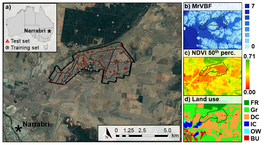
Figure 1(a) Location of L'lara farm and the wider study area in relation to the township of Narrabri, NSW, Australia. Sample locations used as a training set (n = 108) and test set (n = 50) are indicated. Satellite imagery sourced from Google Earth Pro V 7.3.2.5776 (5 March 2019). Narrabri, NSW, Australia. 30∘16′31.37′′ S, 149∘51′46.42′′ E. Eye altitude: 20.57 km. Image © CNES/Airbus 2020 (http://www.earth.google.com, last access: 20 April 2020). (b) MrVBF calculated at 30 m resolution using the SRTM digital elevation model. (c) Pixel-wise 50th percentile of NDVI calculated from Landsat 7 scenes covering the time period 2000 to 2018. (d) Simplified land use across the study area (ABARES, 2018). FR: forest reserve; Gr: grazing including understorey grazing and stock routes; DC: dryland cropping; IC: irrigated cropping; OW: open water; BU: built-up areas. The external perimeter boundary of L'lara is indicated by the thick black line, and boundaries of cropping paddocks are indicated by thin black lines.
L'lara lies at the centre of a diverse landscape. Outside the property, dryland cropping and grazing occur on the floodplains and slopes to the east and south. Intensive irrigated agricultural production occurs on the lower floodplain to the south-west of the property, and the Killarney State Conservation Area lies directly to the north. This conservation area contains similar species to the remnant forest area found at L'lara, which is dominated by white cypress pine (Callitris glaucophylla), hickory (Acacia leiocalyx), black cypress pine (Callitris endlicheri), narrow-leaved ironbark (Eucalyptus crebra), bull oak (Allocasuarina luehmannii), and dirty gum (Eucalyptus chloroclada).
2.2 Soil sampling
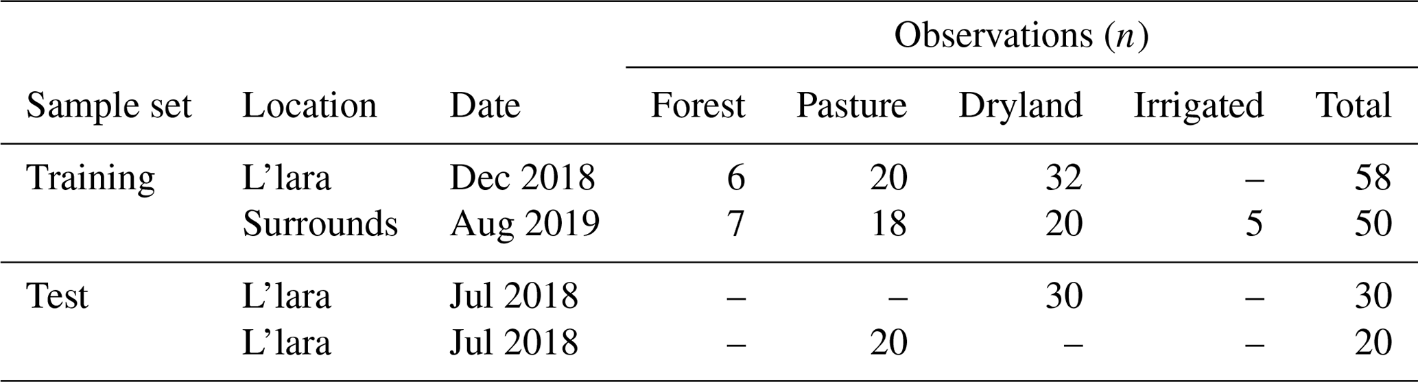
A training set of 108 samples and a test set of 50 samples were defined (Table 1). The training set comprised both on- and off-farm samples. The on-farm samples (n = 58) were identified based on a random stratified sampling approach utilising soil type and land use as parameters (Fig. 1). This ensured representation of the major soil types and different land uses – dryland cropping, pasture, and forest cover found on the property. The off-farm samples (n = 50) samples were sourced from neighbouring properties found within a 5 km distance from the boundary of L'lara. As a soil type map was not available for off-farm locations, the sites were identified through a random stratified approach utilising k-means clustering and rasters of elevation, multi-resolution valley bottom flatness (MrVBF), and airborne gamma radiometrics as input variables (Filippi et al., 2020). Four strata were identified whose geographic distribution was approximately equivalent to sand hill, transition, upper floodplain, and lower floodplain landscape positions. Sample sites were randomly selected within each stratum. Five of the samples on the lower floodplain were under irrigated agriculture, a land use not represented at L'lara. The test set was constructed utilising 30 existing sites in the dryland cropping areas of L'lara, which are described in Filippi et al. (2019), and 20 sites in the pasture areas. At each of the 158 sites a topsoil (0 to 10 cm) sample was obtained by excavation using a shovel at a discrete location.
Table 1Summary of sampling campaigns and land use for each dataset.
2.3 Sample preparation and laboratory methods
All soil samples were air-dried at 40 ∘C for 48 h. A selection of 12 to 15 soil aggregates (∅ 5–10 mm) were isolated from the air-dried bulk soil samples prior to grinding and sieving for laboratory analysis. If distinct aggregates were not immediately evident in the bulk soil, then the sample was passed through a 5 mm sieve to isolate aggregates; this procedure was often required in sandy soils. The remaining sample was then ground to pass through a 2 mm sieve prior to laboratory analysis. Particle size analysis was performed using the hydrometer method (Gee and Bauder, 1986). Organic carbon content was quantified using the Walkley–Black method (Walkley and Black, 1934). Soil pH and electrical conductivity (EC) were measured using a 1:5 soil / H2O suspension. As the soil samples did not contain significant quantities of carbonates or soluble salts, the cation exchange capacity (CEC) was assessed using the ammonium acetate method (Rayment and Lyons, 2011). Exchangeable sodium percentage (ESP) and Ca : Mg ratio were calculated from the relevant exchangeable cations, and the CEC : clay ratio was calculated following correction for the CEC contribution of organic matter. Laboratory data were obtained on the 108 samples of the training set only; for the test set only slaking index information was obtained.
2.4 SLAKES slaking index
A slaking index (SI) was obtained using the SLAKES application (Fajardo and McBratney, 2019). Briefly, a smartphone (Galaxy J2 Pro, Samsung, Republic of Korea) with an 8 MP digital camera was fixed on an articulated stand to provide the camera lens an unimpeded view of the bench surface. The height of the stand was adjusted so that the field of view of the camera was filled by a 100 mm diameter Petri dish placed on the surface of the bench directly below the camera. Three soil aggregates were placed into the Petri dish, and an initial image of the aggregates was acquired. The Petri dish was then drawn back and replaced by an identical Petri dish filled with sufficient deionised water to completely immerse the aggregates. The aggregates were held directly above the deionised water and dropped simultaneously into the Petri dish, with care being taken to preserve the order and orientation of the aggregates to that of the initial image. The start button of the SLAKES application was then immediately pressed, and the set-up left to process over a 10 min period, after which the SI was displayed on the screen of the smartphone. The experiment was performed on a white surface to increase contrast between the soil aggregates and the background surface. The experiment was also performed under diffuse and constant lighting to prevent the occurrence of shadows over the Petri dish, which could introduce errors during the image segmentation process. The procedure was repeated twice for each sample; if the difference between the duplicate readings was greater than one unit, an additional reading was obtained. An additional reading was required for approximately 20 % of samples and was more commonly required for soils with higher slaking index values compared to samples which exhibited minimal slaking. When additional readings were taken, the outlier reading was discarded and remaining readings averaged to provide the final SI for each sample.
The SLAKES application uses an image segmentation approach to calculate the footprint area of each aggregate, expressed as pixel count, and tracks the relative increase in area of individual aggregates as they break down over time (Fajardo et al., 2016). The SI of an individual aggregate at a given time after immersion is calculated as
where A0 is the initial footprint area of the aggregate and At is the footprint area of the aggregate at time t. An SI of 0 means that the footprint area of the aggregate has not increased at all, an SI of 1 means that the footprint area has increased in size by 100 %, an SI of 2 means that the footprint area has increased in size by 200 %, etc. The change in SI over the course of the analysis is used to fit a Gompertz function on a log timescale and calculate parameters a, b, and c:
where, as described in Fajardo et al. (2016), a is an asymptote representing the maximum SI after an indefinite period of time, b describes displacement along the time axis and is associated with initial slaking, and c describes the growth rate and is associated with ongoing slaking of the aggregate. The SI value returned from the SLAKES application is the average of the a parameter calculated individually for each aggregate. A major benefit of this approach is that this value can be estimated after only 10 min of immersion, unlike the ASWAT test, which requires 2 h of immersion.
2.5 Spatial covariates for modelling and mapping slaking index
A range of publicly available spatial datasets were used as input variables to model SI across the study area (Table 2). This included satellite imagery, a digital elevation model (DEM), terrain attributes, airborne γ-radiometric maps, and a lithology indicator. Landsat 7 Tier 1 surface reflectance satellite imagery from 2000 to 2018 was accessed through Google Earth Engine (Gorelick et al., 2017). To remove pixels that were affected by cloud cover or shading, a cloud-masking filter was applied to all images. The normalised difference vegetation index (NDVI) was then calculated for each pixel in each image. The 5th, 50th, and 95th percentiles of the time series of NDVI values were then determined for each pixel. The reason for using different NDVI percentiles was to characterise spatial variability in vegetation cover and vigour over the 19-year period. For example, the median (50th percentile) gives a value of typical greenness, and the 95th percentile gives peak plant greenness. The 5th percentile would likely be low and represent soil variability for areas that are tilled or heavily grazed and remain higher for areas of perennial cover, such as forests.
Gray et al. (2016)Table 2Description and source of covariates used for digital soil mapping.
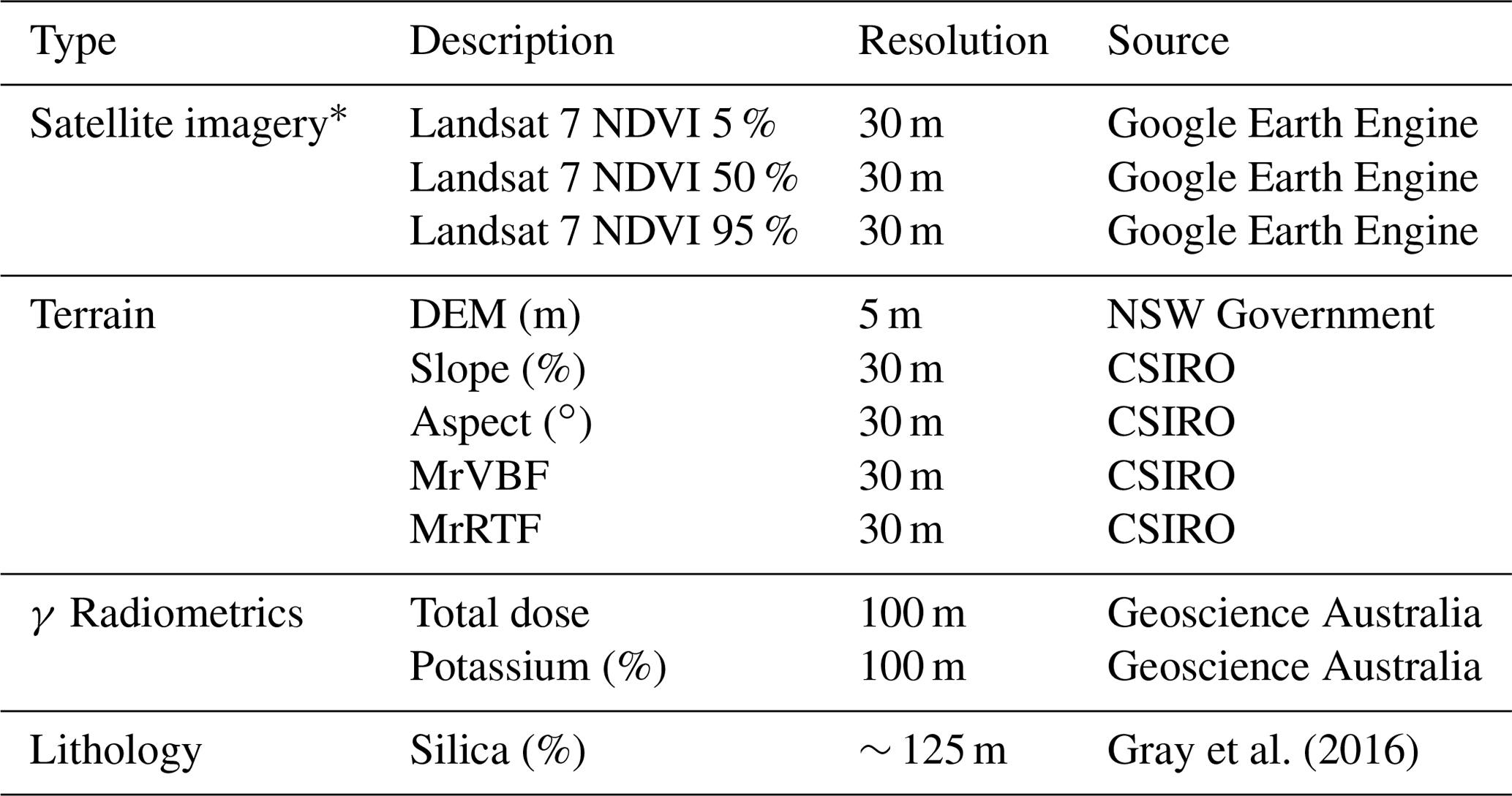
* Landsat 7 NDVI values represent percentiles computed over the 2000–2018 time period.
A 5 m DEM was accessed through the ELVIS (ELeVation Information System) platform (ANZLIC, 2019). This DEM was derived from photogrammetry and generated via airborne imagery; it gives an accurate point estimate of elevation, though it is not hydrologically enforced. Shuttle Radar Topography Mission (SRTM)-derived terrain attributes at 30 m resolution were also accessed through CSIRO's Data Access Portal (CSIRO, 2019). The specific terrain attributes obtained included aspect, multi-resolution ridgetop flatness (MrRTF), MrVBF, and slope. Gridded gamma radiometric data at 100 m spatial resolution derived from an airborne gamma ray spectrometer were obtained through the Geophysical Archive Data Delivery System (GADDS) (Geoscience Australia, 2019). Variation in the concentrations of the radio-elements in this product are indicative of change in soil type or parent material. The individual datasets used included dose rate and potassium concentration data, which were processed with low-pass filtering (Minty et al., 2009). A map of silica index, which is essentially a map of silica content of soil parent material, was also used as a covariate (Gray et al., 2016). The silica index is known to relate to soil texture and other important soil physical properties, such as water holding capacity.
2.6 Modelling and mapping procedure
A regression-kriging approach was utilised to map SI across the study area. All data handling and processing was performed in the R platform for statistical computing (R Core Team, 2019). The dataset was split into a training set (n = 108) and a test set (n = 50) as previously defined. At each of the 108 sampling sites in the training set, the spatial covariates described in Table 1 were extracted using the nearest-neighbour method. A Cubist model was then used to build a relationship between SI and the spatial covariates at each observation point (Kuhn and Quinlan, 2020). A 20 m grid of the study area was created, and the spatial covariates were then extracted using the nearest-neighbour method at each grid point. The developed Cubist model was then used to predict SI on this grid of the study area. The residuals (difference between the observed and predicted SI values) at observation points showed a weak spatial autocorrelation. A Gaussian function fit to the empirical semivariogram had a relatively large nugget of 0.81, sill of 1.11, and range of 1.92 km. A grid of kriged residuals was constructed and added to the mapped output of the Cubist model to obtain the final SI prediction map of the study area. The complexity of the Cubist model was fine-tuned using a leave-one-out cross-validation (LOOCV) approach on the training set. The external validation test set consisting of 50 sites was used to assess the final model. Validation metrics used to assess the prediction performance were Lin's concordance correlation coefficient (LCCC), root-mean-square error (RMSE), bias, and the coefficient of determination (R2).
2.7 Mapping the simulated effect of increased soil organic carbon on slaking index
Relationships between SI and measured soil properties were explored to identify potential contributing factors as a means to inform management practices to reduce excessive slaking. Two classes of soils were evident in the samples, soils with clay content ≥25 % and CEC : clay ratio ≥0.5 which consistently exhibited excessive slaking, and other soils. Class-based regression was used to construct individual predictive models between SI and other measured soil attributes for each class using either multiple linear regression or segmented, non-linear regression for more complex relationships (Baty et al., 2015). The effect of increasing soil OC levels on SI was investigated by simulating increases of 0.5 and 1.0 % OC and applying the relevant class-based regression equation using the laboratory data at each point. These modified SI values were then extrapolated across the study area using the same regression-kriging approach as described above and validated using a LOOCV approach.
3.1 Investigating slaking index variation
3.1.1 Slaking index and soil properties
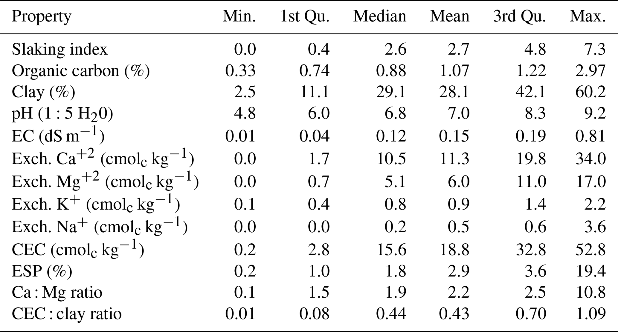
A large range in SI was observed for the samples analysed in this study (Table 3). A minimum SI of 0 was observed for nine samples, meaning that no slaking or swelling occurred and the footprint area of these soil aggregates did not increase. A maximum SI of 7.3 was observed, meaning that the average footprint area for these aggregates is projected to increase in size by 730 %. This indicates an extreme level of aggregate disintegration, although it remains below the maximum theoretical SI of 7.8 suggested by Fajardo et al. (2016). Organic C had an observed range of 0.33 to 2.97 % and a median value of 0.88 %, demonstrating that many of the sampled locations had low levels of OC. Other measured soil properties ranged widely, demonstrating the diversity of soils sampled; for example clay ranged from 2.5 to 60.2 %, and pH ranged from 4.8 to 9.2.
Table 3Summary statistics of slaking index and laboratory-derived soil properties.
Slaking index was positively correlated with clay content (r = 0.84), pH (r = 0.70), electrical conductivity (r = 0.44), CEC (r = 0.87), CEC : clay ratio (r = 0.84), and all exchangeable cations (Table 4). Weak negative correlations were observed for SI with OC (r = −0.31) and Ca : Mg (r = −0.26). These observations support the findings of Fajardo et al. (2016) that SI was positively correlated with pH, clay content, and exchangeable Na+ and Mg+2, and negatively correlated with Ca : Mg. The strongest correlation with SI in this study was observed with exchangeable Mg+2 (r = 0.90). This is in contrast to a recent study that demonstrated exchangeable Mg+2 played a negligible role in flocculation of soil particles and aggregate stability (Zhu et al., 2019). It is believed that the observed correlation in our study is due to the dependence of exchangeable Mg+2 on clay content, CEC, and shrink–swell minerals, such as smectite, rather than a direct causal effect. Clay content was a strong indicator of SI potential. Only one sample with clay content <25 % had an observed SI greater than 1; in contrast only three samples with clay content ≥25 % had an observed SI less than 1. Clay soils are often more susceptible to slaking as they have both a higher concentration of shrink–swell minerals and also a greater concentration of smaller pores that may trap and compress air bubbles (Emerson, 1964). The majority of clay soils had a high CEC : clay ratio, indicating that the dominant phyllosilicate in many of the clay soils studied is smectite. No correlation was observed between SI and ESP in our study. Churchman et al. (1993) reviewed causes of swelling and dispersion in Australian soils and identified that exchangeable Na+ increased swelling, but only for high ESP values. Most of the samples in our study had low ESP values, which explains the lack of correlation with SI values. The low ESP values resulted in minimal dispersion observed in these samples, which was beneficial for this study as the SLAKES application currently cannot distinguish between slaking and dispersion (Fajardo et al., 2016).
Table 4Pearson correlation coefficient (r) between soil properties.
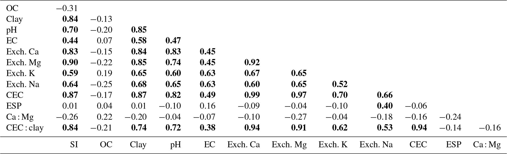
Bold font indicates significance at p<0.05. SI: slaking index; OC: organic carbon; pH: pH (1:5 H2O); EC: electrical conductivity (1:5 H2O); CEC: cation exchange capacity; ESP: exchangeable sodium percentage; Ca : Mg: ratio of exchangeable Ca+2 to Mg+2; CEC : clay: ratio of organic-matter-corrected CEC to clay content.
3.1.2 Slaking index and land use
Land use at sampling sites was categorised into four classes: forest, predominately remnant vegetation cover on sand hills; pasture, encompassing not only improved and unimproved pastures but also stock routes and other areas of perennial grass cover; dryland cropping; and irrigated cropping. Clear differences in SI values were observed under these different land uses, which were accentuated after separating based on clay content (Fig. 2). For samples with clay content ≥25 %, irrigated cropping had the highest SI values, followed by dryland cropping (which showed a large range of SI values) and then pasture. No samples with clay content ≥25 % were observed under forest cover, nor soils with clay content <25 % under irrigated cropping. These findings are supported by the few existing studies investigating SI values of aggregates under cultivated sites compared to paired sites under natural vegetation (Fajardo et al., 2016; Flynn et al., 2020). Decreased aggregate stability of soils under cropping compared to pasture or natural vegetation has also been observed by other indicators of aggregate stability, such as mean weight diameter and water-stable aggregates (Saygın et al., 2012; Ye et al., 2018). The marked differences in soil aggregate stability between land uses may be attributable to the impact of cultivation on the soil – both the direct destruction of aggregates through cultivation and associated increase in soil respiration and loss of OC. The natural disposition of these soils to slake is evident with an average SI of 2.8 observed for soils with ≥25 % clay content under perennial ground cover in the pasture land use. This natural disposition had been significantly exacerbated by cultivation, with an average SI value of 4.8 observed for sites under dryland cropping and 5.0 for sites under irrigation. The difference in mean SI value between irrigated and pasture land uses for clay soils was not found to be significant at the 95 % confidence level (p=0.07), but given the large difference in means this is assumed to be due to the small number of observations for the irrigated clay soils (n=5). The higher level of slaking under irrigation may be due to the fact that irrigated cropping represents a further level of cultivation intensification compared to dryland sites, and sampled irrigated sites also only occurred on soils with clay content >50 %. For the sites with clay content <25 % SI values were predominately <1. Differences between land use were not significant for these low-clay-content soils, although increases in mean values were observed from forest to pasture and then dryland agriculture. A wide range of SI values was observed for samples with ≥25 % clay content, warranting further investigation.
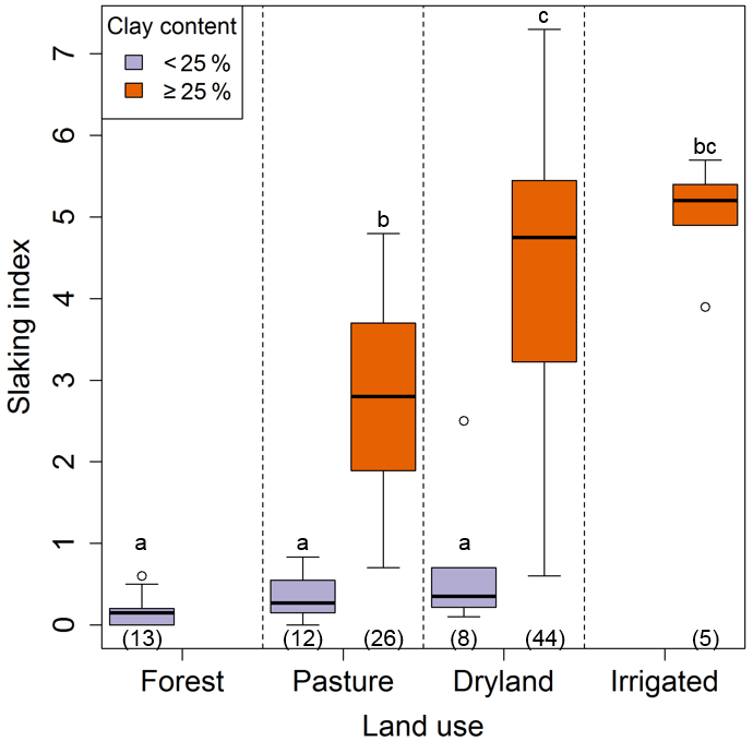
Figure 2Box plots of slaking index grouped by land use (forest, pasture, dryland cropping, or irrigated cropping) and clay content (<25 % or ≥25 %) for the training set. Significant differences between means (p<0.05) of each class calculated using Tukey's honest significant difference test are indicated by a lowercase letter above each plot. The number of observations for each class is indicated in brackets below each plot.
3.1.3 Effect of organic carbon on slaking index
Organic C has been shown to increase soil aggregation and decrease susceptibility to slaking (Six et al., 2000). Chenu et al. (2000) found OC to be a good predictor of soil aggregate stability (R2 = 0.72) when investigating the effects of tillage management on humic loamy soils in south-west France. The diverse range of soils used in this study is assumed to have confounded this relationship as only a weak negative correlation (r = −0.31) between SI and OC was observed, while much stronger correlations were observed for other soil properties, such as clay content or CEC : clay ratio (Table 4). To investigate these correlations further, the relationship between clay content, CEC : clay ratio, and SI was visualised (Fig. 3). CEC : clay ratio was identified as an important parameter as it is an indicator of clay mineral type which affects slaking through its contribution to the shrink–swell characteristics of a soil. A correlation between clay content and CEC : clay ratio was observed (Table 4). This relationship was related to landscape position in the study area, as high-clay-content soils found in floodplain areas also contained a higher proportion of shrink–swell clay minerals, such as smectite. Meanwhile, topsoil samples from the hills and slopes had lower clay content and also a lower CEC : clay ratio, indicating the dominance of low-CEC phyllosilicates, such as kaolinite or illite. As identified previously, samples with clay content <25 % showed minimal slaking. For samples with a clay content ≥25 %, CEC : clay ratio was an important predictor of slaking. For example, soils with a clay content ∼ 40 % showed low-to-moderate slaking for CEC : clay ratio <0.5 and moderate-to-extreme levels of slaking for CEC : clay ratio >0.5 (Fig. 3). Clear threshold values were observed, with extreme slaking values only occurring for soils clay content ≥25 % and CEC : clay ratio >0.5. This observation was used to allocate samples into two classes: samples with clay content ≥25 % and CEC : clay ratio >0.5, and all remaining samples. Relationships between measured soil properties and observed SI values were modelled independently for each class as different critical values were expected to control behaviour of different soil classes (Loveland and Webb, 2003).
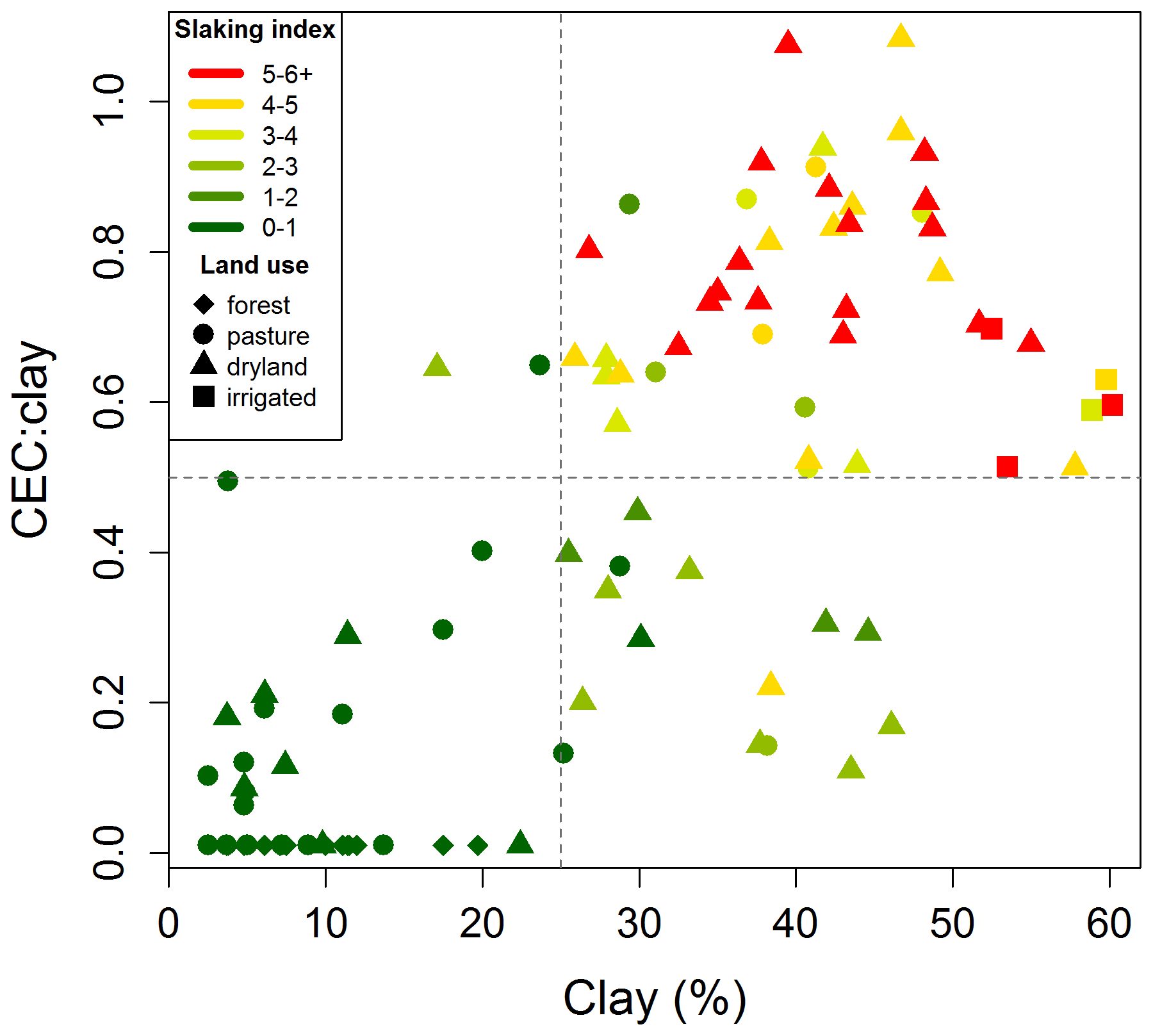
Figure 3Relationship between clay content, CEC : clay ratio, and slaking index (SI). Land use at sample site is indicated as forest, pasture, dryland cropping, or irrigated cropping. Dashed lines indicate clay content of 25 % and CEC : clay ratio of 0.5, above which extreme slaking was observed.
Soil organic carbon was the only significant predictor of SI for soils with clay content ≥25 % and CEC : clay ratio >0.5. The relationship between SI and OC fit a segmented, exponential decay function (Fig. 4). This equation was developed by optimising a four-parameter non-linear regression model to minimise residual sum of squares using the nls function from the nlstools R package (Baty et al., 2015). The model contained a constant value that characterised SI behaviour under low OC levels, a threshold value above which the relationship was characterised by exponential decay, and two parameters that characterised exponential decay behaviour at high OC levels. A threshold value of 1.1 % OC was identified. The average observed SI value for samples below this threshold was 5.01. Extreme SI values were uniquely observed for samples with OC content under this threshold value. As the constant value indicates, no relationship between OC and SI was identified for these samples, nor could a relationship be developed between SI and other measured soil properties. As such the factors responsible for the large range in observed SI values for these soils remain unidentified. To identify causal factors, future research should investigate potential relationships between SI and OC fractions, OC type, microbial activity, or crop species that have been previously identified as influencing aggregate stability (Six et al., 1998; Morel et al., 1991; Blankinship et al., 2016). The 1.1 % threshold value also effectively separated observed differences in OC content between pasture and cropping land use activities. Interestingly, pasture sites with ∼ 1.0 % OC had lower observed SI values than corresponding dryland agriculture sites, indicating that direct effects of cultivation, extended fallow, or monoculture production may influence observed SI values, although the number of samples is too small for statistical analysis. Similar critical OC content values ranging from 1.1 to 2 % have been identified when considering a soil's ability to provide nutrients for crop growth or support microbial diversity (Aune and Lal, 1997; Zvomuya et al., 2008; Yan et al., 2000). For this study the 1.1 % OC value should not be interpreted as a target value for farm managers to achieve, but rather it describes an absolute minimum threshold below which slaking is unpredictable and can result in extreme values. To abate potentially detrimental effects of slaking, farm managers should aim to increase OC levels above this minimum threshold. The exponential decay component of the equation provided a weak fit to the available data (R2 = 0.27). The function suggests that slaking can be reduced, but not completely eliminated, by increasing OC content for the range of OC contents observed in this study. The constant parameter of 2.76 in the exponential decay function suggests a minimum obtainable SI value for these soils; however this model was based on few observations and limited samples of >2 % OC. Future investigation should prioritise identification of sites with higher OC content to better characterise this relationship.
The relationship between SI and OC for the soils that did not meet the criteria of ≥25 % clay content and CEC : clay ratio >0.5 was modelled separately using multiple linear regression. For these soils, SI was explained with the following equation: SI = −0.22 − 0.19 ×OC + 0.09 ×clay (R2=0.77, RMSE = 0.7, p = 0.000). This regression equation indicates that, while OC content still had a significant effect on observed SI values, the magnitude of the effect is lower for these soils. For example, soils with clay content ≥25 % and CEC : clay ratio >0.5 are expected to see a reduction in SI of 1.59 units if OC is increased from 0.7 to 1.7 %; meanwhile if OC is increased from 0.7 to 1.7 % in other soils, a decrease in SI of only 0.19 is expected to occur. These two equations were used to model the effect on SI of simulated 0.5 and 1.0 % increases in OC at the sample sites, which were then mapped across the study area. The results of these analyses are shown in Sect. 3.2.4.
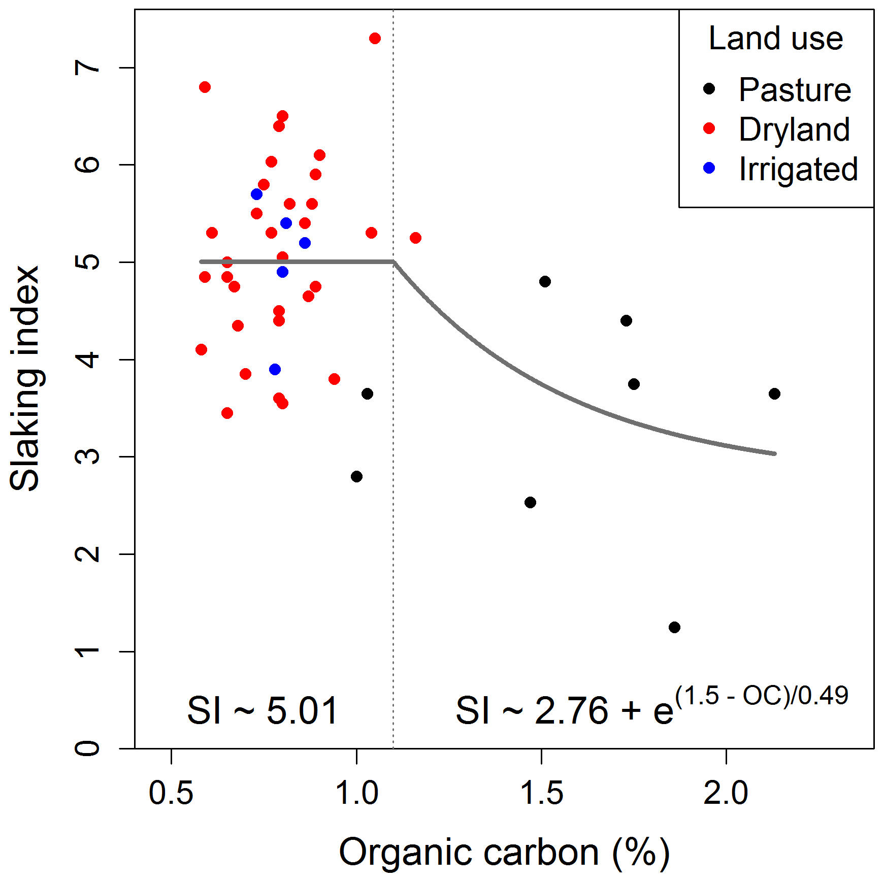
Figure 4Relationship between slaking index (SI) and organic carbon (OC) for soil samples with clay content ≥25 % and CEC : clay ratio >0.5. A segmented, exponential decay function containing a lag phase and threshold value of 1.1 % OC was fit to the observed data points. Land use at each observation point is indicated.
3.2 Mapping results
3.2.1 Importance of predictor variables
Investigation of the use of covariates as conditions and predictors in the Cubist model showed that MrVBF and the NDVI 5th, 50th, and 95th percentiles were the most important predictor variables of SI values. The NDVI data used in this study largely represent variation in vegetation cover and, hence, land use. The 5th percentile of NDVI was used as both a condition and a predictor in the model. The 5th percentile of NDVI represents the lower distribution of vegetation over the 2000–2018 period, with low values indicating cultivated sites (Chen et al., 2018) and variation within cultivated sites representing topsoil variability. Low values of the 5th percentile of NDVI indicate areas of bare earth from cultivation or extended fallow, facilitating the identification of cropping sites. For cropping sites, the 5th-, 50th-, and 95th-percentile values would be vastly different due to the seasonal nature of cropping. This would be similar in the pastures due to seasonal “browning off” of the perennial grass cover. In contrast, the different NDVI percentiles for forest cover would be high and relatively similar due to the more constant biomass throughout different seasons. The importance of NDVI percentiles in the model and known relationships with land use support previous findings that land use has a considerable influence on observed SI values (Fig. 2). The importance of MrVBF may be attributed to the information it contains on landscape position, which is related to clay content and CEC : clay ratio (Gallant and Dowling, 2003). The lowest MrVBF values were found on the sand hills, increasing through a transition zone to the upper floodplain. The highest MrVBF values were found on the lower floodplain, which also corresponded to the highest clay content in the study area. Slope and gamma radiometric potassium data were used as predictors in the model. The important predictors in the model reflect those used by Ye et al. (2018) to map aggregate stability in a small catchment of the Loess Plateau, which the authors found was explained by intrinsic factors (parent material, terrain attributes, and soil type) and extrinsic factors (land use and farming practice). The covariates that were the least important predictors included elevation, MrRTF, and aspect.
3.2.2 Mapping accuracy
The quality of the predictions of SI from the regression-kriging approach was assessed using two validation techniques. The first technique involved using LOOCV on the training dataset (n = 108). This method showed that SI could be predicted to a relatively high degree of accuracy, with an LCCC of 0.85, R2 of 0.75, RMSE of 1.1, and bias of 0.0 (Fig. 5). The second approach involved comparing SI values observed for an independent test set (n = 50) with SI values extracted from the final map product. The second approach demonstrated the robustness of the model, as SI was predicted with similar accuracy to that of the training set, with an LCCC of 0.82, R2 of 0.78, RMSE of 1.1, and bias of 0.6 (Fig. 5). This demonstrates that SI can be accurately spatially predicted when using DSM techniques and ancillary spatial information. The successful prediction of SI can be attributed to availability of ancillary spatial information that explains the main factors controlling slaking, such as the different NDVI percentiles representing land cover and use, and MrVBF representing clay content and the accumulation of water and soil deposition across the landscape. While there are no other published studies to our knowledge that have modelled and mapped SI across a study area, these validation statistics are comparable to other DSM studies that have modelled other aspects of soil stability, such as Annabi et al. (2017), who modelled aggregate stability using three different indices in a study region in Tunisia, with an accuracy of 0.62 to 0.74 R2 when tested with LOOCV.
3.2.3 Spatial variability of slaking index
The map of soil SI across the study area shows considerable variation (Fig. 6). The model was very effective at mapping high-clay-content soils that had a natural tendency to slake and also at identifying tillage practices that exacerbated this effect. It is clear that SI values were higher in arable areas, particularly on the cropped fields at L'lara, as well as the dryland and irrigated cropping areas lower down the floodplain to the south-west of L'lara. The forested areas showed the lowest SI values in the study area. The spatial patterns of the maps are clearly driven by vegetation cover and MrVBF, as indicated by the variables used as conditions and predictors in the Cubist model. The unique features of MrVBF can be seen, as low SI values are found where deposition would be low, whereas high SI values are found where deposition is expected to be high. The NDVI 5th-percentile covariate provides a good indication of whether a field has undergone tillage or been left in a bare fallow but provides no insight into the frequency, timing, or intensity of tillage events. An aspect for further improvement to this approach would be to include a more sensitive method able to characterise the frequency of tillage events or quantify the amount of time left under bare fallow.

Figure 5Plot of observed and predicted slaking index (SI) values from regression kriging for two validation methods: (1) leave-one-out cross-validation (LOOCV) on the training set (n = 108) and (2) external validation on an independent test set (n = 50).
3.2.4 Mapping slaking index after modelled increase in organic carbon
The impact of increasing soil OC levels by 0.5 and 1.0 % on SI values was assessed and mapped across the study area (Fig. 7). When tested with LOOCV, the mapping procedure used for the simulated scenario of a 0.5 % increase in OC was found to have an LCCC of 0.94, R2 of 0.90, RMSE of 0.6, and bias of −0.1, and the simulated scenario of a 1.0 % increase in OC had an LCCC of 0.95, R2 of 0.92, RMSE of 0.4, and bias of 0.0. The validation metrics for the simulated 0.5 and 1.0 % increases in OC were better than those derived from modelling under current conditions. This may be attributed to the simulated map showing a bimodal distribution of SI values, with approximately half of the study area predicted to have SI values of ∼ 0, and the other half predicted to have SI values of ∼ 3 under the scenario of a 1.0 % increase in OC. The reason for this is likely due to SI values returning to their natural or expected values, which are primarily driven by clay content and clay type as opposed to land use and management. Another contributing factor for the improved validation metrics under increased-OC scenarios is that the SI values are based on modelled data from which unexplained error has been removed. Future efforts should account for the error of the underlying regression equations and quantify the uncertainty of the resultant maps by bootstrapping and applying random error based on the prediction variance of the underlying regression equations. The change maps show the difference between the current observed SI values and the simulated SI under increased-OC-content scenarios. These maps reveal a much larger expected decrease in SI values for the scenario of a 1.0 % increase in OC and that the largest decreases in SI values were predicted to occur in dryland and irrigated cropping areas at L'lara and its surrounds. Some of these areas were predicted to have their SI value decreased by up to 3 units. Many of the forested and pasture areas with lower current SI values were predicted to have their SI value largely unchanged even by a 1.0 % increase in OC content. The produced maps highlight areas that are expected to have lower SI when OC levels are increased. This could encourage farmers and land managers to implement management practices that increase soil OC levels in cultivated areas, such as minimal tillage and cover cropping.
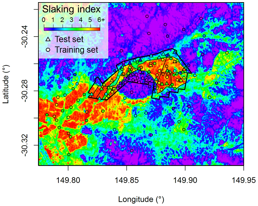
Figure 6Prediction of slaking index (SI) across the study area using regression kriging. The SI values at observation sites for the training set (n = 108) and test set (n = 50) are provided. The external perimeter boundary of L'lara is indicated by the thick black line, and boundaries of cropping paddocks are indicated by thin black lines.
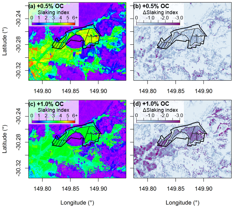
Figure 7Prediction of slaking index across the study area using regression kriging after modelled increases in organic carbon: (a) slaking index after a modelled 0.5 % increase in organic carbon, (b) change in slaking index after a modelled 0.5 % increase in organic carbon, (c) slaking index after a modelled 1.0 % increase in organic carbon, and (d) change in slaking index after a modelled 1.0 % increase in organic carbon. The external perimeter boundary of L'lara is indicated by the thick black line, and boundaries of cropping paddocks are indicated by thin black lines.
Topsoil SI values were obtained through the use of the SLAKES smartphone application to assess aggregate stability in a mixed agricultural landscape. Land use had a clear impact on SI values, with sites under irrigated and dryland cropping showing higher SI values than those under pasture and forested areas. Clay content, CEC : clay ratio, and organic carbon content had a considerable impact on SI values of soil samples. Samples with low OC and high clay content combined with high CEC : clay ratio were the most prone to slaking. An OC threshold of 1.1 % was observed, below which slaking behaviour was not correlated with any of the measured soil properties and the most extreme SI values were observed. A regression-kriging approach utilising a Cubist model and diverse spatial covariates proved to be successful in spatially modelling SI values. The model had high predictive power, with an LCCC of 0.85 and RMSE of 1.1, when using a LOOCV approach on the training dataset (n = 108). The results were also of high quality when assessed using an independent test set (n = 50), with an LCCC of 0.82 and RMSE of 1.1. The decrease in SI expected from a 0.5 and 1.0 % increase in OC content was also simulated and mapped across the study area. The results of these simulations suggested that considerable improvements in SI and soil aggregate stability could be achieved if practices that promote the sequestration of OC were implemented, particularly in cultivated areas. Overall, this study demonstrated that novel approaches to cheaply and rapidly assess the aggregate stability of soil samples could be combined with DSM approaches to create accurate, fine-resolution maps of aggregate stability. These maps have the potential to guide management decisions, whether that be to determine land use and management, such as to minimise cultivation in areas that are prone to slaking, or to increase OC in areas of extreme slaking through the use of minimum tillage or cover cropping.
The data are not publicly available as a large proportion of the training data was acquired on privately owned land and permission has not be obtained to release the data.
EJJ, PF, and ABM designed the experiment and the data analysis method. EJJ, PF, RW, and VP performed the field sampling campaigns. RW and MF collected the slaking index data. EJJ and PF analysed the data. EJ prepared the paper with contribution from all co-authors.
The authors declare that they have no conflict of interest.
The authors would like to thank Blandine Lemercier and Sébastien Salvador-Blanes for their review and valuable suggestions on how to improve the manuscript. The authors would also like to thank Alessandra Calegari, Vita Ayu Kusuma Dewi, Zhiwei (Vera) Wang, Bradley Ginns, Hannah Lowe, and Victoria Pauly for their assistance in gathering and analysing soil samples.
This research was supported by the Grains Research and Development Corporation (grant no. US00087) and the Australian National Landcare Program (grant ID GA25329): DigiFarm – A digitally enabled durable agroecosystem.
This paper was edited by Olivier Evrard and reviewed by Blandine Lemercier and Sebastien Salvador-Blanes.
ABARES: The Australian land use and management classification version 8, Australian Bureau of Agricultural and Resource Economics and Sciences, CC BY 3.0, Canberra, available at: https://www.agriculture.gov.au/abares/aclump/land-use/catchment-scale-land-use-of-australia-update-december-2018 (last access: 11 November 2020), 2018. a
Annabi, M., Raclot, D., Bahri, H., Bailly, J. S., Gomez, C., and Le Bissonnais, Y.: Spatial variability of soil aggregate stability at the scale of an agricultural region in Tunisia, Catena, 153, 157–167, https://doi.org/10.1016/j.catena.2017.02.010, 2017. a, b
ANZLIC: ELVIS – Elevation and Depth – Foundation Spatial Data, available at: https://elevation.fsdf.org.au/, last access: 20 September 2019. a
Aune, J. and Lal, R.: Agricultural productivity in the tropics and critical limits of properties of Oxisols, Ultisols, and Alfisols, Trop. Agr., 74, 96–103, 1997. a
Barzegar, A. R., Oades, J. M., and Rengasamy, P.: Soil structure degradation and mellowing of compacted soils by saline–sodic solutions, Soil Sci. Soc. Am. J., 60, 583–588, 1996. a
Baty, F., Ritz, C., Charles, S., Brutsche, M., Flandrois, J.-P., and Delignette-Muller, M.-L.: A Toolbox for Nonlinear Regression in R: The Package nlstools, J. Stat. Softw., 66, 1–21, https://doi.org/10.18637/jss.v066.i05, 2015. a, b
Blankinship, J. C., Fonte, S. J., Six, J., and Schimel, J. P.: Plant versus microbial controls on soil aggregate stability in a seasonally dry ecosystem, Geoderma, 272, 39–50, 2016. a
Bureau of Meteorology: Monthly climate statistics – Narrabri West Post Office (053030), available at: http://www.bom.gov.au/climate/averages/tables/cw_053030.shtml, last access: 12 February 2020. a
Chen, Y., Lu, D., Moran, E., Batistella, M., Dutra, L. V., Sanches, I. D., da Silva, R. F. B., Huang, J., Luiz, A. J. B., and de Oliveira, M. A. F.: Mapping croplands, cropping patterns, and crop types using MODIS time-series data, Int. J. Appl. Earth Obs., 69, 133–147, 2018. a
Chenu, C., Le Bissonnais, Y., and Arrouays, D.: Organic matter influence on clay wettability and soil aggregate stability, Soil Sci. Soc. Am. J., 64, 1479–1486, 2000. a, b
Churchman, J., Skjemstad, J., and Oades, J.: Influence of clay minerals and organic matter on effects of sodicity on soils, Aust. J. Soil Res., 31, 779–700, https://doi.org/10.1071/SR9930779, 1993. a
Collis-George, N. and Lal, R.: Infiltration and structural changes as influenced by initial moisture content, Aust. J. Soil Res., 9, 107–116, 1971. a
CSIRO: Data Access Portal, available at: https://data.csiro.au/collections/, last access: 20 September 2019. a
Emerson, W.: The slaking of soil crumbs as influenced by clay mineral composition, Aust. J. Soil Res., 2, 211–217, https://doi.org/10.1071/SR9640211, 1964. a, b, c
Emerson, W.: A classification of soil aggregates based on their coherence in water, Aust. J. Soil Res., 5, 47–57, https://doi.org/10.1071/SR9670047, 1967. a
Emerson, W.: Structural decline of soils, assessment and prevention, Aust. J. Soil Res., 29, 905–921, https://doi.org/102.100.100/253063, 1991. a
Fajardo, M. and McBratney, A.: Slakes: A soil aggregate stability smart-phone app [Mobile application software], version 2.1, available at: https://play.google.com/store/apps/details?id=slaker.sydneyuni.au.com.slaker&hl=en_AU, last access: 19 November 2019. a, b
Fajardo, M., McBratney, A. B., Field, D. J., and Minasny, B.: Soil slaking assessment using image recognition, Soil Till. Res., 163, 119–129, https://doi.org/10.1016/j.still.2016.05.018, 2016. a, b, c, d, e, f, g
Field, D. J., McKenzie, D. C., and Koppi, A. J.: Development of an improved Vertisol stability test for SOILpak, Soil Res., 35, 843–852, https://doi.org/10.1071/S96118, 1997. a
Filippi, P., Jones, E. J., Ginns, B. J., Whelan, B. M., Roth, G. W., and Bishop, T. F.: Mapping the Depth-to-Soil pH Constraint, and the Relationship with Cotton and Grain Yield at the Within-Field Scale, Agronomy, 9, 251, https://doi.org/10.3390/agronomy9050251, 2019. a
Filippi, P., Jones, E. J., and Bishop, T. F.: Catchment-scale 3D mapping of depth to soil sodicity constraints through combining public and on-farm soil databases – A potential tool for on-farm management, Geoderma, 374, 114396, https://doi.org/10.1016/j.geoderma.2020.114396, 2020. a
Flynn, K. D., Bagnall, D. K., and Morgan, C. L.: Evaluation of SLAKES, a smartphone application for quantifying aggregate stability, in high-clay soils, Soil Sci. Soc. Am. J., 84, 345–353, https://doi.org/10.1002/saj2.20012, 2020. a, b
Gallant, J. C. and Dowling, T. I.: A multiresolution index of valley bottom flatness for mapping depositional areas, Water Res. Res., 39, 1347, https://doi.org/10.1029/2002WR001426, 2003. a
Gee, G. and Bauder, J.: Particle size analysis, in: Methods of soil analysis. Part 1: Physical and mineralogical methods, edited by: Klute, A., Soil Science Society of America and American Society of Agronomy, Madison, WI, USA, 383–411, 1986. a
Geoscience Australia: Geophysical Archive Data Delivery System, available at: https://www.ga.gov.au/gadds/, last access: 20 September 2019. a
Gorelick, N., Hancher, M., Dixon, M., Ilyushchenko, S., Thau, D., and Moore, R.: Google Earth Engine: Planetary-scale geospatial analysis for everyone, Remote Sens. Environ., 202, 18–27, https://doi.org/10.1016/j.rse.2017.06.031, 2017. a
Grant, C. and Blackmore, A.: Self mulching behavior in clay soils-Its definition and measurement, Soil Res., 29, 155–173, 1991. a
Gray, J. M., Bishop, T. F., and Wilford, J. R.: Lithology and soil relationships for soil modelling and mapping, Catena, 147, 429–440, 2016. a, b
IUSS Working Group WRB: World Reference Base for Soil Resources 2014, International Soil Classification System for Naming Soils and Creating Legends for Soil Maps., World Soil Resources Reports No. 106, FAO, Rome, 2014. a
Kuhn, M. and Quinlan, R.: Cubist: Rule- And Instance-Based Regression Modeling, r package version 0.2.3, available at: https://CRAN.R-project.org/package=Cubist, last access: 3 February 2020. a
Loveday, J. and Pyle, J.: The Emerson dispersion test and its relationship to hydraulic conductivity, Tech. rep., CSIRO, Australia Division of Soils, 1973. a
Loveland, P. and Webb, J.: Is there a critical level of organic matter in the agricultural soils of temperate regions: a review, Soil Till. Res., 70, 1–18, 2003. a
Minty, B., Franklin, R., Milligan, P., Richardson, M., and Wilford, J.: The radiometric map of Australia, Explor. Geophys., 40, 325–333, 2009. a
Morel, J. L., Habib, L., Plantureux, S., and Guckert, A.: Influence of maize root mucilage on soil aggregate stability, Plant Soil, 136, 111–119, 1991. a
Mullins, C. E., MacLeod, D. A., Northcote, K. H., Tisdall, J. M., and Young, I. M.: Hardsetting Soils: Behavior, Occurrence, and Management, in: Advances in Soil Science: Soil Degradation Volume 11, edited by Lal, R. and Stewart, B. A., Springer New York, New York, NY, USA, https://doi.org/10.1007/978-1-4612-3322-0_2, 37–108, 1990. a, b, c
Oades, J. and Waters, A.: Aggregate hierarchy in soils, Austr. J. Soil Res., 29, 815–828, https://doi.org/10.1071/SR9910815, 1991. a
Odeh, I. O. and Onus, A.: Spatial analysis of soil salinity and soil structural stability in a semiarid region of New South Wales, Australia, Environ. Manage., 42, 265, https://doi.org/10.1007/s00267-008-9100-z, 2008. a
Peel, M. C., Finlayson, B. L., and McMahon, T. A.: Updated world map of the Köppen-Geiger climate classification, Hydrol. Earth Syst. Sci., 11, 1633–1644, https://doi.org/10.5194/hess-11-1633-2007, 2007. a
R Core Team: R: A Language and Environment for Statistical Computing, R Foundation for Statistical Computing, Vienna, Austria, available at: https://www.R-project.org/, last access: 1 September 2019. a
Rayment, G. E. and Lyons, D. J.: Soil chemical methods: Australasia, Vol. 3, CSIRO publishing, Collingwood, Victoria, Australia, 2011. a
Rengasamy, P., Greene, R., and Ford, G.: The role of clay fraction in the particle arrangement and stability of soil aggregates – A review, Clay Res., 3, 53–67, 1984. a
Saygın, S. D., Cornelis, W. M., Erpul, G., and Gabriels, D.: Comparison of different aggregate stability approaches for loamy sand soils, Appl. Soil Ecol., 54, 1–6, 2012. a
Schindelbeck, R., Moebius-Clune, B., Moebius-Clune, D., Kurtz, K., and van Es, H.: Cornell University Comprehensive Assessment of Soil Health Laboratory Standard Operating Procedures, 20–22, 2016. a, b
Six, J., Elliott, E., Paustian, K., and Doran, J. W.: Aggregation and Soil Organic Matter Accumulation in Cultivated and Native Grassland Soils, Soil Sci. Soc. Am. J., 62, 1367–1377, https://doi.org/10.2136/sssaj1998.03615995006200050032x, 1998. a
Six, J., Paustian, K., Elliott, E. T., and Combrink, C.: Soil structure and organic matter I. Distribution of aggregate-size classes and aggregate-associated carbon, Soil Sci. Soc. Am. J., 64, 681–689, 2000. a
Walkley, A. and Black, I. A.: An examination of the Degtjareff method for determining soil organic matter, and a proposed modification of the chromic acid titration method, Soil Sci., 37, 29–38, 1934. a
Yan, F., McBratney, A., and Copeland, L.: Functional substrate biodiversity of cultivated and uncultivated A horizons of vertisols in NW New South Wales, Geoderma, 96, 321–343, 2000. a
Ye, L., Tan, W., Fang, L., Ji, L., and Deng, H.: Spatial analysis of soil aggregate stability in a small catchment of the Loess Plateau, China: I. Spatial variability, Soil Till. Res., 179, 71–81, https://doi.org/10.1016/j.still.2018.01.012, 2018. a, b
Yoder, R. E.: A direct method of aggregate analysis of soils and a study of the physical nature of erosion losses, Soil Sci. Soc. Am. J., 28, 337–351, https://doi.org/10.2134/agronj1936.00021962002800050001x, 1936. a, b
Zhu, Y., Ali, A., Dang, A., Wandel, A. P., and Bennett, J. M.: Re-examining the flocculating power of sodium, potassium, magnesium and calcium for a broad range of soils, Geoderma, 352, 422–428, https://doi.org/10.1016/j.geoderma.2019.05.041, 2019. a
Zvomuya, F., Janzen, H. H., Larney, F. J., and Olson, B. M.: A Long-Term Field Bioassay of Soil Quality Indicators in a Semiarid Environment, Soil Sci. Soc. Am. J., 72, 683–692, https://doi.org/10.2136/sssaj2007.0180, 2008. a