the Creative Commons Attribution 4.0 License.
the Creative Commons Attribution 4.0 License.
 | 17 Nov 2020
The influence of training sample size on the accuracy of deep learning models for the prediction of soil properties with near-infrared spectroscopy data
Budiman Minasny
Wanderson de Sousa Mendes
José Alexandre Melo Demattê
The number of samples used in the calibration data set affects the quality of the generated predictive models using visible, near and shortwave infrared (VIS–NIR–SWIR) spectroscopy for soil attributes. Recently, the convolutional neural network (CNN) has been regarded as a highly accurate model for predicting soil properties on a large database. However, it has not yet been ascertained how large the sample size should be for CNN model to be effective. This paper investigates the effect of the training sample size on the accuracy of deep learning and machine learning models. It aims at providing an estimate of how many calibration samples are needed to improve the model performance of soil properties predictions with CNN as compared to conventional machine learning models. In addition, this paper also looks at a way to interpret the CNN models, which are commonly labelled as a black box. It is hypothesised that the performance of machine learning models will increase with an increasing number of training samples, but it will plateau when it reaches a certain number, while the performance of CNN will keep improving. The performances of two machine learning models (partial least squares regression – PLSR; Cubist) are compared against the CNN model. A VIS–NIR–SWIR spectra library from Brazil, containing 4251 unique sites with averages of two to three samples per depth (a total of 12 044 samples), was divided into calibration (3188 sites) and validation (1063 sites) sets. A subset of the calibration data set was then created to represent a smaller calibration data set ranging from 125, 300, 500, 1000, 1500, 2000, 2500 and 2700 unique sites, which is equivalent to a sample size of approximately 350, 840, 1400, 2800, 4200, 5600, 7000 and 7650. All three models (PLSR, Cubist and CNN) were generated for each sample size of the unique sites for the prediction of five different soil properties, i.e. cation exchange capacity, organic carbon, sand, silt and clay content. These calibration subset sampling processes and modelling were repeated 10 times to provide a better representation of the model performances. Learning curves showed that the accuracy increased with an increasing number of training samples. At a lower number of samples (< 1000), PLSR and Cubist performed better than CNN. The performance of CNN outweighed the PLSR and Cubist model at a sample size of 1500 and 1800, respectively. It can be recommended that deep learning is most efficient for spectra modelling for sample sizes above 2000. The accuracy of the PLSR and Cubist model seems to reach a plateau above sample sizes of 4200 and 5000, respectively, while the accuracy of CNN has not plateaued. A sensitivity analysis of the CNN model demonstrated its ability to determine important wavelengths region that affected the predictions of various soil attributes.
- Article
(2214 KB) - Full-text XML
- BibTeX
- EndNote


There has been an increasing demand for a rapid and cost-effective method as an alternative to conventional laboratory soil analysis. Visible, near and shortwave infrared (VIS–NIR–SWIR) spectroscopy have been proposed to be used as an alternative tool for soil analysis for the last few decades (Bendor and Banin, 1995; Shepherd and Walsh, 2002; Stenberg et al., 2010). This method enables the simultaneous prediction of various properties and has non-destructive characteristics.
Various machine learning models, such as partial least squares regression (PLSR), Cubist, random forest and support vector machines have been utilised to model spectroscopy data. However, the performances of these regression models are dependent on the spectral preprocessing methods (Rinnan et al., 2009) and the size and representativeness of the calibration samples (Kuang and Mouazen, 2012; Ng et al., 2018). Different combinations of the spectral preprocessing methods will result in various model performances. Furthermore, the spectral preprocessing techniques developed for a particular data set might not work for a different data set. Better generalisation can be made by training the model in a larger data set. However, several studies demonstrated that the performance of the machine learning model did not increase significantly, or it even plateaued, as the calibration sample size increased (Figueroa et al., 2012; Ramirez-Lopez et al., 2014; Ng et al., 2018).
Advances in artificial intelligence, such as deep learning, enable the possibility of extracting features from data without hand-engineered features (LeCun et al., 2015), such as preprocessing. Various deep learning convolutional neural network (CNN) models (i.e. AlexNet, VGGnet, GoogLeNet and ResNet) had been developed and trained on large volumes of data, which included over 10 million image data (Krizhevsky et al., 2012; Simonyan and Zisserman, 2014; Szegedy et al., 2015; He et al., 2016). CNN has recently been applied in soil science (Padarian et al., 2019; Tsakiridis et al., 2020). Although CNN often deals with images as input data, it has recently been successfully applied to vibrational and reflectance spectroscopy (Acquarelli et al., 2017; Cui and Fearn, 2018; Liu et al., 2018; Ng et al., 2019; Padarian et al., 2019; Tsakiridis et al., 2020; Zhang et al., 2020). Acquarelli et al. (2017) found that the CNN-based model outperformed other models (partial least square, least discriminant analysis, logistic regression and k nearest neighbour) for the classification of various vibrational spectroscopy data. CNN also has recently been successfully utilised for regression modelling using reflectance spectroscopy data (Cui and Fearn, 2018; Liu et al., 2018; Ng et al., 2019; Padarian et al., 2019). Cui and Fearn (2018) compared the performance of CNN and PLSR to predict the protein and ash content of wheat kernels and wheat flour from the NIR–SWIR spectra with calibration sample size ranging from 415 to 6987. Liu et al. (2018) developed a 1D CNN model using VIS–NIR–SWIR spectra to predict clay content with a calibration sample size of 16 000. Other studies have shown that the CNN model has the capability to outperform the PLSR and Cubist model for the prediction of various soil properties using VIS–NIR–SWIR (Ng et al., 2019; Padarian et al., 2019), mid-infrared (MIR) and combined VIS–NIR–SWIR with MIR spectra (Ng et al., 2019) with a calibration sample size greater than 10 000.
These days, deep learning, such as CNN, that was developed to handle a large amount of data (millions of images) and soil spectra is not that large yet. For example, a recent study used deep learning on 135 soil samples (Chen et al., 2018). The advantage of using CNN on such a small number of samples is uncertain. A recent review on spectroscopy showed that there were several studies in which deep learning was used with a small calibration sample size (Yang et al., 2019). The review indicated that an increase in calibration sample size should further improve the calibration performance. However, there was no guideline as to how much improvement can be expected and what the minimum number of samples was for it to be effective.
A strategy to select an adequate calibration set in terms of representativeness and size is vital for obtaining a model with good generalisation ability. Although various sampling algorithms (e.g. Kennard–Stone, conditioned Latin Hypercube sampling and k means clustering) to select representative samples have been explored (Ramirez-Lopez et al., 2014; Ng et al., 2018), the question of how many samples are needed for the CNN model to perform better than machine learning models for spectroscopy data has yet to be determined. It is commonly depicted and hypothesised in a learning curve that, as more data are available, CNN will outperform traditional machine learning models (Mahapatra, 2018; see Fig. 1). Machine learning models tend to reach a plateau or show marginal improvement with an increasing amount of data, as the model has limited complexity to deal with an increasing amount of data (Zhu et al., 2016).
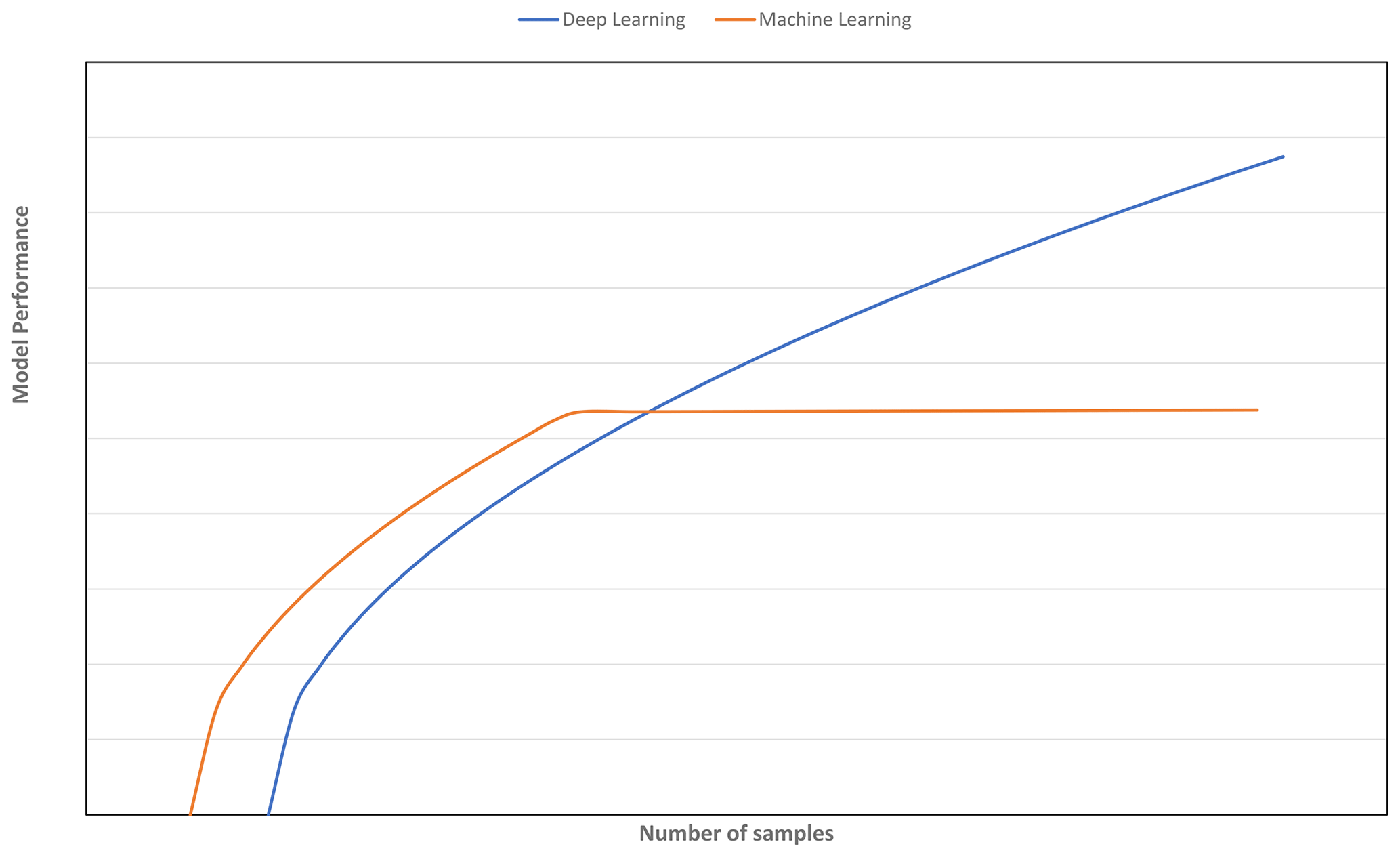
Figure 1Model performance of deep learning vs. other machine learning algorithms as a function of number of samples.
Thus, the purpose of this study is to assess the amount of calibration data needed for the CNN model to outperform machine learning models. PLSR and Cubist are chosen as the representatives of the machine learning models which have been found to perform well in soil spectra (e.g. Dangal et al., 2019). In addition, to be able to predict soil properties accurately, we need to understand and interpret how a CNN model can predict soil properties from spectra. This paper presents the following specific contributions:
-
testing the idea that common machine learning models will reach a plateau in accuracy with an increasing number of calibration samples,
-
establishing the number of calibration samples required for deep learning to be effective for VIS–NIR–SWIR spectra,
-
establishing how much improvement in accuracy is achieved when the number of calibration samples for deep learning and machine learning models is increased, and
-
demonstrating how to interpret a deep learning model using a sensitivity analysis.
2.1 Data set and chemical analysis
This data set comprises 12 044 soil samples from 4251 unique sites. The soil samples, collected from several regions in Brazil, i.e. the states of São Paulo, Minas Gerais, Goiás and Mato Grosso do Sul. This data set is part of the Brazilian Soil Spectral Library and has been extracted from Terra et al. (2018) and Bellinaso et al. (2010). The soils were derived mostly from basalt (volcanic rock) and sedimentary rocks (sandstone). Each site has up to seven measurements from the surface up to 1 m depth.
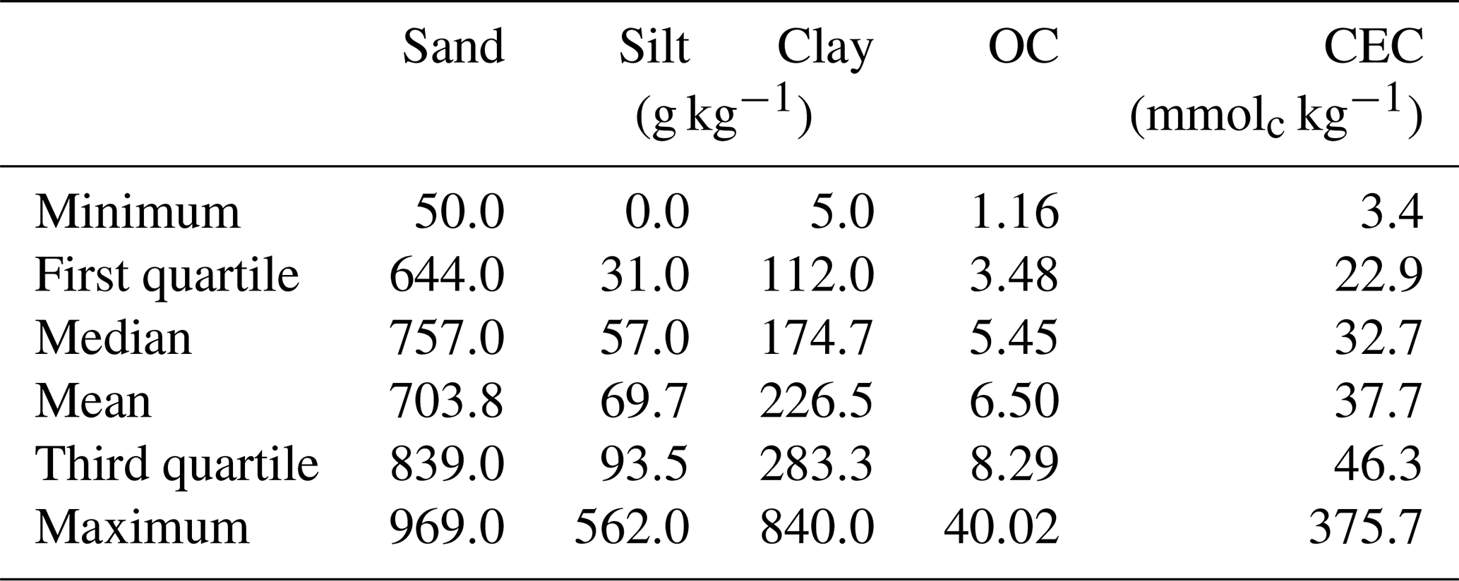
The measured properties include soil texture (sand, silt and clay), organic carbon (OC) and cation exchange capacity (CEC). The soil particle size was quantified by the pipette method, as described in Donagema et al. (2011). The method consists of using a 0.1 M NaOH solution as a dispersing agent under high-speed mechanical stirring for 10 min. Then, the sand fraction was separated by sieving, and the clay fraction was measured by sedimentation. The silt was quantified based on the pre- and post-difference. Organic carbon (OC) was determined by the Walkley–Black method (Walkley and Black, 1934), in which OC was oxidised, using K2Cr2O7 in a wet environment, and then measured by titration with 0.1 M ammonium iron sulfate. As described in Donagema et al. (2011), a 1 M KCl solution was used to extract aluminium, exchangeable calcium and magnesium. The atomic absorption spectrophotometry was used to quantify Ca and Mg concentrations. Aluminium concentration was determined by titrating with 0.025 M NaOH. Potassium was extracted using a Mehlich 1 (0.05 M HCl with 0.0125 M H2SO4) solution, and the K concentration was measured using the flame photometry. Afterwards, CEC was determined as the sum of exchangeable cations. The descriptive statistics of the soil properties measured are included in Table 1.
Table 1Descriptive statistics of the soil properties measurements.
2.2 Spectra measurements
The VIS–NIR–SWIR spectra of the soil samples were obtained with a FieldSpec3 spectroradiometer (Analytical Spectral Devices, Boulder, Colorado), with a spectra range of visible to shortwave infrared (350–2500 nm) and a spectra resolution of 1 nm from 350 to 700 nm, of 3 nm from 700 to 1400 nm and of 10 nm from 1400 to 2500 nm. The sensor scanned an area of approximately 2 cm2, and a light source was provided by two external 50 W halogen lamps. These lamps were positioned at a distance of 35 cm from the sample (non-collimated rays and a zenith angle of 30∘), with an angle of 90∘ between them. A Spectralon (Labsphere, Inc., North Sutton, NH) standard white plate was scanned every 20 min during calibration. The samples were oven-dried at 45 ∘C for 48 h before being ground and sieved ≤2 mm. The sample was distributed homogeneously in Petri dishes for spectra measurement. Three replicates (involving a 180∘ turn of the Petri dish) were obtained for each sample. Each spectrum was averaged from 100 readings over 10 s.
2.3 Training and validation
To better represent the soil distribution, we split and subset the data based on sites. The data set was first randomly split into 75 % calibration (3188 sites) and 25 % validation (1063 sites) based on the unique sites.
From the calibration data set, smaller sample sizes ranging between 125, 300, 500, 1000, 1500, 2000, 2500 and 2700 unique sites were created, which is equivalent to a sample size of approximately 350, 840, 1400, 2800, 4200, 5600, 7000 and 7650. Better representations of model performances were provided by 10 replicates of these sizes. Each sampling for the same number of sites could generate a slightly different number of samples, since the number of measurements varied from one site to another. However, the model performance was evaluated on the common validation data set using a total of 1063 sites (sample size N=3017). Thus, we created a learning curve of the accuracy of the models of the validation data set as a function of the number of calibration samples.
2.4 Chemometrics model
Prior to the development of machine learning models (PLSR and Cubist), the spectra were subjected to some preprocessing methods, namely the (i) conversion to absorbance followed by (ii) a Savitzky–Golay smoothing filter, with a window size of 11 and second-order polynomial (Savitzky and Golay, 1964), (iii) spectra trimming to discard region that has a low signal-to-noise ratio (<500 nm and between 2450–2500 nm) and (iv) a standard normal variate (SNV) transformation (Barnes et al., 1989). For the CNN model, the spectra were only normalised with SNV before being fed into the model. Our previous research (Ng et al., 2019) found that CNN has its own filtering algorithm that makes preprocessing unnecessary. This filtering approach will be discussed in the results section.
2.5 PLSR model
PLSR is one of the standard and most commonly used models with spectroscopy data. It is a linear chemometric regression model that projects spectra into latent variables that explain the variances within the spectra and the response variables (Wold et al., 1983). The optimal number of latent variables used in the PLSR regression that resulted in the smallest root mean square error (RMSE) using the cross-validation approach was used to create the models. PLSR was implemented in the R statistical software (R Core Team, 2019) using the “pls” package (Mevik et al., 2018).
2.6 Cubist model
Cubist is a rule-based data mining model, which is an extension of the M5 model tree by Quinlan (1993). Cubist has been used successfully in soil spectroscopy studies and, in many cases, has been found to perform better than PLSR and other machine learning models (Dangal et al., 2019). Cubist creates one or more rules so that, if the rules are met, a certain linear model can be utilised to predict the target task. The model was evaluated using the “Cubist” package (Kuhn and Quinlan, 2018) in R.
2.7 CNN model
The CNN model is composed of three types of layers, namely the convolutional, pooling and fully connected layer. The convolutional layer extracts features from the inputs, the pooling layer reduces the dimensionality of the input feature and the fully connected layer connects the outputs from previous layers to the desired target outputs. The CNN model utilised in this study was derived from our previous study (Ng et al., 2019), in which the spectra were fed into the model as 1D data. The architecture of the CNN model is included in Table 2 and Fig. 2. Some of the layers within the network are shared to enable simultaneous output predictions.
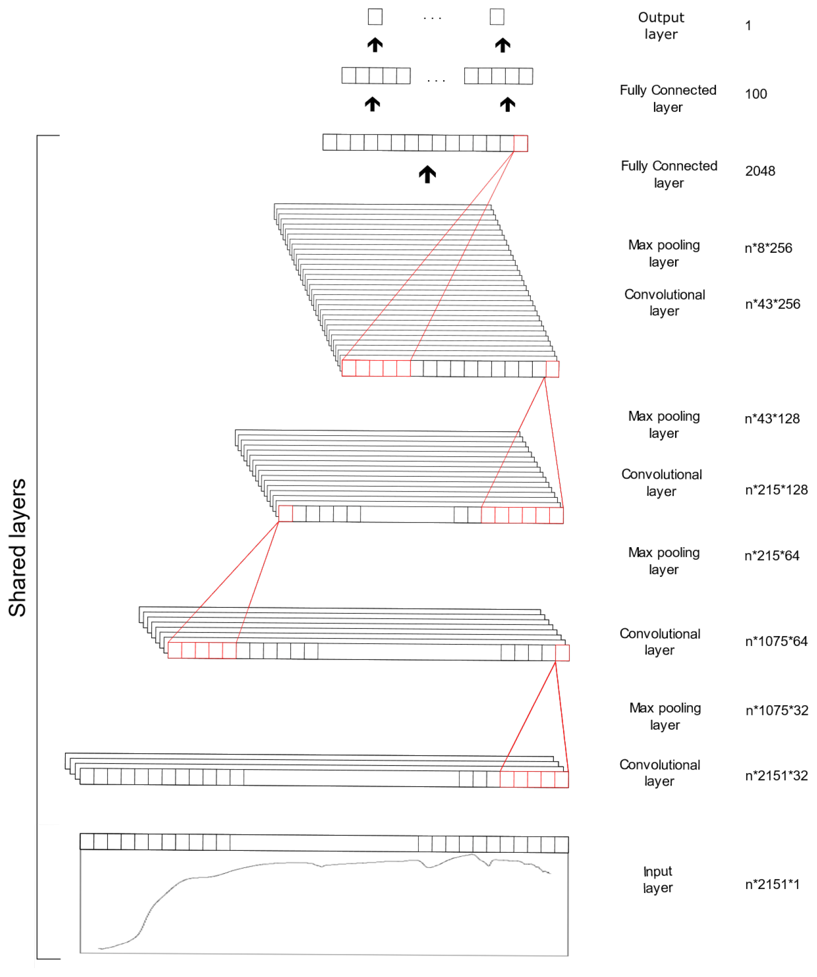
Table 2Architecture of the convolutional neural network model.

ReLUs – rectified linear units.
The CNN model was trained with an initial learning rate of 0.001 and an Adam optimiser (Kingma and Ba, 2014). The network was trained using a batch size of 50 and a maximum epoch of 200. For model optimisation purposes, the calibration data are further divided into a 75 % training and a 25 % testing set. Drop out, early stopping and reduced learning rates are used as a regularisation technique to prevent network overfitting. For further details of the CNN model, the reader is referred to Ng et al. (2019). The CNN model was implemented in Python (version 3.5.1; Python Software Foundation, 2017) using the Keras library (version 2.1.2; Chollet, 2015) and TensorFlow (version 1.4.1; Abadi et al., 2015) back end.
All the model performances were compared in terms of the coefficient of determination (R2) and the root mean square error (RMSE), bias and ratio of performance to interquartile distance (RPIQ) values based on the validation data set. Generally, larger values of R2 and RPIQ and smaller bias and RMSE indicate better model performance.
2.8 Sensitivity analysis: evaluating important wavelengths
To uncover how CNN predicts different soil properties, a sensitivity analysis was conducted to assess the importance of each wavelength in contributing to predictions. Evaluating the sensitivity of the model can be done in several ways; for example, Cui and Fearn (2018) calculated the sensitivity of a CNN model for NIR by taking a numerical partial derivative of the output with respect to each wavelength. For wavelength i, the sensitivity S was calculated as follows:
where X is the reflectance spectra, f(X)i is the CNN prediction using the spectra, and ε is a small number. The idea is that if wavelength i has an important contribution to the prediction, then a small perturbation to the reflectance value will create a large change in the prediction.
In our previous study (Ng et al., 2019), we calculated the sensitivity as a function of the variance of the model for each window of spectra. Here, we calculated the sensitivity based on the variance principle as an alternative approach, as follows:
where Var is the variation calculation, is the prediction of spectra due to the variation in wavelength i with other wavelengths held constant at their mean values, and is the prediction value using the mean values of the spectra and Y is the observed values of the target variable. In essence, we calculated how the model varied in comparison to the observations as a function of wavelength.
The current sensitivity analysis (Eq. 2) considered the actual variance of the data for a better approximation of the wavelength's sensitivity. To calculate the variance sensitivity, two new data frames were created. The first data frame contained data which was the average of all the validation spectra (), and the second contained modified average spectra () in which some of the average measurements were replaced with the actual spectra reflectance at a wavelength width of 5 nm.
The illustrations of the process of deriving new data frames are included in Fig. 3. Both data frames were then fed into the pretrained CNN model (f( )). The variance between the average and modified average spectra were then compared to the actual variance of the target properties as a measure of the model sensitivity (Eq. 2).
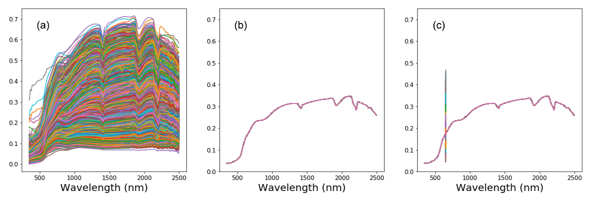
Figure 3Illustration of the sensitivity analysis process, with (a) the validation spectra, (b) the overall average of the validation spectra and (c) the modified average of the validation spectra.
3.1 VIS–NIR–SWIR spectra characteristics
Large variability within the soil properties and texture could potentially influence the soil spectra characteristics (shown in Fig. 4). In general, there was an increase in reflectance between 400 and 1000 nm, with several prominent absorption features at 1400, 1900 and 2200 nm. There are absorption features in the VIS–NIR (400–1000 nm), which are related to iron oxides, such as haematite (Fe2O3) and goethite (FeOOH; Clark, 1999). Absorption near 1400 nm is associated with the first overtone of an O–H stretch vibration of water or metal–O–H vibration, while absorption is 1900 nm is combination vibrations of water related to H–O–H bend and O–H stretch (Viscarra Rossel et al., 2009). Absorption in the 2100–2400 nm region is related to the combination vibrations of minerals. Generally, spectra that have a higher clay content would show smaller reflectance (greater absorption) values in comparison to those with lower clay content. The representative samples of the VIS–NIR–SWIR spectra before and after preprocessing were included in Fig. 4.
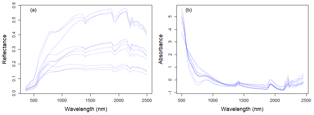
Figure 4Visible, near and shortwave infrared (VIS–NIR–SWIR) spectra of 10 soil samples without spectral preprocessing (a) and with spectral preprocessing (b).
3.2 Visualisation of the spectra within CNN model
An attempt to take a look at what the CNN model actually learns was conducted. As the raw reflectance spectrum was fed into the CNN model, it passed through a convolutional layer which extracted information from the spectra. Filters from the first two convolutional layers were included in Fig. 5. Though only raw spectra were fed into the CNN model, we could see that the spectra underwent some spectral preprocessing within each filter of the layers. Some of the filters shown in the first convolution layer looked like the input spectra pattern (filter nos. 3, 4 and 10), and some of them mimicked the transformation pattern, namely absorbance (filter nos. 1, 5, 6, 7, 9, 13 and 16) and derivatives (filter nos. 2, 8, 11, 12, 14 and 15). The spectrum became smoother when they passed through the second convolutional layer, where some filters only accentuated certain peaks (Fig. 5).
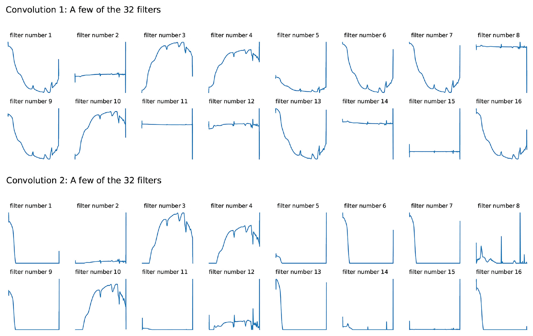
Figure 5Visualisation of the filters in the first two convolutional layers within the 1D convolutional neural network (CNN) model of the visible, near and shortwave infrared (VIS–NIR–SWIR) spectra.
3.3 Prediction of soil properties and model comparison
The model performances for the validation data set using the full calibration data (nsite=3188, N=9027) for various soil properties and chemometrics model were presented in Table 3. The CNN model outperformed both Cubist and PLSR models (in terms of higher R2 and RPIQ and lower RMSE).
Table 3Results of model validation for the prediction of various soil attributes using the full calibration data set.
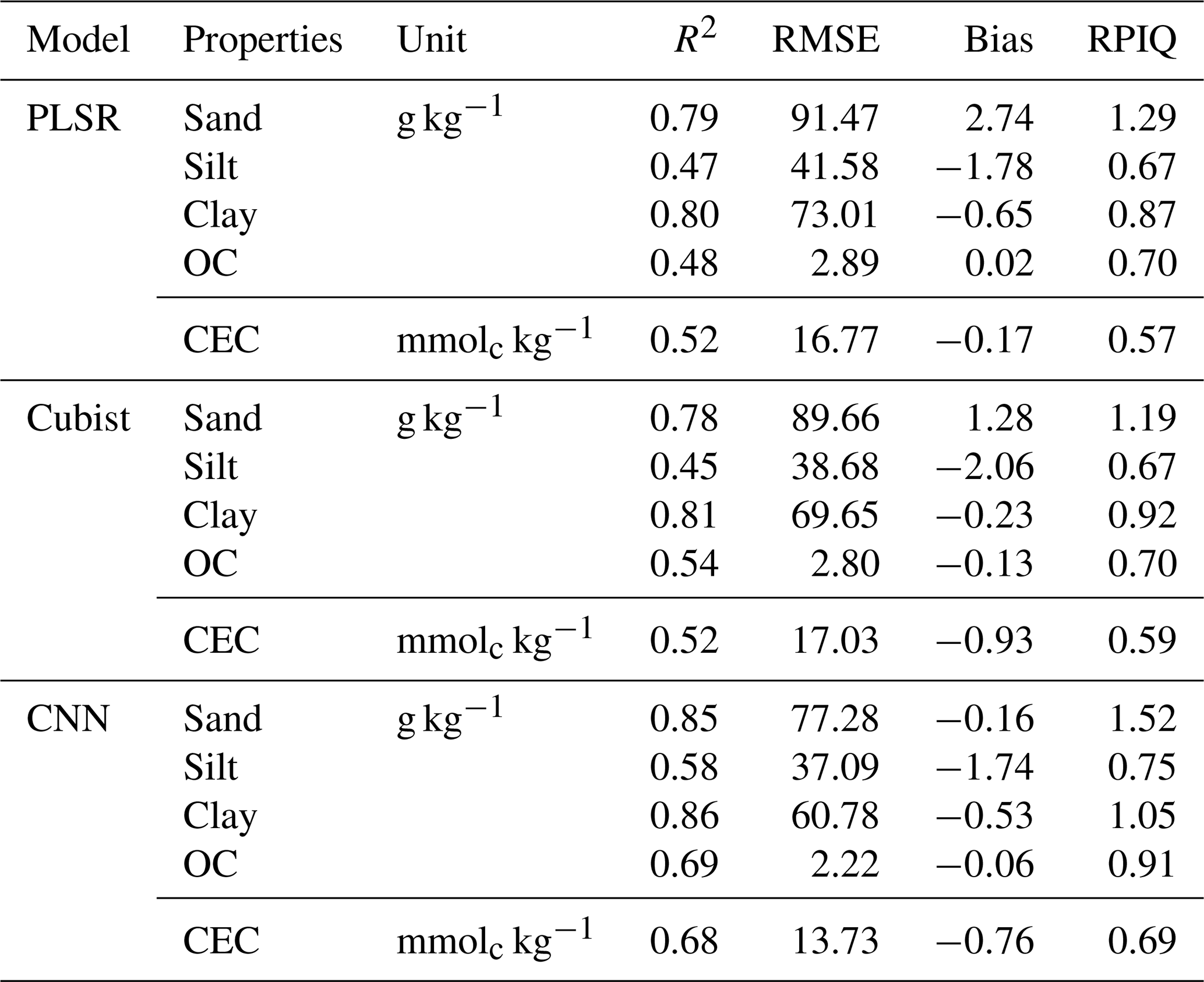
OC – organic carbon; CEC – cation exchange capacity.
The performance was achieved using the CNN model with the prediction of sand (R2=0.85; RPIQ = 1.52), silt (R2=0.58; RPIQ = 0.75), clay (R2=0.86; RPIQ = 1.05), OC (R2=0.69; RPIQ = 0.91) and CEC (R2=0.68; RPIQ = 0.69). Both the PLSR and Cubist had similar performance for the prediction of the various properties. The PLSR model achieved R2 of 0.79, 0.47, 0.80, 0.48 and 0.52 and RPIQ of 1.29, 0.67, 0.87, 0.70 and 0.57 for the prediction of sand, silt, clay, OC and CEC, respectively. Meanwhile, the Cubist model achieved R2 of 0.78, 0.45, 0.81, 0.54 and 0.52 and RPIQ of 1.19, 0.67, 0.92, 0.70 and 0.59 for the prediction of sand, silt, clay, organic carbon and CEC, respectively. Nonetheless, in some cases the CNN model prediction yielded higher bias in the prediction of some soil properties such as OC and CEC (bias of −0.06 and −0.76, respectively) than PLSR model (bias of 0.02 and −0.17, respectively) for the same properties. The Cubist model yielded bias of −0.13 and −0.93 for the prediction of OC and CEC, respectively.
Among all the properties predicted, the sand and clay content showed the best performance with R2 values greater than 0.75, regardless of the types of model used, ranging from 0.78 to 0.85 and 0.8 to 0.86, respectively. This finding is in agreement with the ones from Demattê et al. (2016), who observed good predictions for sand and clay content with R2 of 0.86 and 0.85. Pinheiro et al. (2017) reported a prediction accuracy of 0.62 and 0.78 for the sand and clay content, respectively. The low performance of the silt predicted can be linked to errors associated with the laboratory analysis method in which the silt content is derived from the difference in the soil mass after the sand and clay content are determined. The prediction for OC content in our study ranges R2 of 0.48–0.69. Shibusawa et al. (2001) reported R2 of 0.65 for the prediction of OC, using a slightly different wavelength region (400–2400 nm). Our prediction of CEC ranges R2 of 0.52–0.68. Chang et al. (2001) and Islam et al. (2003) reported R2 of 0.81 and 0.88, respectively, for the prediction of CEC. Although some prediction accuracies are slightly lower than other studies, they are still within an acceptable range.
3.4 Effect of training sample size: learning curve
A total of nine subset models based on the unique sample sizes were generated to investigate the effect of training a sample size. The performance comparison of all the models expressed as average R2 values is illustrated as a learning curve in Fig. 6. The depicted R2 values are the average performance prediction for all five properties of all 10 replicates, except for the largest sample size (N=9027), where a single data random split for validation of the data is used. The learning curve generally follows the common pattern found in machine learning studies (Figueroa et al., 2012); the performance increased rapidly with an increase in the size of the training set from around 350 to 1400. For PLSR and Cubist, the growth in performance became slower after it reached 2800 samples. The PLSR performance reached a plateau after 4000 samples, while the increase in performance in Cubist was marginal after 5500 samples.
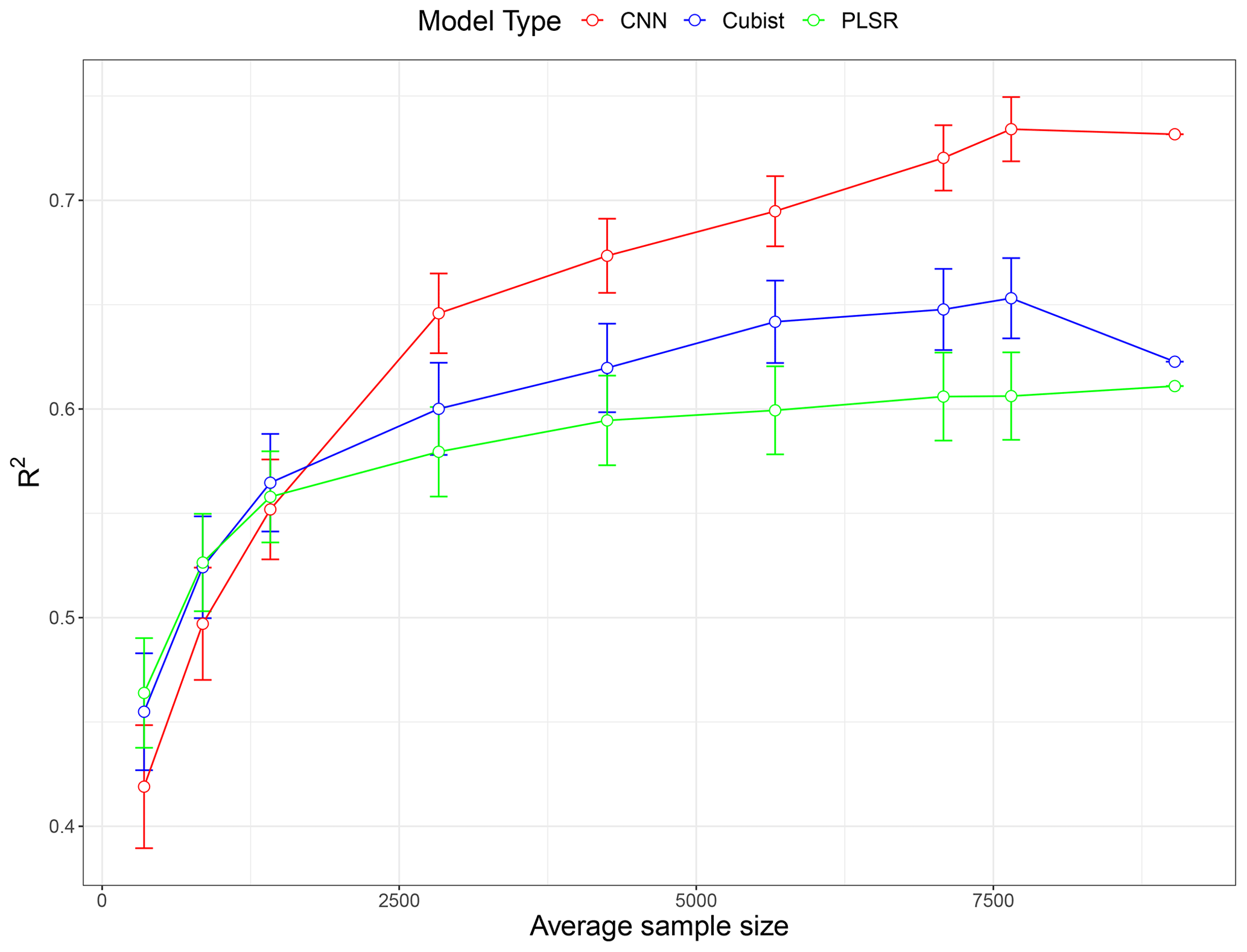
Figure 6Model performances (in terms of average R2 for five soil properties) as a function of sample size using partial least squares regression (PLSR), Cubist and convolutional neural network (CNN) models based on 10 simulations. The value for the largest sample size (N=9027) is a single realisation 75 % of the data.
In general, the PLSR and Cubist models tended to perform better when the sample size was relatively small (<1500). When the sample size was approximately 1800, there was only a small difference in the performances for all models. However, when the sample size was further increased (>2000), the CNN model started to show a better performance in comparison to both PLSR and Cubist models. The effectiveness of PLSR and Cubist models reached a plateau at approximately 4000 and 5500 samples, respectively, while the performance of CNN was still increasing, as depicted in the theoretical curve (Fig. 1). The slight drop in Cubist's performance at sample size 9027 was because there was only one realisation of data split (75 % of the data).
We further compared the average model performance based on the RMSE ratios of machine learning models against the CNN model (Fig. 7). This comparison was developed using the model performance for each unique property, and the variances presented were based on 10 simulations. If a particular X model performs better than the Y model it is compared against, then the RMSE ratios of X ∕ Y should be less than one.
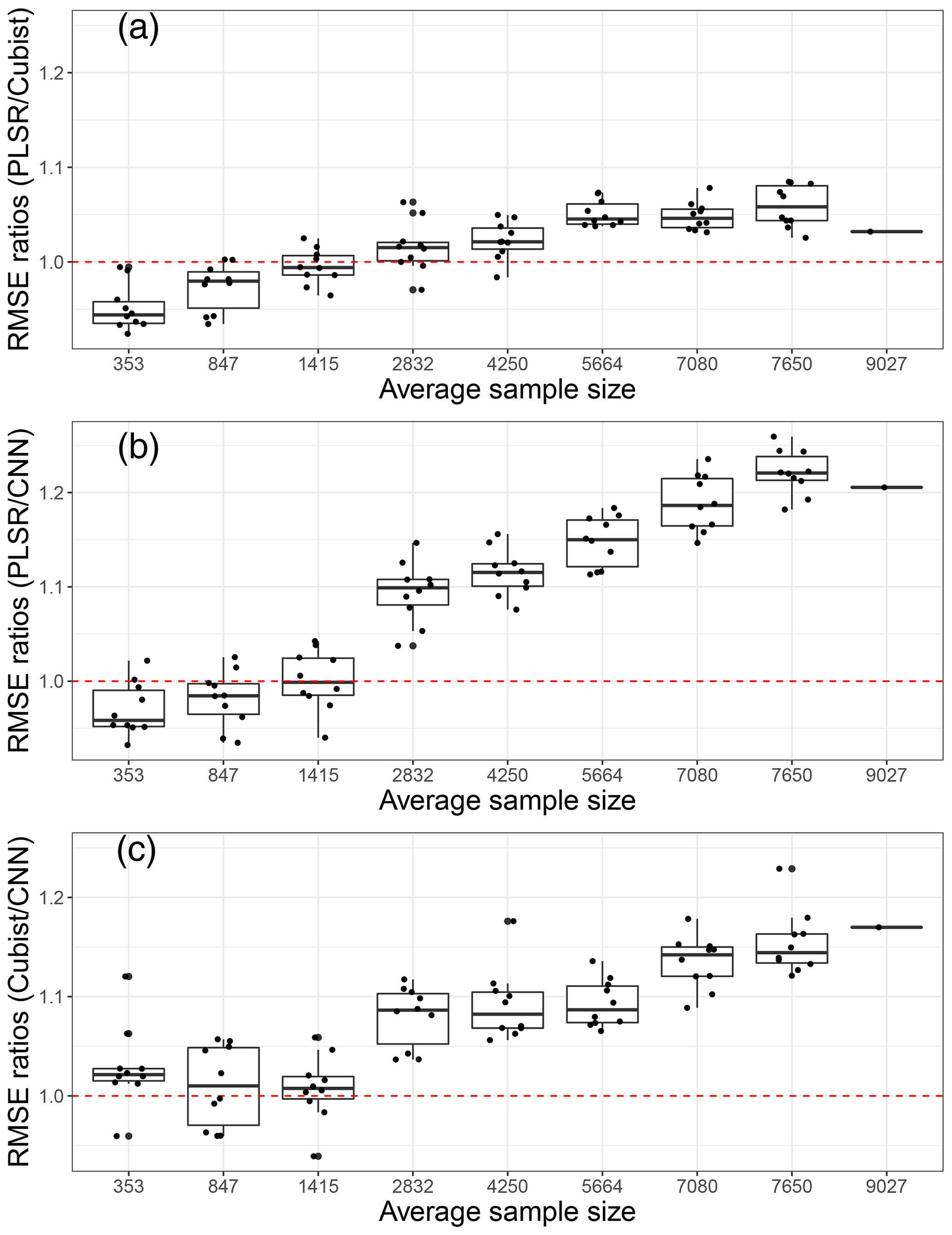
Figure 7Model performances in terms of root mean square error (RMSE) ratios of (a) partial least squares regression (PLSR) over Cubist model, (b) PLSR over convolutional neural network (CNN) model and (c) Cubist over CNN as an average of five soil properties, based on various sample size using 10 simulations. The red dotted line represents a 1 : 1 RMSE ratio.
Upon comparing the RMSE ratios of the PLSR and Cubist models, we found that PLSR performed better than the Cubist model when the sample size was less than 1400. The Cubist model performed better than the PLSR model as the sample size was increased. Using the RMSE ratios of PLSR and CNN models, PLSR was found to perform better than CNN when the sample was less than 1400 (Fig. 7). Similar performance of both PLSR and CNN models was achieved when the sample size was approximately 1400. In terms of RMSE ratios of Cubist and CNN, the CNN model performed better overall in comparison to the Cubist model, regardless of sample size. This was slightly different to the one that was observed when only the R2 parameter was utilised. The RMSE ratios of Cubist and CNN models seemed to vary more for a smaller sample size (longer whisker). When the sample size is approximately 850, both models seemed to perform similarly. A portion of the model performed better, while the remainder performed worse. As the calibration sample size increased, the CNN model performed better in comparison to the Cubist model. Thus, it can be recommended that the current CNN model structure is most efficient for VIS–NIR–SWIR spectra modelling with sample sizes above 2000. CNN can still be used for a small number of samples, but its performance is not better than PLSR or Cubist.
3.5 Sensitivity analysis
The critique of CNN is that it is a complex model and a black box. To uncover how the CNN model works, a sensitivity analysis was conducted to show how CNN predicts each of the soil properties, as illustrated in Fig. 8. Only certain parts of the spectra were used by the CNN model for prediction, which corresponded to the soil properties and composition. The important wavelengths for the prediction of CEC are between the regions of 1600 and 2000 nm. This result is similar to the observations made by Lee et al. (2009) on the surface horizon data set, where 1772 and 1805 nm are essential for predicting the CEC. The presence of high CEC is often linked to the presence of OC and clay content. It is interesting that the same region is important for predicting organic carbon but not clay content. Aside from the same region used by CEC, the wavelengths' region between 1100 and 1200 nm is also deemed relevant by the CNN model for the prediction of OC content. This finding is slightly different to those reported by Lee et al. (2009) in which the important wavelengths reported are at 1772, 1871, 2069, 2246, 2351 and 2483 nm for the profile data set and 1871, 2072 and 2177 nm for the surface horizon data set.

Figure 8Sensitivity analysis of the visible, near and shortwave infrared (VIS–NIR–SWIR) spectra in predicting various soil properties using the convolutional neural network (CNN) model. The graph depicts the sensitivity index (calculated from Eq. 2) for different soil properties as a function of wavelength.
Similar wavelength regions are deemed to be important for predicting the soil texture, although the importance varied slightly among the types of texture of interest (sand, silt and clay) at wavelengths between 500 and 1800 nm. The important wavelengths for the prediction of sand and clay content share a higher similarity in comparison to those of silt content prediction. The most crucial wavelength identified is around 850 nm for the prediction of sand and clay content and around 1100 nm for the prediction of silt content. These observations are also different from those reported by Demattê (2002) and Lee et al. (2009), where the important wavelengths for the prediction of soil texture are at 1800–2400 nm. In particular, the soil texture prediction found in the CNN model is strongly related to hematite and/or goethite, -OH and Al–OH groups from kaolinite (Viscarra Rossel and Behrens, 2010; Pinheiro et al., 2017; Fang et al., 2018).
We also compare important wavelengths from the machine learning models against the one from the deep learning model for the prediction of OC, as an example. Common wavelengths found to be related to the organic carbon predictions are 1100, 1600, 1700–1800, 2000 and 2200–2400 nm (Dalal and Henry, 1986; Stenberg et al., 2010).
As a comparison, we calculated important wavelengths used in the PLSR and Cubist models. The important wavelengths utilised in the PLSR model were derived based on the absolute value of the regression coefficients. The height of the line indicates the importance of particular wavelengths for the determination of organic carbon content in the soil. Important wavelengths identified for the prediction of organic carbon were 500–700, 1400 and 1715 nm.
The wavelengths used in the Cubist model were derived based on model usage, either as predictors (blue lines) or conditions (pink lines) (Fig. 9). Some of the wavelengths used in the Cubist model are similar to those observed in the PLSR model, particularly the visible (500–700 nm) and shortwave infrared regions (1400 and 1900 nm).
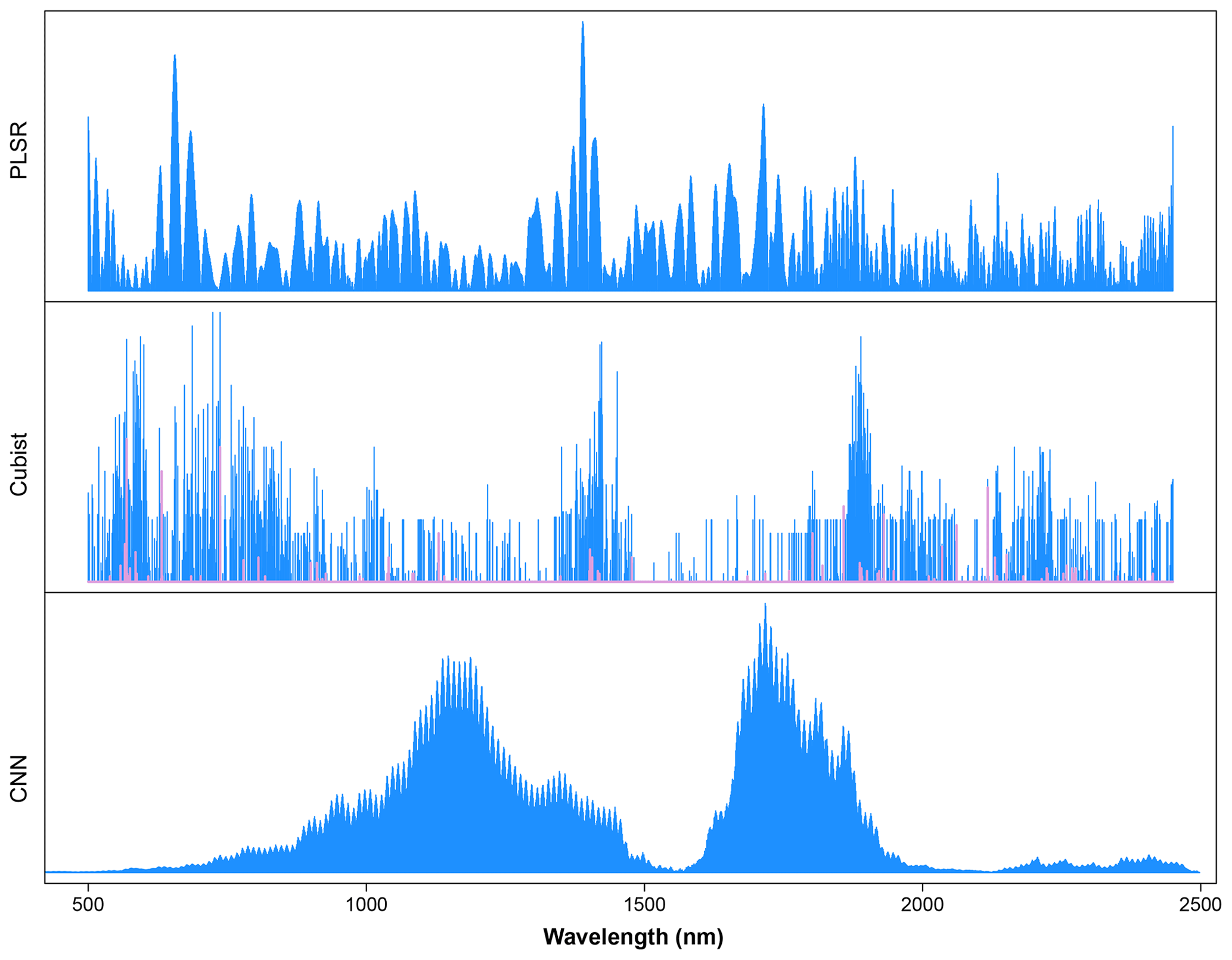
Figure 9Important wavelengths for the prediction of organic carbon (OC) content using partial least squares regression (PLSR), Cubist and convolutional neural network (CNN) models.
4.1 Understanding the CNN models
While conventional PLSR and machine learning models require preprocessing for the spectra input, the CNN model takes raw spectra as inputs. CNN has been shown to be a successful end-to-end learning model which learns feature automatically while minimising hand-crafted preprocessing processes. Upon taking a closer look at the various filters within the convolutional layers, we found that the filters behaved like spectral preprocessing methods. It is interesting to note that, using the raw spectra input, various spectral preprocessing that was commonly used within spectroscopy could be observed within the layer itself. Given the various complexities within the CNN model, the use of spectral preprocessing prior to being fed is unnecessary. This advantage opens up possibilities for developing a highly accurate chemometrics model, which also plays a role in automatic spectral preprocessing.
CNN has been proven to be extremely successful; however, how it works remains largely a mystery as it are buried in layers of computations (Tsakiridis et al., 2020). Sensitivity analysis enabled us to see the inner workings of the CNN model better. We could better understand which wavelength's features are essential to the spectra when used in developing the regression prediction. Important wavelengths derived from the sensitivity analysis based on the CNN model looked slightly different from those of the PLSR and Cubist models. Wavelengths around the 1700 nm region were deemed to be the most important, followed by those in the 1150 nm region. Nonetheless, some of the important regions overlapped. It is also worth noting that the model did not use the visible part of the spectra for prediction. In comparison to the sensitivity of MIR spectra in a previous study (Ng et al., 2019), the NIR model's sensitivity index was much broader, which reflected NIR's characteristic broad peak.
Although all three methods used different ways to derive important wavelengths, the PLSR model tended to use most parts of the spectra. When irrelevant wavelengths are included in model development, it may reduce the model performance. The Cubist model seemed more selective in terms of wavelengths used; however, this example showed that it also used most parts of the VIS–NIR–SWIR spectra. The CNN model used wavelengths between 800 and 2000 nm, with emphasis at around 1100 and 1700 nm.
4.2 The effect of calibration sample size to model performance
PLSR, Cubist and CNN represent models with increased complexity. By combining results from five soil properties, we can better show a generalisation of the performance of the models as a function of training sample sizes. Simpler models (PLSR) performed better at a smaller sample sizes (<1400). Cubist outperformed PLSR at sample sizes >2000, while CNN outweighed other models when sample sizes were >2500. The increase in the accuracy of machine learning models (PLSR and Cubist) became insignificant when the number of samples was greater than 5000. This trend of the plateauing of the performance (maximised up to a certain point) with an increase in sample size has been observed by several authors (Shepherd and Walsh, 2002; Kuang and Mouazen, 2012; Ramirez-Lopez et al., 2014; Ng et al., 2018). This trend is related to the complexity of the model, as a simpler model (such as PLSR) cannot capture all the variations in the data. Thus, a more complex model is suitable when the number of samples is large.
Previous studies by Ng et al. (2019) and Padarian et al. (2019) showed that CNN performed better than PLSR and Cubist when the model was trained with more than 10 000 samples. However, there were also studies using CNN with a small number of training samples. This study showed that the CNN model only outperformed PLSR and Cubist models when the sample size was greater than 2000. As the sample size increases, so the efficiency of the CNN model is increased. We observed a larger reduction in RMSE (CNN compared to the other two models) with an increasing calibration sample size. Thus, we recommend using a minimum of 2000 samples to train the CNN model for the VIS–NIR–SWIR spectra. To further improve the performance of the CNN model, simultaneous prediction of soil properties could also be implemented within the model.
The advantage of using deep learning on a small number of samples is minimal, as CNN is a data-hungry model; it is also more computationally expensive than the typical machine learning models. While our results pertain to the spectra set from Brazil and a particular structure of the CNN, we believe our results can serve as a guide for the number of samples needed to create a better deep learning model. Future research could test this idea on larger and more variable data sets (e.g. a global spectra library with more than 100 000 samples) to see if a more complex and deeper network of CNN can handle such data set.
We assessed the effect of the training sample size and identified important wavelengths in predicting various soil properties using Cubist and CNN models. Here, we found that, with its current model structure, CNN is more accurate than machine learning models when the number of calibration samples is above 2000. The more complex and deeper the network of a deep learning model, the more likely it will need a larger number of samples for training. PLSR and Cubist models perform less accurately than the CNN model as sample size increases, and both models reached a plateau after a sample size of 4000–5000. Meanwhile, the performance of CNN still increased until the maximum number of data used in this study (N=9000) was reached. Future studies should explore larger data sets to test the generalisation of the accuracy vs. sample size and to explore if the deep learning CNN model ever reaches a plateau in accuracy.
Data are courtesy of Dematte; they are not publicly accessible as they were taken from private farms.
WN was responsible for the data analysis and prepared the paper. BM contributed to the idea, data analysis and editing the paper. WdSM and JAMD contributed to the idea, provided the data and assisted with the editing of the paper.
The authors declare that they have no conflict of interest.
This study was supported in part by the Australian Research Council (ARC) Linkage Project (grant no. LP150100566) on the optimised field delineation of contaminated soils. The authors would also like to thank members of the Geotechnologies in Soil Science Group (https://esalqgeocis.wixsite.com/geocis, last access: 1 July 2019). Budiman Minasny is a member of the GLADSOILMAP consortium supported by LE STUDIUM Loire Valley Institute for Advanced Studies through its LE STUDIUM Research Consortium Programme.
This research has been supported by the ARC Linkage Project (grant no. LP150100566) and the São Paulo Research Foundation (FAPESP; grant nos. 2014/22262-0 and 2016/26124-6).
This paper was edited by Bas van Wesemael and reviewed by three anonymous referees.
Acquarelli, J., van Laarhoven, T., Gerretzen, J., Tran, T. N., Buydens, L. M. C., and Marchiori, E.: Convolutional neural networks for vibrational spectroscopic data analysis, Anal. Chim. Acta, 954, 22–31, https://doi.org/10.1016/j.aca.2016.12.010, 2017.
Abadi, M., Barham, P., Chen, J., Chen, Z., Davis, A., Dean, J., Devin, M., Ghemawat, S., Irving, G., Isard, M., Kudlur, M., Levenberg, J., Monga, R., Moore, S., Murray, D. G., Steiner, B., Tucker, P., Vasudevan, V., Warden, P., Wicke, M., Yu, Y., and Zheng, X.: TensorFlow: Large-scale machine learning on heterogeneous systems, Software available from tensorflow.org, available at: https://www.tensorflow.org/ (last access: 1 July 2019), 2015.
Barnes, R. J., Dhanoa, M. S., and Lister, S. J.: Standard Normal Variate Transformation and De-Trending of near-Infrared Diffuse Reflectance Spectra, Appl. Spectrosc., 43, 772–777, https://doi.org/10.1366/0003702894202201, 1989.
Bellinaso, H., Demattê, J. A. M., and Romeiro, S. A.: Soil Spectral Library and Its Use in Soil Classification, Rev. Bras. Cienc. Solo, 34, 861–870, https://doi.org/10.1590/S0100-06832010000300027, 2010.
Bendor, E. and Banin, A.: Near-Infrared Analysis as a Rapid Method to Simultaneously Evaluate Several Soil Properties, Soil Sci. Soc. Am. J., 59, 364–372, https://doi.org/10.2136/sssaj1995.03615995005900020014x, 1995.
Chang, C. W., Laird, D. A., Mausbach, M. J., and Hurburgh, C. R.: Near-infrared reflectance spectroscopy-principal components regression analyses of soil properties, Soil Sci. Soc. Am. J., 65, 480–490, 2001.
Chen, H. Z., Liu, Z. Y., Gu, J., Ai, W., Wen, J. B., and Cai, K.: Quantitative analysis of soil nutrition based on FT-NIR spectroscopy integrated with BP neural deep learning, Anal. Methods-UK, 10, 5004–5013, https://doi.org/10.1039/c8ay01076e, 2018.
Chollet, F.: Keras, available at: https://github.com/fchollet/keras (last access: 1 July 2019), 2015.
Clark, R. N.: Chapter 1: Spectroscopy of Rocks and Minerals, and Principles of Spectroscopy, in: Manual of Remote Sensing, edited by: Rencz, A. N., Remote Sensing for the Earth Sciences, John Wiley and Sons, New York, 3–58, 1999.
Cui, C. H. and Fearn, T.: Modern practical convolutional neural networks for multivariate regression: Applications to NIR calibration, Chemometr. Intell. Lab., 182, 9–20, https://doi.org/10.1016/j.chemolab.2018.07.008, 2018.
Dalal, R. C. and Henry, R. J.: Simultaneous Determination of Moisture, Organic-Carbon, and Total Nitrogen by near-Infrared Reflectance Spectrophotometry, Soil Sci. Soc. Am. J., 50, 120–123, https://doi.org/10.2136/sssaj1986.03615995005000010023x, 1986.
Dangal, S., Sanderman, J., Wills, S., and Ramirez-Lopez, L.: Accurate and Precise Prediction of Soil Properties from a Large Mid-Infrared Spectral Library, Soil Systems, 3, 11, https://doi.org/10.3390/soilsystems3010011, 2019.
Demattê, J. A. M.: Characterization and discrimination of soils by their reflected electromagnetic energy, Pesqui. Agropecu. Bras., 37, 1445–1458, https://doi.org/10.1590/S0100-204x2002001000013, 2002.
Demattê, J. A. M., Bellinaso, H., Araujo, S. R., Rizzo, R., and Souza, A. B.: Spectral regionalization of tropical soils in the estimation of soil attributes, Rev. Cienc. Agron., 47, 589–598, 2016.
Donagema, G. K., de Campos, D. B., Calderano, S. B., Teixeira, W., and Viana, J. M.: Manual de métodos de análise de solo, Embrapa Solos-Documentos (INFOTECA-E), 2011.
Fang, Q., Hanlie, H., Zhao, L., Kukolich, S., Yin, K., and Wang, C.: Visible and near-infrared reflectance spectroscopy for investigating soil mineralogy, 2018, https://doi.org/10.1155/2018/3168974, 2018.
Figueroa, R. L., Zeng-Treitler, Q., Kandula, S., and Ngo, L. H.: Predicting sample size required for classification performance, BMC Med. Inform. Decis., 12, 8, https://doi.org/10.1186/1472-6947-12-8, 2012.
He, K. M., Zhang, X. Y., Ren, S. Q., and Sun, J.: Deep Residual Learning for Image Recognition, 2016 Ieee Conference on Computer Vision and Pattern Recognition (Cvpr), IEEE, 770–778, https://doi.org/10.1109/Cvpr.2016.90, 2016.
Islam, K., Singh, B., and McBratney, A.: Simultaneous estimation of several soil properties by ultra-violet, visible, and near-infrared reflectance spectroscopy, Aust. J. Soil Res., 41, 1101–1114, https://doi.org/10.1071/Sr02137, 2003.
Kingma, D. P. and Ba, J.: Adam: A method for stochastic optimization, arXiv [preprint], arXiv:1412.6980, 2014.
Krizhevsky, A., Sutskever, I., and Hinton, G. E.: ImageNet classification with deep convolutional neural networks, Proceedings of the 25th International Conference on Neural Information Processing Systems – Volume 1, Lake Tahoe, Nevada, New York: Curran Associates, Inc., 2012.
Kuang, B. and Mouazen, A. M.: Influence of the number of samples on prediction error of visible and near infrared spectroscopy of selected soil properties at the farm scale, Eur. J. Soil Sci., 63, 421–429, https://doi.org/10.1111/j.1365-2389.2012.01456.x, 2012.
Kuhn, M. and Quinlan, R.: Cubist: Rule- And Instance-Based Regression Modeling, R package version 0.2.2, available at: https://CRAN.R-project.org/package=Cubist (last access: 18 July 2019), 2018.
LeCun, Y., Bengio, Y., and Hinton, G.: Deep learning, Nature, 521, 436–444, https://doi.org/10.1038/nature14539, 2015.
Lee, K. S., Lee, D. H., Sudduth, K. A., Chung, S. O., Kitchen, N. R., and Drummond, S. T.: Wavelength Identification and Diffuse Reflectance Estimation for Surface and Profile Soil Properties, T. ASABE, 52, 683–695, 2009.
Liu, L., Ji, M., and Buchroithner, M.: Transfer Learning for Soil Spectroscopy Based on Convolutional Neural Networks and Its Application in Soil Clay Content Mapping Using Hyperspectral Imagery, Sensors-Basel, 18, https://doi.org/10.3390/s18093169, 2018.
Mahapatra, S.: Why Deep Learning over Traditional Machine Learning?, available at: https://towardsdatascience.com/why-deep-learning-is-needed-over-traditional-machine-learning-1b6a99177063 (last access: 1 July 2019), 2018.
Mevik, B.-H., Wehrens, R., and Liland, K. H.: pls: Partial Least Squares and Principal Component Regression. R package version 2.7-0, available at: https://CRAN.R-project.org/package=pls (last access: 18 July 2019), 2018.
Ng, W., Minasny, B., Malone, B., and Filippi, P.: In search of an optimum sampling algorithm for prediction of soil properties from infrared spectra, PeerJ, 6, e5722, https://doi.org/10.7717/peerj.5722, 2018.
Ng, W., Minasny, B., Montazerolghaem, M., Padarian, J., Ferguson, R., Bailey, S., and McBratney, A. B.: Convolutional neural network for simultaneous prediction of several soil properties using visible/near-infrared, mid-infrared, and their combined spectra, Geoderma, 352, 251–267, https://doi.org/10.1016/j.geoderma.2019.06.016, 2019.
Padarian, J., Minasny, B., and McBratney, A. B.: Using deep learning to predict soil properties from regional spectral data, Geoderma Regional, 16, e00198, https://doi.org/10.1016/j.geodrs.2018.e00198, 2019.
Pinheiro, E. F. M., Ceddia, M. B., Clingensmith, C. M., Grunwald, S., and Vasques, G. M.: Prediction of Soil Physical and Chemical Properties by Visible and Near-Infrared Diffuse Reflectance Spectroscopy in the Central Amazon, Remote Sens-Basel, 9, 293, https://doi.org/10.3390/rs9040293, 2017.
Python Software Foundation: Python Language Reference, Python Software Foundation, available at: https://www.python.org (last access: 1 July 2019), 2017.
Quinlan, J. R.: C4.5: Programs for Machine Learning, Morgan Kaufmann Publishers Inc., San Mateo, California, 1993.
R Core Team: R: A language and environment for statistical computing, available at: https://www.R-project.org/ (last access: 18 July 2019), 2019.
Ramirez-Lopez, L., Schmidt, K., Behrens, T., van Wesemael, B., Dematte, J. A. M., and Scholten, T.: Sampling optimal calibration sets in soil infrared spectroscopy, Geoderma, 226, 140–150, https://doi.org/10.1016/j.geoderma.2014.02.002, 2014.
Rinnan, A., van den Berg, F., and Engelsen, S. B.: Review of the most common pre-processing techniques for near-infrared spectra, Trac-Trend Anal. Chem., 28, 1201–1222, https://doi.org/10.1016/j.trac.2009.07.007, 2009.
Savitzky, A. and Golay, M. J. E.: Smoothing and Differentiation of Data by Simplified Least Squares Procedures, Anal. Chem., 36, 1627–1639, https://doi.org/10.1021/ac60214a047, 1964.
Shepherd, K. D. and Walsh, M. G.: Development of Reflectance Spectral Libraries for Characterization of Soil Properties, Soil Sci. Soc. Am. J., 66, 988–998, https://doi.org/10.2136/sssaj2002.9880, 2002.
Shibusawa, S., Imade Anom, S. W., Sato, S., Sasao, A., and Hirako, S.: Soil mapping using the real-time soil spectrophotometer, in: ECPA, Third European Conference on Precision Agriculture, edited by: Grenier, G. and Blackmore, S., Agro Montpellier, 1. Montpellier, France, 497–508, 2001.
Simonyan, K. and Zisserman, A.: Very Deep Convolutional Networks for Large-Scale Image Recognition, CoRR, abs/1409.1556, 2014.
Stenberg, B., Viscarra Rossel, R. A., Mouazen, A. M., and Wetterlind, J.: Chapter Five – Visible and Near Infrared Spectroscopy in Soil Science, in: Adv Agron, edited by: Sparks, D. L., Academic Press, Burlington, MA, 163–215, 2010.
Szegedy, C., Liu, W., Jia, Y. Q., Sermanet, P., Reed, S., Anguelov, D., Erhan, D., Vanhoucke, V., and Rabinovich, A.: Going Deeper with Convolutions, Proc. Cvpr Ieee, Piscataway: IEEE, 1–9, 2015.
Terra, F. S., Dematte, J. A. M., and Rossel, R. A. V.: Proximal spectral sensing in pedological assessments: vis-NIR spectra for soil classification based on weathering and pedogenesis, Geoderma, 318, 123–136, https://doi.org/10.1016/j.geoderma.2017.10.053, 2018.
Tsakiridis, N. L., Keramaris, K. D., Theocharis, J. B., and Zalidis, G. C.: Simultaneous prediction of soil properties from VNIR-SWIR spectra using a localized multi-channel 1-D convolutional neural network, Geoderma, 367, 114208, https://doi.org/10.1016/j.geoderma.2020.114208, 2020.
Viscarra Rossel, R. A. and Behrens, T.: Using data mining to model and interpret soil diffuse reflectance spectra, Geoderma, 158, 46–54, https://doi.org/10.1016/j.geoderma.2009.12.025, 2010.
Viscarra Rossel, R. A., Cattle, S. R., Ortega, A., and Fouad, Y.: In situ measurements of soil colour, mineral composition and clay content by vis–NIR spectroscopy, Geoderma, 150, 253–266, https://doi.org/10.1016/j.geoderma.2009.01.025, 2009.
Walkley, A. and Black, I. A.: An examination of the Degtjareff method for determining soil organic matter, and a proposed modification of the chromic acid titration method, Soil Sci., 37, 29–38, https://doi.org/10.1097/00010694-193401000-00003, 1934.
Wold, S., Martens, H., and Wold, H.: The Multivariate Calibration-Problem in Chemistry Solved by the Pls Method, Lect. Notes Math., 973, 286–293, 1983.
Yang, J., Xu, J. F., Zhang, X. L., Wu, C. Y., Lin, T., and Ying, Y. B.: Deep learning for vibrational spectral analysis: Recent progress and a practical guide, Anal. Chim. Acta, 1081, 6–17, https://doi.org/10.1016/j.aca.2019.06.012, 2019.
Zhang, X. L., Xu, J. F., Yang, J., Chen, L., Zhou, H. B., Liu, X. J., Li, H. F., Lin, T., and Ying, Y. B.: Understanding the learning mechanism of convolutional neural networks in spectral analysis, Anal. Chim. Acta, 1119, 41–51, https://doi.org/10.1016/j.aca.2020.03.055, 2020.
Zhu, X., Vondrick, C., Fowlkes, C. C., and Ramanan, D.: Do We Need More Training Data?, International Journal of Computer Vision, 119, 76–92, https://doi.org/10.1007/s11263-015-0812-2, 2016.