Soil environment grouping system based on spectral, climate, and terrain data: a quantitative branch of soil series

Soil classification has traditionally been developed by combining the interpretation of taxonomic rules that are related to soil information with the pedologist's tacit knowledge. Hence, a more quantitative approach is necessary to characterize soils with less subjectivity. The objective of this study was to develop a soil grouping system based on spectral, climate, and terrain variables with the aim of establishing a quantitative way of classifying soils. Spectral data were utilized to obtain information about the soil, and this information was complemented by climate and terrain variables in order to simulate the pedologist knowledge of soil–environment interactions. We used a data set of 2287 soil profiles from five Brazilian regions. The soil classes of World Reference Base (WRB) system were predicted using the three above-mentioned variables, and the results showed that they were able to correctly classify the soils with an overall accuracy of 88 %. To derive the new system, we applied the spectral, climatic, and terrain variables, which – using cluster analysis – defined eight groups; thus, these groups were not generated by the traditional taxonomic method but instead by grouping areas with similar characteristics expressed by the variables indicated. They were denominated as “soil environment groupings” (SEGs). The SEG system facilitated the identification of groups with equivalent characteristics using not only soil but also environmental variables for their distinction. Finally, the conceptual characteristics of the eight SEGs were described. The new system has been designed to incorporate applicable soil data for agricultural management, to require less interference from personal/subjective/empirical knowledge (which is an issue in traditional taxonomic systems), and to provide more reliable automated measurements using sensors.

1 Introduction

Knowledge regarding soil has gained importance since humans learnt to cultivate the land about 10 000 years ago. The experience gained over this period must be converted into applied knowledge to solve modern issues involving the soil. In this respect, pedology plays a fundamental role in the understanding of soil formation factors and their spatial distribution. The pedologist uses their tacit and empirical knowledge to represent the soil using names. This nomenclature is performed based on a taxonomic classification system with several rules. Soil classification nomenclature has traditionally been achieved by combining the interpretation of soil properties; soil–landscape relations, with the support of maps, aerial or satellite images; and the pedologist's knowledge on soils (Demattê and Terra, 2014). The formative elements of most soil classes' nomenclature do not consider climate or terrain data, which are important factors in soil formation. Therefore, there often seems to be no coherence, and comparison is impaired when we try to associate the name of the soil with the landscape. This occurs due to two factors: (a) the pedologist's knowledge is inherent, acquired with years of learning (which demands time), and is extremely difficult to extract in a quantitative way; and (b) the pedologist has to follow taxonomic rules. As an alternative, we need to seek sources that aggregate the soil–landscape information into a classification system.

One source of soil–landscape features is remote sensing (RS) images. Over the last few decades, RS has gradually been applied in a more quantitative way to the interpretation of soil classes (Demattê et al., 2004; Mulder et al., 2011; Teng et al., 2018; Viscarra Rossel et al., 2016). Using digital elevation models, it is possible to extract several terrain attributes that can then be taken into consideration by a pedologist in a soil survey (Florinsky, 2012). In addition, the climate can contribute to a general understanding of the soil (Brevik et al., 2018) and can also assist in its quantification depending on the scale of the study. Climate plays a fundamental role in weathering and soil formation, while the terrain attributes greatly influence the soil genesis. Thus, these variables are an essential allies in the search for a better grouping and comprehension of the soil.

Another issue is that traditional soil classification data are becoming increasingly challenging to obtain due to the reliance on pedologists' knowledge. Moreover, the complexity and the large number of soil characteristics that should be considered in order to classify the soil profile are another complication. The information about soil classification is becoming scarce in soil libraries, and these libraries are avid for quantitative data. As the traditional approach for obtaining soil classification data is insufficient, it is necessary to develop new procedures to acquire soil information in a more measurable way. With the advent of sensors, the collection and determination of soil data from spectral information has become more agile, and, due to advancements in soil research, the data have also become more accurate. Thus, the application of a quantitative technique is necessary to obtain a new system to characterize soils.

This, however, poses the question of how to combine a system that aggregates several soil formation factors without becoming trapped in a taxonomy. From this question, the need for a soil series system emerges. The concept of soil series is based on grouping soils with homogeneous characteristics into a system at the lowest possible level; “soil series” is a common reference term that is used to name soil mapping units. The USDA soil taxonomy (Soil Survey Staff, 2014) is the only classification system hierarchy that has established soil series. The descriptions contain properties that define the soil series and provide a record of the soil properties needed to prepare soil interpretations. Moreover, a soil series is an area that has similar landscape, climate, soil characteristics and, therefore, does not involve taxonomy. As pedology was stuck in taxonomy for years, it has had difficulty creating soil series due to the specificity of this new denomination, in addition to the fear that soil series will not being easily comprehended by the user. However, as almost all surveys today are quantitative, including environmental data, the possibility of a soil series system seems feasible. Therefore, when homogeneous areas are delimited using numerous forms of information regarding the environment, terrain, and soil, the taxonomic nomenclature of the soil classes will no longer be necessary. In this aspect, soil spectroscopy is essential. The soil spectrum carries information about soil characteristics, such as soil organic matter (OM), minerals, texture, nutrients, water, pH, and heavy metals (Stenberg et al., 2010; Viscarra Rossel and McBratney, 2008). Thus, proximal sensing has made significant contributions to soil classification (Viscarra Rossel et al., 2010) and should play a leading role in the development of the new soil series. However, spectral data are limited regarding all of the information needed for soil classification systems. For this reason, environmental data can contribute by supplying the inherent pedologist's knowledge in relation to the soil landscape. Furthermore, the colour, mineralogy, humidity, texture and organic carbon, among other soil properties can be acquired in any part of the world using the same measurement protocol and equipment. Combining this information with climatic and terrain data, it is possible to identify areas with homogeneous characteristics.

The general objective of this study was to create a system that would indicate how to group homogeneous soils based on spectral information and climate, and terrain variables, in order to devise a quantitative method for their classification. We expect that spectral information in combination with climate and terrain data can provide sufficient information for a specific soil to indicate a group, which is more representative than a taxonomic classification system.

2 Material and methods

2.1 Soil data

The soil database consists of 2287 soil profiles from all five regions of Brazil. The data were extracted from the Brazilian Soil Spectral Library (Demattê et al., 2019). The database includes profiles of 10 soil classes, which are classified according to World Reference Base (WRB) – FAO (IUSS, 2015): Arenosol, Cambisol, Ferralsol, Gleysol, Histosol, Lixisol, Luvisol, Nitisol, Planosol, and Regosol. Each soil profile had three depths: A, 0–20 cm; B, 20–60 cm; and C, 60–100 cm. For the statistical analyses, the spectrum of three depths were averaged to compose a single spectrum per profile. In order to balance the number of samples of each soil class, the synthetic minority over-sampling technique (SMOTE) algorithm was applied to avoid imbalance issues in the analyses (Chawla et al., 2002).

2.2 Spectral data

The spectral data were obtained in the Geotechnologies in Soil Science group (GeoCIS), São Paulo, Brazil, using the FieldSpec 3 spectroradiometer (Analytical Spectral Devices – ASD, Boulder, CO). The spectral sensor, which was used to capture light via a fibre optic cable, was located 8 cm from the sample surface. The sensor scanned an area of approximately 2 cm², and a light source was provided by two external 50 W halogen lamps. These lamps were positioned at a distance of 35 cm from the sample (non-collimated rays and a zenithal angle of 30^∘) with an angle of 90^∘ between them. A Spectralon standard white plate was scanned every 20 min during calibration. Two replications (one involving a 180^∘ turn of the Petri dish) were obtained for each sample. Each spectrum was averaged from 100 readings over 10 s. The mean values of the two replicates were used for each sample. The spectral data ranged from the visible to the near-infrared (Vis–NIR) regions (350–2500 nm). The Savitzky–Golay derivative (Savitzky and Golay, 1964) was applied to the spectra with following configuration (polynomial order of 2 and window size of 15). As the spectrum is highly collinear, we only kept the wavelength every 10 nm, resulting in 213 wavelengths for the analysis. The soil colour variables, including hue angle (Ha), value (v), and chroma (c), were derived from the spectrum.

We applied principal component analysis (PCA) to the spectral data to select the scores of the principal components (PC), and we then applied them in the model. The PC eigenvectors were utilized to indicate the wavelengths with the highest contribution in the PCA. The data were not standardized because all of the wavelengths were in the same units and the differences in the variation between them was inherently important. The number of PCs applied in the model was selected in order to capture a high percentage of explained variance and the highest amount of spectral detail possible, as the spectral data present absorption points in different areas of the spectral curve that have distinct intensities.

2.3 Climatic and terrain variables

The climatic and terrain variables applied in the model were extracted from different sources in order to represent the environmental variability. The climatic variables were the potential evapotranspiration (PotEvapoTransp), the soil water balance (SWB), the annual temperature (AnnualTem), and the annual precipitation (AnnualPre). The terrain variables were slope, aspect, hillshade, topographic position index (TPI), terrain ruggedness index (TRI), roughness, and a digital elevation model (DEM). The terrain variables were extracted from the DEM (at a 90 m spatial resolution). Figure 1 shows the locations of the soil sites in Brazil and the variations in the annual temperature.

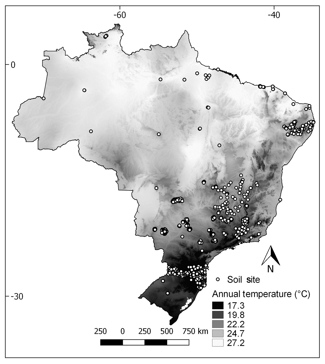
Figure 1 Location of the soil sites (soil data set) in Brazil.

2.4 Supervised modelling to predict soil classes

In order to evaluate the performance of predicting soil classes, we applied a supervised classification method. Random forest (RF) was the algorithm selected, and a 10-fold cross-validation setting was used. In the first modelling approach, only the PCs (derived from the spectra) were applied as independent variables. In the second approach, we added the climatic and terrain variables (to the PCs), and we applied RF to predict the soil classes. The purpose of the second approach was to evaluate the improvement caused by adding climatic and terrain variables to the model. The results were displayed using a confusion matrix and the overall accuracy of the model. From the RF model, we were able to obtain the importance of each variable in the classification.

2.5 Unsupervised modelling for the new classification

To derive the classification system, we needed to select the optimal number of classes. Therefore, unsupervised classification was performed using k-means clustering analysis. In the first approach, we only applied the spectral data in the k-means clustering. Thereafter, we added the climatic and terrain variables to the spectral data and performed the k-means clustering again. Using this procedure, we were able to explore the advantages/disadvantages of adding climate and terrain data to aggregate the groups. To determine how many clusters best described the data, i.e. the optimal number of clusters, the Akaike information criterion (AIC) was utilized. To calculate the AIC, we applied the “kmeansAIC” function from the “kmeansstep” R package. This function calculates the AIC value of a specific k-means cluster and specifies centroids. The AIC was implemented using 1 to 15 clusters. The data-driven analysis was performed 30 times. The overall model number of cluster with the lowest AIC value was selected and was assumed to be the optimal number of clusters, which, in turn, represented the most appropriate number of spectral classes.

2.6 Soil environmental classification

The optimal number of clusters, established using the k-means clustering analysis, was referred to as soil environment groupings (SEGs). The association between traditional soil classes (WRB) and the SEGs was shown by projecting the discriminant coordinates. This procedure allowed one to identify the homogeneity of the classes as well as the proximity of the classes and the relation between them. The correlation between the soil classification and SEGs was arranged in a table. The characterization of each SEG was performed using PCA to evaluate the relationship between the categorical variables, including soil, climate, and terrain variables. The spectral curves for each SEG were represented by averaging the soils classified into the same class.

3 Results

3.1 Extracting the principal components of the spectral data

Discrimination by PCA revealed that the first 10 PCs accounted for 94.5 % of the variance (Fig. A1 in Appendix A). In order to capture the maximum variation in the spectral data, the first 10 PCs were used as the spectral information to predict the traditional soil classification and to develop the SEGs. Vasques et al. (2014) applied 20 PCs to derive the classification models. The eigenvectors of PC1–PC10 represent the important spectral features and the contributions of the absorbance at individual wavelengths (Fig. A2). According to Viscarra Rossel and Webster (2011), the functional groups of minerals and organic components that were most useful in the discrimination of soil classes were those related to iron oxides (hematite and goethite; 430, 495, and 570 nm), O–H–O in 2 : 1 clay minerals (illite and smectite; 1420 and 1900 nm), organics and clay minerals (2150 nm), and Al–OH clay minerals (gibbsite; 2250 nm). The wavelengths for these absorption peaks are approximate. According to Bishop et al. (2008), these peaks may shift from the expected wavelengths because real molecules do not behave totally harmonically when they vibrate and/or due to differences in the measurement conditions and instrumentation.

3.2 Predicting traditional soil classes

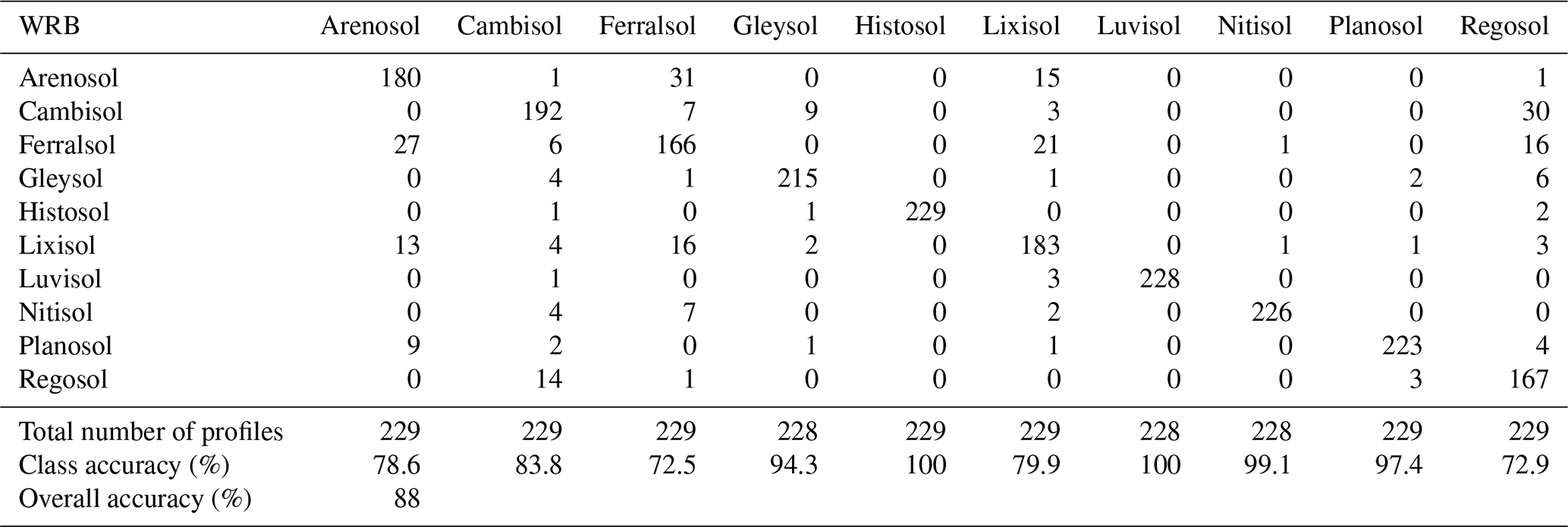
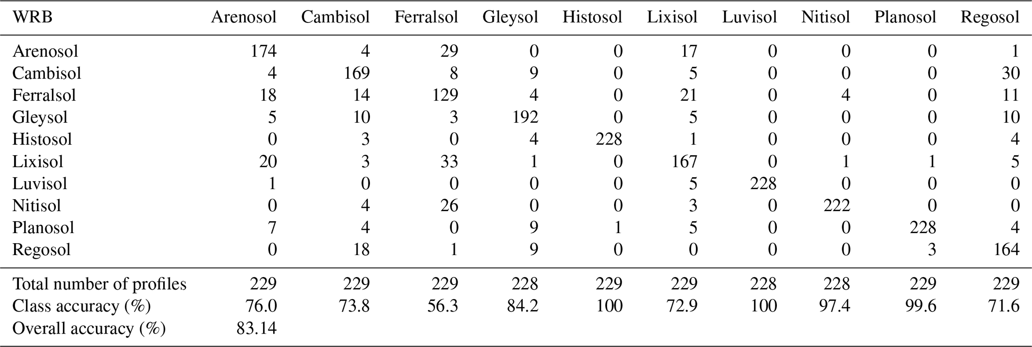
The performance of the RF model showed an overall accuracy of 83 % using spectral data alone (Table A1 in Appendix A). The confusion matrix and the accuracy of the RF analysis including spectral, climatic, and terrain variables are shown in Table 1. The overall accuracy of this classification model using RF was superior, reaching 88 %. The values in the matrix are the number of samples in each class allocated by the RF model. Three soil classes showed an improvement of 10 % or more in the prediction when climatic and terrain variables were added to the model. The overall accuracy of Cambisol increased from 73.8 % to 83.8 %, Gleysol increased from 84.2 % to 94.3 %, and Ferralsol presented the largest improvement, rising from 56.3 % to 72.5 %. The RF model with spectral, climatic, and terrain data was able to assign the correct soil class with very good accuracy for Histosol, Luvisol, Planosol, Nitisol, and Gleysol, reaching values of over 94.3%. Ferralsol was the most misclassified class, with the accuracy reaching only 72.5 %; consequently, a total of 27.8 % of profiles were reallocated to other classes – mostly to Arenosol (14 %), Lixisol (7 %), and Regosol (3 %), as seen in Table 1. Regosol showed a class accuracy of 72.9 %, with most of its misclassified profiles reallocated to Cambisol (13 %) and Ferralsol (7 %). Cambisol presented relatively moderate class accuracy (83.8 %), with most of the errors reallocated to Regosol (6 %). Both the Cambisol and Regosol classes present similarities: Regosols comprise soils in unconsolidated deposits that show little sign of pedogenesis and have no B horizon, and Cambisols present the beginning of soil formation with weak horizon differentiation. As for Arenosols (which had a class accuracy of 76 %), misclassification was predominantly observed with Ferralsols, Lixisols, and Planosols. Lixisols (which had a class accuracy of 79.9 %) were also misclassified as Ferralsols (9 %) and Arenosols (7 %), indicating that these three classes have common soil properties. Arenosols are soils with little or no profile differentiation with a loamy sand or coarser texture class; the majority of Ferralsols in the current data set contained high sand content; and the same was found for Lixisols. The latter two soil classes presented sandy characteristics because they are predominantly derived from sandstone rocks. Thus, the three above-mentioned classes were not well distinguished by the model. Overall, not all misclassifications were negative as some classes are very similar with respect to their properties and use, although other classes were radically different.

Table 1 Confusion matrix and accuracy of soil classification model (World Reference Base, WRB) using spectral, climatic, and terrain data.

3.3 Variable importance from the soil classification model

The importance of variables derived from the RF model are represented in Fig. 2. The variable importance of the spectral data is represented using 10 PCs. PC1 presented a variable importance of more than 50 % with respect to discriminating almost all of the soil classes, with the exception of Cambisol. PC1 also showed a significant contribution to distinguishing soils with an absorption effect in the visible region (380 to 740 nm), where the characteristics of iron oxide are present (Fig. A2). Furthermore, it exhibited important bands related to hydroxyl bonds (1420 and 1900 nm) and organics and clay mineral peaks (2150 and 2250 nm). The remaining PCs showed important bands related to the same features but with varying intensity. Ferralsols and Nitisols are associated with iron oxides in the visible region of the spectrum, where PC1 showed a high contribution (Fig. A2). Planosols contain a high clay content in the subsurface horizon, which indicates the presence of clay minerals. Histosols are rich in organic minerals, which are presented in PC1 (Fig. A2). These soil classes were those with higher variable importance considering the spectral data (PC1 accounted for 47 % of the variance; Fig. A2). As the variance explained in the PCs decreased, so did their importance in the classification.

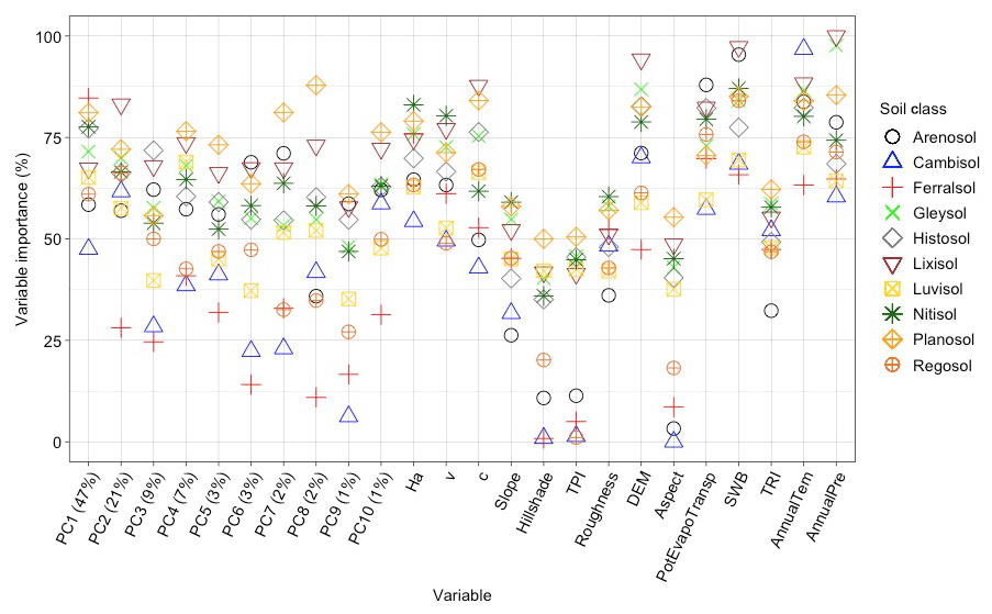
Figure 2 Variable importance for each soil class derived from the model using spectral, climatic, and terrain data.

The soil colour is one of the main soil properties that influences the soil spectral response. The variables expressing the colour characteristics of the soils are Ha, v, and c. The colour, specifically Ha and v, is important to discriminate Nitisols, which are heavy, weathered tropical soils that are red in colour and have a lower overall reflectance. Hillshade, TPI, roughness, aspect, and TRI showed relatively low to medium importance for all of the classes, although they were most significant for distinguishing the Planosols. As Planosols are comprised of impermeable subsoil with significantly more clay in the subsurface horizon and are typically located in seasonally waterlogged flat areas, these terrain variables were able to discriminate them. The DEM showed high importance for Lixisols and low importance for Ferralsols, which indicates that the Ferralsols are located in different sections of the landscape and are not limited to a certain altitude; thus, the high DEM range negatively affected the importance of this variable with respect to predicting Ferralsols. PotEvapoTransp was most important for Arenosols: as this soil class has a high sand content, especially in the surface horizon, the PotEvapoTransp is elevated, which contributed to their discrimination. SWB was an important variable with respect to discriminating Lixisols and Arenosols. Lixisols are soils with a subsurface accumulation of low-activity clay and a high base saturation, which means that they are moderately drained (due to the argic horizon); thus, they may present a low water retention capacity. SWB refers to the amount of water held in the soil. Because Lixisols are soils that can hold a limited amount of water, there is a risk of percolation at depth or runoff under high precipitation conditions. For Arenosols, the high content of the sand fraction throughout the profile contributed to a high importance of SWB with respect to predicting this class. The temperature was important to discriminate Cambisols, as these soils were mostly located in the south and southeast regions of Brazil, where the average annual temperature is low. The annual precipitation was an important variable for Lixisols and Gleysols, as high precipitation is associated with a high soil moisture content, and these two soils have an impermeable subsurface horizon condition, superficial water retention, and, consequently, high soil moisture.

3.4 Developing the soil environmental classification

The lowest AIC value was found with eight clusters (Fig. A3), which represent the best spectra categorization. This means that the optimal number of cluster for the current data set is eight. Subsequently, the k-means clustering was performed using an unsupervised classification method applying eight groups. Firstly, the discriminant coordinate projection, from the clustering analysis using only the spectral data, showed the distribution of the eight SEGs (Fig. 3). The soil classes located on the left side of Fig. 3 were soils with less weathering, such as Histosols and Regosols (far left) followed by Planosols, Gleysols, and Cambisols. On the right side of Fig. 3, we find Ferralsols and Nitisols, which are the more weathered soils. In general, the intermediately weathered soils, such as Luvisols, Lixisols, and Arenosols were located in the centre. This tendency proves that the spectral data were able to discriminate between soils in different stages of weathering. Arenosols can be considered as soils with a low level of weathering. However, in the Fig. 3, they were close to the Ferralsol and Nitisol classes (Fig. 3). This occurred because both Arenosols and Ferralsols have high sand contents; thus, the spectral curves of both soil classes present soil properties with high similarities.

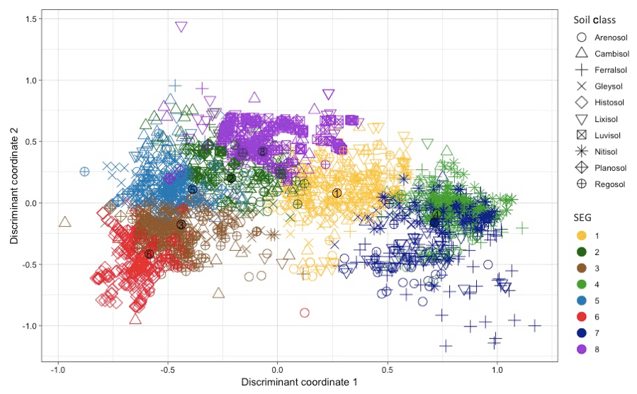
Figure 3 Projection of the discriminant coordinates showing the soil classification and soil environment groupings (SEGs) applying only spectral data for all samples. The circle with the number inside it represents the centre of the SEG.

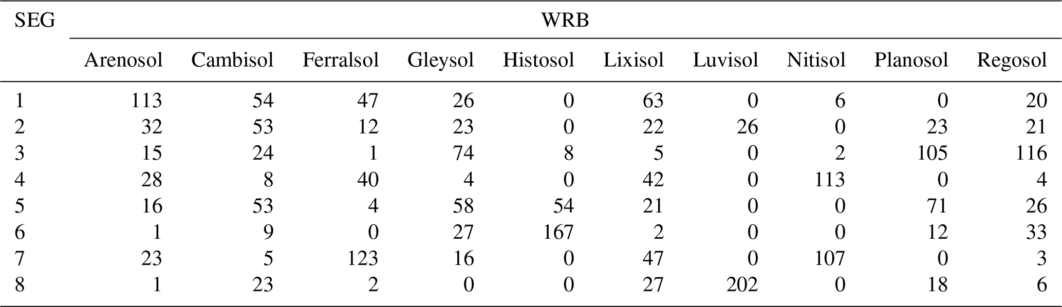
Because the number of soil classes is greater than the number of SEGs, it is expected that some soil classes will be allocated in the same SEGs. The association between the traditional soil classes and the SEGs is shown in Table 2. Arenosols showed the highest correspondence with SEG 1. SEG 2 was associated with Cambisols. SEG 3 was associated with Regosols, Planosols, and Gleysols. SEG 4 presented high correspondence with Nitisols. SEG 5 had a high equivalence with Planosols followed by the Gleysols. SEG 6 was highly correlated with Histosols. SEG 7 was correlated with Ferralsols, although a great quantity of Nitisol samples was also correlated with this SEG. Lastly, SEG 8 presented the highest correspondence with Luvisols. Lixisols did not have a predominant SEG, although they were associated with SEG 1. SEG 3 and 5 were associated with the Regosol, Planosol, and Gleysol soil classes. SEG 4 and 7 also displayed a correlation but, in this case, only with Ferralsols and Nitisols.

Table 2 Correlation between soil classification (World Reference Base, WRB) and soil environment grouping (SEG) using only spectral data.

Subsequently, the clustering analysis using spectral, climatic, and terrain data was performed. The projection of the discriminant coordinates showed that climate and terrain data revealed that the SEGs were more gathered (Fig. 4) compared with the clustering analysis with only spectral data (Fig. 3). SEG 1 and 3, which mainly corresponded to the Ferralsol, Nitisol, and Lixisol classes, had a more widespread distribution of samples (Fig. 4). This arrangement was also observed in the correlation between soil classes and SEGs using only spectral data (SEG 7, Table 2). Two soils were associated with SEG 2: Luvisols and Planosols (Table 3). SEG 3 showed a correlation with Cambisols and Nitisols. SEG 4 only showed 42 observations, which mostly belonged to Gleysols and a few Histosols. These soils were grouped into a specific SEG because they are found in flat areas with DEM values close to sea level that have a very high annual temperature and precipitation compared with the Gleysols clustered in SEG 6. SEG 5 presented a high correspondence with Arenosols and, as in the analysis with only the spectra, also showed a correlation with Ferralsols (SEG 1, Table 2). SEG 6 showed a high association with Gleysols. SEG 7 was formed by Histosols, and SEG 8 was made up of Regosols. The climate and terrain variables were able to better discriminate SEGs, although some soils were located far from the centre of the class. These may have had similar properties to other groups but were not similar enough to fit into them.

Table 3 Correlation between soil classification (World Reference Base, WRB) and soil environment groupings (SEGs) using spectral, climatic, and terrain data.

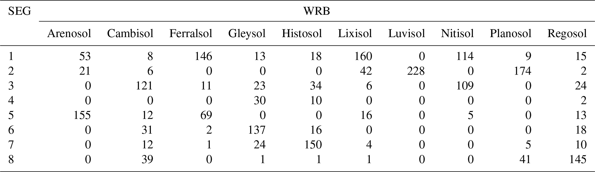
Figure 4 Projection of the discriminant coordinates showing the soil classification (World Reference Base, WRB) and soil environment groupings (SEGs) applying spectral, climatic, and terrain data. The circles with the numbers in them represent the centre of the SEGs.

4 Discussion

Vis–NIR spectroscopy is a technique that has the advantage of being faster and cheaper than the traditional soil analysis, and it enables important soil classification prediction to be acquired in situ (Debaene et al., 2017). Teng et al. (2018) demonstrated the benefit of the technique by updating the Australian Soil Classification with spectroscopic predictions that showed similar or better correspondence for some classes. In this study, the 10 PCs carried sufficient spectral information to suitably classify the soil – as indicated by the overall accuracy of 83 % for the RF calibration model. Vasques et al. (2014) applied 20 PCs in their study to classify the soil orders, and they achieved an overall accuracy of 91.6 % and 67.4 % for calibration and validation respectively. The prediction of traditional soil classes applying only spectral data in this study is considered excellent prediction performance. However, when we added climatic and terrain data into the calibration model (which are utilized as complementary data with the objective of incorporating the pedologist's impersonal knowledge on environmental factors) an improvement in the prediction of soil classes is observed (overall accuracy of 88 %). This result shows that aggregating soil–landscape information into a classification system assists the traditional soil system. Depending on the size of the study area and the characteristics of the study, such an addition may not be beneficial, as climatic and terrain data are time-consuming to assemble and are not practical in a sense. Chen et al. (2019) verified the potential of adding auxiliary soil information including colour, OM, and texture for modelling at the soil order level. They concluded that including such information improved the accuracy of the classification model, although more auxiliary information might be needed for better classification. In general, elevation, slope, and relief were the most important terrain predictors in the soil classification according to Teng et al. (2018), and elevation was the most important for hydromorphic soils. These result corroborate the findings of the current study where elevation was an important variable for Gleysols and Planosols.

Ferralsols, Nitisols, and Lixisols showed similarity and were misclassified; therefore, they were grouped into the same SEG. However, according to International Soil Classification system of the FAO (IUSS, 2015), these three soils are distinct in terms of diagnostic horizons, properties, and materials. For instance, Nitisols have a nitic horizon, low-activity clay, P fixation, many Fe oxides, and are strongly structured, whereas Ferralsols present a ferralic horizon and kaolinite and iron oxides are dominant. These classification differences are considered challenging, requiring careful observation by the pedologist during the field survey. This occurs because both soils are very similar in terms of properties, and the spectra tend to have similar shape. The spectral features of Ferralsol and Nitisol showed remarkable similarities with respect to the entire spectral shape and the position of absorbance features. As a consequence, Vis–NIR spectroscopy was not able to recognize the underlying spectral patterns of each soil class. The main properties that influence their spectral response is the soil colour, which is an important characteristic used as a criterion in soil type identification (Marques et al., 2019). The colour is usually determined visually in the field by a soil expert. As soil spectral measurements in the visible range are related to attributes such as soil OM, minerals, texture, nutrients, and water, soil colour can be determined using spectroscopic data. In general, as they result from strong weathering, tropical soils are rich in iron oxides with a high hematite content; consequently, they are red in colour and have a lower overall reflectance. In addition, the majority of the soils studied developed from sandstone (sedimentary rock). According to Bellinaso et al. (2010), the distinction between Ferralsols and Nitisols based on the spectrum is very difficult, and their differences are mostly morphological. This agrees with Terra et al. (2018) and Vasques et al. (2014), who found the same misclassification of Nitisols for Ferralsols in 80 % of the profiles.

Some classes share many soil properties and even environmental characteristics; consequently, they are more difficult to distinguish. However, other soils are relatively distinctive; therefore, it is possible to categorize them into a particular SEG. Soil type differentiation based on the Vis–NIR spectra predominantly takes the soil properties such as colour, iron oxides, clay minerals, carbonates, and OM into consideration. According to Viscarra Rossel and Webster (2011), Vis–NIR can be used for the discrimination and identification of soils when distinguishable mineral and organic characteristics are present in the spectra. Planosols and Gleysols could be arranged into the same SEG due to their similar soil properties; however, they were assembled in distinct SEG. Both soils occur in seasonally waterlogged areas that are poorly drained and saturated with water for long periods, and they are greyish, blueish, reddish, and yellowish in colour. The main distinction between them is that the Planosols have an abrupt textural difference in the first 100 cm of soil surface. Gleysols have gleyic properties throughout the entire profile. Histosols were also discriminated into a particular SEG. This demonstrates that organic soils are very unique, as they present surface horizons that rich in OM and the B horizons are dominated by accumulated organic compounds, resulting in dark coloured soils. In the discrimination of Australian soil classes using Vis–NIR spectra, Viscarra Rossel and Webster (2011) were also successfully able to differentiate Histosols from the other soils.

For practical applications (land use and agricultural management), the arrangement of certain classes with similar chemical, physical, and/or morphological characteristics is not detrimental, as the decisions regarding these soils are usually very similar, with only minor changes in specific situations (Vasques et al., 2014). Some of the differences between the traditional soil classes are mainly based on specific soil properties, whereas others are based more on morphological field determination. For instance, the difference between Ferralsols and Nitisols is minimal, and for the new generation of pedologists this distinction is somewhat tricky. We are not claiming that the role of the pedologist is not important; on the contrary, there is no way to eliminate it. However, in the case of field evaluations related the soil environment, the importance of empirical process increases; when it comes to modelling or digital mapping, this significance diminishes. In terms of agricultural management under natural conditions, Nitisols can provide greater agricultural production, but this may vary for a number of reasons; therefore, these two classes present practically no management distinctions. For some other classes, such as Cambisols, the classification requires that the pedologist is able to distinguish whether sufficient pedogenesis is present in the subsurface layer in order to qualify it as Cambic horizon.

The current soil classification system is quite specific to our set of soil classes. However, we understand the importance of covering the greatest possible number of soil classes. Thus, we encourage further research with a larger and more diverse range of soil types, possibly on a global scale. Despite this, the SEC system demonstrated substantial progress regarding the grouping of soils and the utilization of climatic and terrain variables that relate to soil–environmental information. As soil formation is dependent on environmental factors, we included climatic and terrain data in order to simulate the tacit knowledge of the soil–landscape relationship that is offered by pedologists, who derive traditional soil classification. Indeed, a taxonomic system has as vantage regarding communication within the community, but it fails to describe a homogeneous area where environmental factors play a role. This leads us to indicate the importance of grouping areas with similar characteristics and dealing with the taxonomic situation using the strong computational systems available. Thus, there is a difference between taxonomic classification as it is currently used and the proposed grouping areas, which are more related to the soil series.

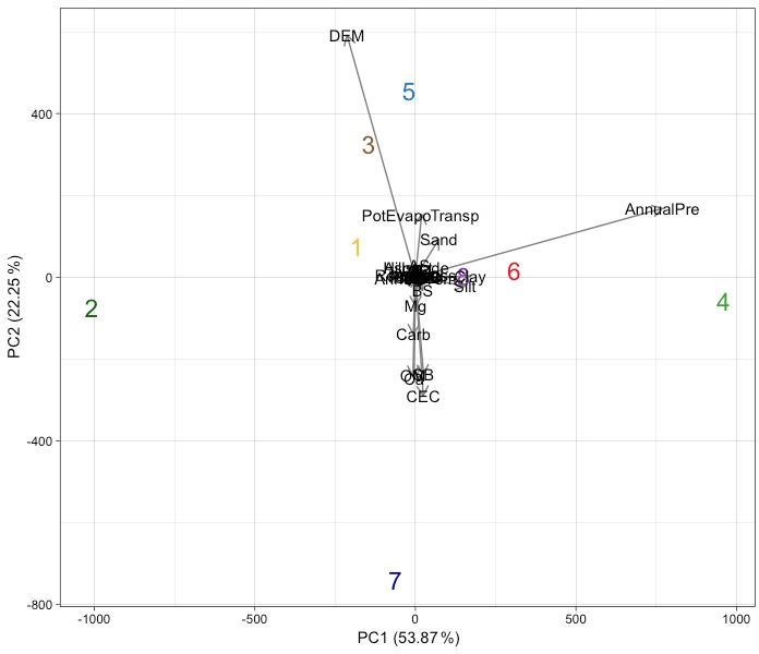
Figure 5 Generalized relationship between the variable and the soil environment grouping (SEG).

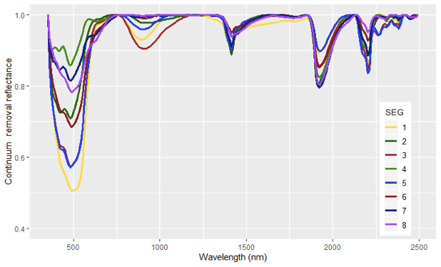
Figure 6 Generalized continuum removal reflectance curve of each soil environment grouping (SEG).

This study sought to develop a quantitative system to group similar soils as an alternative to the traditional taxonomic strategy. The addition of climate and terrain data was beneficial and allowed for SEGs to be better distinguished. Certainly, this is an important indicator of discrepancies in pedologist field observations. In many situations, a same taxonomic soil can be found in very different reliefs. This is a typical situation where soil series would be able to distinguish them, as would SEGs. Moreover, the eight SEGs can be individually categorized by observing their soil, climate, and terrain properties. The generalized relationship between the SEG classes and these properties are shown in Fig. 5. The results show that the proposed classification system could group soils with similar properties. Thus, this study can assist the universal soil system, while demanding less interference from soil analysis, less personal/subjective data, and a higher use of automated devices (such as sensors). Figure 6 shows the shapes of each spectral curve for all of the SEGs.

In summary, we briefly describe the concept and characterization of each SEG.

• SEG 1 refers to soils with a high sand, medium clay, and low silt content; a medium organic carbon content; low fertility; an annual temperature of around 22 ^∘C; a high annual precipitation, soil water balance, and potential evapotranspiration; which are located at a medium elevation.

• SEG 2 refers to soils with a low sand and medium clay and silt content; a medium organic carbon content; low fertility; an annual temperature of around 23 ^∘C; a low annual precipitation and soil water balance, with a medium potential evapotranspiration; which are located at a medium elevation.

• SEG 3 refers to soils with similar sand and clay contents (medium) and a low silt content; a high organic carbon content; medium fertility; an annual temperature of about 20 ^∘C; a high annual precipitation and soil water balance, with a medium potential evapotranspiration; which are located at high elevation (in irregular/roughness areas).

• SEG 4 refers to soils with a low sand content and medium clay and silt contents; a low organic carbon content; high fertility; a high annual temperature of around 26 ^∘C; a high annual precipitation, soil water balance and potential evapotranspiration; which are located at low elevation.

• SEG 5 refers to soils with a high sand content and low clay and silt contents; a low organic carbon content; low fertility; an annual temperature of around 22 ^∘C; high annual precipitation, soil water balance, and potential evapotranspiration; which are located at high elevation.

• SEG 6 refers to soils with a low sand, high clay, and medium silt content; a low organic carbon content; high fertility; an annual temperature of around 21 ^∘C; a high annual precipitation and soil water balance, with a medium potential evapotranspiration; which are located at low elevation.

• SEG 7 refers to soils with a high sand content and low clay and silt contents; a high organic carbon content; high fertility; a high annual temperature of around 23 ^∘C; a medium annual precipitation, high soil water balance, and low potential evapotranspiration; which are located at low altitudes.

• SEG 8 refers to soils with a relatively balanced sand, silt, and clay content, a high organic carbon content; low fertility; a low annual temperature of around 19 ^∘C; a high annual precipitation and soil water balance, with a low potential evapotranspiration; which are located at low elevation.

5 Conclusions

We proposed a quantitative soil grouping system that takes spectral, climate, and terrain variables into consideration. The system was designated as soil environment groupings (SEGs). The system initially indicated a strong relationship with current soil classification (WRB classification system); however, we observed that many different soil classes were inserted into the same group after running the SEG. This occurred because the traditional taxonomic system is sealed and can, therefore, deviate from what is actually observed. The SEG system could define eight groups according to the AIC criteria and clustering analysis. Soil classes such as Ferralsols and Nitisols share many soil and environmental characteristics, which are difficult to distinguish. However, other soil classes, such as Histosols, are relatively distinctive; thus, it was possible to categorize them into a particular SEG. This innovative soil system facilitated the identification and grouping of soils with similar characteristics due to the use of environmental variables. We believe that this classification system can provide the extra information needed for a better understanding of soils in addition to their sustainable management. The development of soil systems such SEG can assist in the distinction of soil types and serve as a new soil data source. The present system follows the pre-existing soil series system which did not gain traction due to several difficulties, including repeatability by different users and its communication between communities. However, owing to the strong computing systems, algorithms, statistical packages, spectral libraries, remote sensing and environmental data (free or open sources) now available, quantitative knowledge has become possible. Therefore, we believe that a soil series system (such as the one proposed here) has the potential to group and discriminate soils.

Appendix A: Supplementary data

Figure A1 Cumulative variance explained for the 10 PCs.

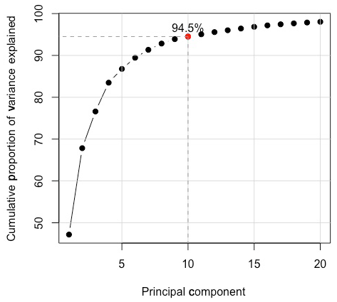
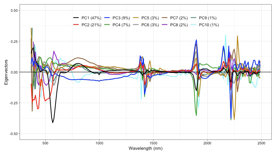
Figure A2 The important spectral features and the contributions of individual wavelengths for PC1–PC10.

Figure A3 The AIC criteria showing that the lowest value was found with eight clusters.

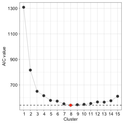
Table A1 Confusion matrix and accuracy of soil classification model (World Reference Base, WRB) using only spectral data.