No silver bullet for digital soil mapping: country-specific soil organic carbon estimates across Latin America

Country-specific soil organic carbon (SOC) estimates are the baseline for the Global SOC Map of the Global Soil Partnership (GSOCmap-GSP). This endeavor is key to explaining the uncertainty of global SOC estimates but requires harmonizing heterogeneous datasets and building country-specific capacities for digital soil mapping (DSM). We identified country-specific predictors for SOC and tested the performance of five predictive algorithms for mapping SOC across Latin America. The algorithms included support vector machines (SVMs), random forest (RF), kernel-weighted nearest neighbors (KK), partial least squares regression (PL), and regression kriging based on stepwise multiple linear models (RK). Country-specific training data and SOC predictors (5 × 5 km pixel resolution) were obtained from ISRIC – World Soil Information. Temperature, soil type, vegetation indices, and topographic constraints were the best predictors for SOC, but country-specific predictors and their respective weights varied across Latin America. We compared a large diversity of country-specific datasets and models, and were able to explain SOC variability in a range between ∼ 1 and ∼ 60 %, with no universal predictive algorithm among countries. A regional (n = 11 268 SOC estimates) ensemble of these five algorithms was able to explain ∼ 39 % of SOC variability from repeated 5-fold cross-validation. We report a combined SOC stock of 77.8 ± 43.6 Pg (uncertainty represented by the full conditional response of independent model residuals) across Latin America. SOC stocks were higher in tropical forests (30 ± 16.5 Pg) and croplands (13 ± 8.1 Pg). Country-specific and regional ensembles revealed spatial discrepancies across geopolitical borders, higher elevations, and coastal plains, but provided similar regional stocks (77.8 ± 42.2 and 76.8 ± 45.1 Pg, respectively). These results are conservative compared to global estimates (e.g., SoilGrids250m 185.8 Pg, the Harmonized World Soil Database 138.4 Pg, or the GSOCmap-GSP 99.7 Pg). Countries with large area (i.e., Brazil, Bolivia, Mexico, Peru) and large spatial SOC heterogeneity had lower SOC stocks per unit area and larger uncertainty in their predictions. We highlight that expert opinion is needed to set boundary prediction limits to avoid unrealistically high modeling estimates. For maximizing explained variance while minimizing prediction bias, the selection of predictive algorithms for SOC mapping should consider density of available data and variability of country-specific environmental gradients. This study highlights the large degree of spatial uncertainty in SOC estimates across Latin America. We provide a framework for improving country-specific mapping efforts and reducing current discrepancy of global, regional, and country-specific SOC estimates.

1 Introduction

Soils store around 1500 Pg of carbon and represent the largest terrestrial carbon pool (Jackson et al., 2017); thus, it is critical to accurately quantify the variability of soil organic carbon (SOC) from local to global scales. During the fourth session of the Global Soil Partnership (GSP) Plenary Assembly held in May 2016 in Rome, it was agreed to develop a Global Soil Organic Carbon Map (GSOCmap) (FAO, 2017). The overarching goal is that a Global SOC Map of the Global Soil Partnership (GSOCmap-GSP) will be developed using a distributed approach relying on country-specific SOC maps. Country-specific maps represent a valuable source of information to explain the high discrepancy of current global SOC estimates such as the SoilGrids250m system and the Harmonized World Soil Database (Tifafi et al., 2018). The Food and Agriculture Organization (FAO) recently compiled how different statistical methods (e.g., regression kriging and machine learning) could be used to generate country-specific SOC maps and calculate uncertainty (Yigini et al., 2018). All these approaches consider the reference framework of the Soils, Climate, Organisms, Parent material, Age and (N) space or spatial position (SCORPAN) model for digital soil mapping (DSM) (McBratney et al., 2003). In the SCORPAN reference framework, a soil attribute (e.g., SOC) can be predicted as a function of the soil-forming environment, in correspondence with soil-forming factors from the Dokuchaev hypothesis and Jenny's soil-forming equation based on climate, organisms, relief, parent material, and elapsed time of soil formation (Florinsky, 2012). The SCORPAN reference framework is an empirical approach that can be expressed as in Eq. (1):

$$\begin{array}{ll}{\displaystyle }{S}_{{\mathrm{a}}_{[x;yt]}}=f& {\displaystyle }(S_{[x;yt]},C_{[x;yt]},O_{[x;yt]},R_{[x;yt]},\\ \text{(1)}& {\displaystyle }& {\displaystyle }{P}_{[x;yt]},A_{[x;yt]}),\end{array}$$

where S_a is the soil attribute of interest at a specific location N (represented by the spatial coordinates of field observations x; y) and at a specific period of time (t); S is the soil or other soil properties that are correlated with the soil attribute of interest (S_a); C is the climate or climatic properties of the environment; O is the organisms, vegetation, fauna, or human activity; R is topography or landscape attributes; P is parent material or lithology; and A is the substrate age or the time factor. To generate predictions of S_a across places where no soil data are available, N should be explicit for the information layers representing the soil-forming factors. These predictions will be representative of a specific period of time (t) when soil available data were collected. Therefore, the prediction factors ideally should represent the conditions of the soil-forming environment for the same period of time (as much as possible) when soil available data were collected. In Eq. (1), the left side is usually represented by the available geospatial soil observational data (e.g., from legacy soil profile collections) and the right side of the equation is represented by the soil prediction factors. These prediction factors are normally derived from four main sources of information: (a) thematic maps (i.e., soil type, rock type, land use type); (b) remote sensing (i.e., active and passive sensors); (c) climate surfaces and meteorological data; and (d) digital terrain analysis or geomorphometry. The SCORPAN reference framework is widely used, but one critical challenge is to quantify the relative importance of the soil-forming factors (i.e., prediction factors) that could explain the underlying soil processes controlling the spatial variability of a specific soil attribute (i.e., SOC).

Arguably, there are two approaches for statistical modeling (Breiman, 2001) that influence the predictions of the spatial variability of SOC. One assumes that the variability of observations can be reproduced by a given stochastic data model (e.g., with hypotheses about the spatial structure of the variable). The other approach uses algorithms and treats as unknown the mechanisms generating the structure of values in available datasets (e.g., with hypothesis about the statistical distribution and moments of the variable). For SOC modeling, the accuracies of global models compared with country-specific estimates have not been systematically evaluated on detail. While globally available SOC predictions rely on large and complex multivariate spaces to represent the soil-forming environment, local (i.e., more simple) models may be useful for validation purposes and required to measure the bias of global SOC estimates, specifically, at particular sites/countries (well represented by available data), where SOC drivers may be easier to identify due to a smaller range of SOC variance. In addition, the assumptions of global models compared with local efforts may be different, and local datasets could complement global information sources. Because different mapping approaches use available information (i.e., training data and predictors) in different ways, comparing several approaches and methods is useful to quantify the relative importance of prediction factors across data configurations and distributional properties. We argue that a systematic analysis of predictive algorithms and consequently selection of predictors (by each one of the algorithms) could provide insights about the underlying factors that control the spatial variability of SOC.

The last decade has seen an increasing diversity of approaches for DSM. Data mining techniques have been successfully used to model and predict the spatial variability of soil properties (Hengl et al., 2017; Rossel and Behrens, 2010; Shangguan et al., 2017) and generate site-specific and country-specific SOC maps (Adhikari et al., 2014; Viscarra Rossel et al., 2014). The combination of regression modeling approaches with geostatistics of independent model residuals (i.e., regression kriging) is a combined strategy that has been widely used to map SOC (Adhikari et al., 2014; Hengl et al., 2004; Kumar et al., 2012; Marchetti et al., 2012; Mishra et al., 2009; Mondal et al., 2017; Nussbaum et al., 2014; Peng et al., 2013; Yigini and Panagos, 2016). Machine learning algorithms such as random forests or support vector machines have also been used to increase statistical accuracy of soil carbon models (Hashimoto et al., 2017; Hengl et al., 2017; Martin et al., 2011) including applications for SOC mapping (Delgado-Baquerizo et al., 2017; Grimm et al., 2008; Hengl et al., 2017; Ließ et al., 2016; Sreenivas et al., 2016; Viscarra Rossel et al., 2014; Yang et al., 2016). Machine learning methods do not necessarily allow to extract information about the main effects of prediction factors in the response variable (e.g., SOC); consequently, a variable selection strategy is always useful to increase the interpretability of machine learning algorithms. With this diversity of approaches, one constant question is if there is a method that systematically improves the prediction capacity of the others aiming to predict SOC across large geographic areas (e.g., Latin America). We postulate that probably there is no universal method (i.e., silver bullet) for DSM, but both global and country-specific efforts are needed to test a variety of predictive algorithms including variable and parameter selection strategies for maximizing explained variance while minimizing prediction bias.

To minimize bias in SOC predictions, it is required to build baseline reference estimates to quantify SOC stocks and contribute to better parameterization for projections of SOC under future soil weathering conditions and land degradation scenarios. Therefore, SOC estimates based on statistical predictions should be ideally based on all available information for specific countries or regions of interest, from both national and global information sources. However, the availability of public SOC information is limited across large areas of Latin America and large discrepancies exist in current global SOC estimates (Tifafi et al., 2018). Thus, there is a pressing need to validate the accuracy of global SOC estimates, improve interoperability (Vargas et al., 2017) and contribute to the capacity of countries to meet the GlobalSoilMap specifications (Arrouays et al., 2017) to inform policy decisions around climate change mitigation strategies.

This study focuses on Latin America, where site- or region-specific modeling efforts report high explained variance when mapping SOC (Reyes-Rojas et al., 2018). Accurate SOC maps are required to identify areas with the potential for soil carbon sequestration, and distinguish them from areas with high SOC. However, site-specific efforts to map SOC across Latin America highlight the challenge of predicting pedologically sound soil maps due to the complexity of SOC spatial variability (Angelini et al., 2016), including the inconsistencies of using simple linear approaches to explain soil and depth interrelationships (Angelini et al., 2017). Site-specific SOC mapping efforts across Latin America also suggest that variable selection and the spatial detail of SOC prediction factors also contribute to discrepancies of SOC predictions (Samuel-Rosa et al., 2015). To increase the accuracy of SOC predictions, the use of high-performance computing through open-source platforms (i.e., Google Earth) represents a valuable resource to make and continuously update (as new and better data become available) country-specific SOC maps (Padarian et al., 2017). The constant challenge is how to increase SOC prediction accuracy while also reducing the uncertainty and granularity of SOC grids.

The overarching goal of this study is to compare different predictive algorithms across 19 data/country scenarios with publicly available information to support the development of country-specific SOC maps to be included in the GSOCmap-GSP. Currently, SOC information across Latin America has been derived from global models such as the SoilGrids system or the Harmonized World Soil Database (Hengl et al., 2017; Köchy et al., 2015), which lack quantification of uncertainty and where large areas remain parameterized with limited country-specific information. This challenge is not unique for Latin America as many regions around the world (e.g., Africa, Siberia) have limited SOC information to parameterize models to estimate the SOC pool. To inform future SOC mapping efforts, this study addresses two specific questions: (a) which environmental variables (derived from publicly available information) have the highest correlations with country-specific SOC information, and (b) which method (i.e., predictive algorithm) is best to represent SOC across Latin America and within each country. We assumed that methods could inform each other as they may explain different aspects of SOC variability. The ultimate aim of this study is to empower capacities for digital SOC mapping across Latin America and to contribute to the discussion about the importance of integrating country-specific information for representing and predicting soil-related variables (e.g., SOC) to improve regional-to-global SOC predictions.

2 Methods

We based our methodological approach on public sources of information and methods implemented in open-source platforms for statistical computing. Thus, our framework for modeling SOC stocks (Fig. 1) could be reproduced across the world for comparative purposes between country-specific and global estimates.

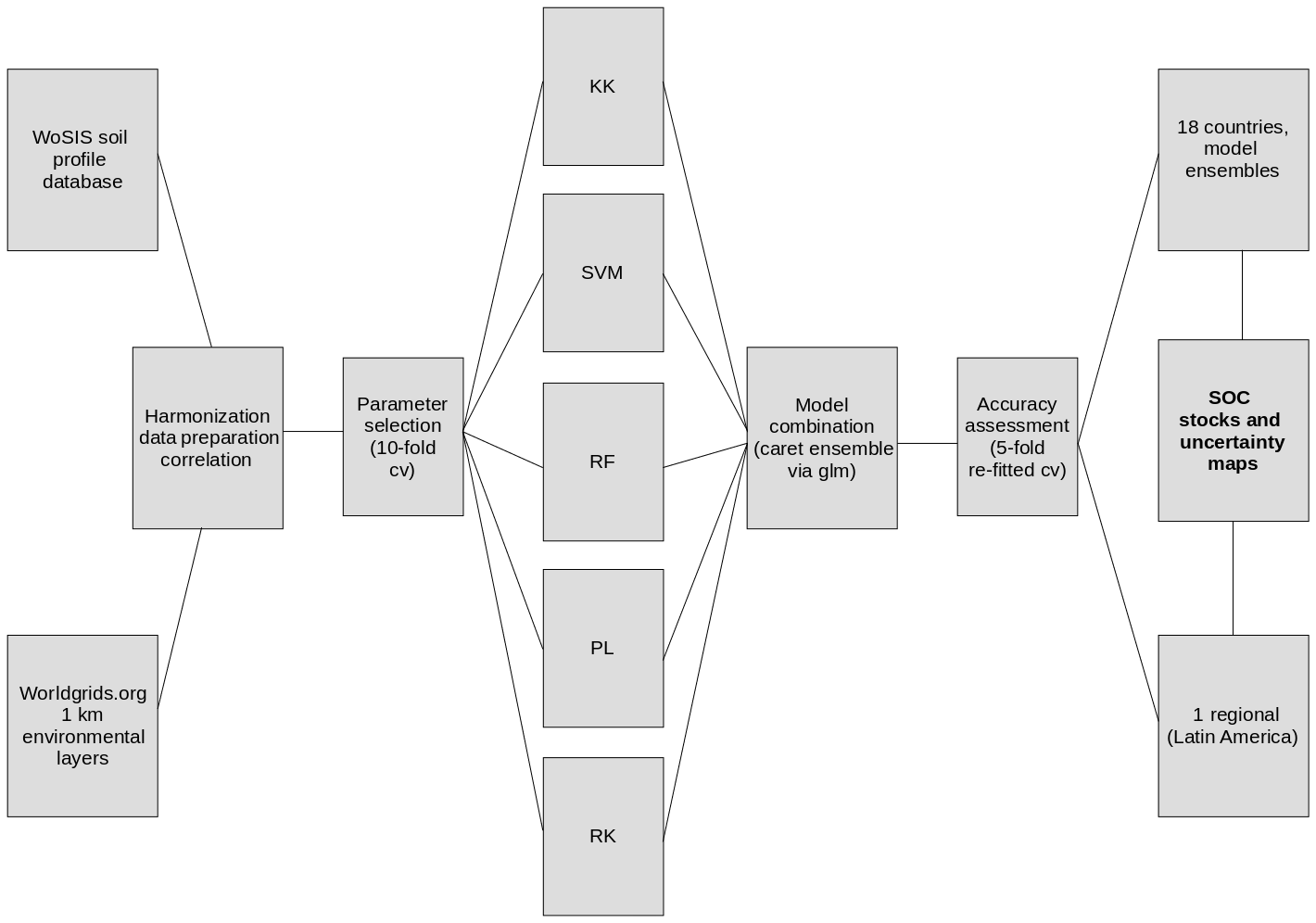
Figure 1 Flow diagram of the main methodological steps that we performed in order to generate country-specific and regional SOC predictions. The World Soil Information Service (WoSIS) dataset was harmonized with the http://worldgrids.org (last access: 20 February 2018) environmental data using 5 × 5 km grids. SOC stocks were calculated at points and correlated predictors identified. Five methods were parameterized and we created an ensemble of using a generalized linear approach. Accuracy of models and the ensembles was assessed with repeated cross-validation. Country-specific and regional (Latin America) ensembles were compared with global models. KK is kernel-weighted nearest neighbors, SVM is support vector machines, RF is random forests, PL is partial least squares regression, and RK is regression kriging.

2.1 SOC observations

Soil organic carbon information was extracted from the World Soil Information Service (WoSIS) soil profile database. This dataset represents a great harmonization effort in which a large number of national legacy datasets have been compiled. It includes local-to-national soil profile collections with a sampling strategy generally based on morphological soil attributes (Batjes et al., 2017). The goal of the GSOCmap-GSP is to produce global information for the first 30 cm; thus, we generated synthetic horizons for this depth using a mass-preserving spline approach (Bishop et al., 1999). We applied a pedotransfer function based on organic matter (OM) if the bulk density (BLD) information was missing: BLD is $\mathrm{1}/(\mathrm{0.6268}+\mathrm{0.0361}\times \mathrm{OM})$ (Yigini et al., 2018). We decided to use this equation because it showed less extreme values than other available pedotransfer functions during preliminary discussion and training exercises (data not shown). Another reason is that there is not a single pedotransfer function applicable to all conditions across Latin America. This equation is representative for soils with organic matter content between 0.17 and 13.5 % (Drew, 1973). For coarse fragments (CRFVOL), a value of 0 % was used for missing information prior to the mass-preservative spline modeling. SOC estimates (0 to 30 cm) were derived following a standardized SOC calculation method (Nelson and Sommers, 1982) (Eq. 2):

$$\begin{array}{}\text{(2)}& {\mathrm{SOC}}_{\mathrm{stock}}={\displaystyle \frac{\mathrm{ORCDR}}{\mathrm{1000}}}\times {\displaystyle \frac{H}{\mathrm{100}}}\times \mathrm{BLD}\times {\displaystyle \frac{(\mathrm{100}-\mathrm{CRFVOL})}{\mathrm{100}}},\end{array}$$

where ORCDR is SOC density (g kg⁻¹) and H is soil depth (30 cm).

Because of the limitations and uncertainty in the available BD and CRFVOL data, we also included an error approximation of SOC estimates. This error was derived using Global Soil Information Facilities (GSIF; Hengl, 2017) as explained in the next section.

2.2 SOC error estimates

The GSIF approach for estimating SOC (function OCSKGM) includes an approximate error which we used to quantify the reliability of SOC estimates (Hengl et al., 2017). This error was approximated using the Taylor series method, by a truncated Taylor series centered by the means explained previously (Heuvelink, 2018). We mapped the error trend of SOC estimates by interpolating the values on a per country basis using the generic framework for predictive modeling based on machine learning and buffer (geographical) distances (Hengl et al., 2018). We followed this method to provide a spatial explicit measure of the SOC estimation error. We used this method because it can be implemented without prediction factors (e.g., only buffer distances) and because it is practically free of assumptions but considers the geographical proximity to and composition of the sampling location points as explained by its developers (Hengl et al., 2018). SOC error estimates represent a component of uncertainty of the overall quality of country-specific input data.

2.3 SOC training data and exploratory analysis

Each country-specific SOC dataset was transformed to its natural logarithm to reduce the right-skewed distribution of SOC values and because exploratory analysis showed that this transformation can improve the prediction capacity of further modeling methods. To analyze the statistical distribution of SOC values, a probability distribution function was plotted and a Shapiro–Wilk test of normality was conducted on each dataset. The units of the SOC estimates are kg m⁻². Our global (Latin America) dataset of 11 268 SOC estimates was divided using a simple bootstrapping technique (Kuhn et al., 2017) and 25 % of data were used for independent validation purposes, and the remaining 75 % of data for training prediction models. We coupled this information with a public source of prediction factors; see Sect. 2.4.

2.4 Soils prediction factors

We used environmental information from WorldGrids (worldgrids.org), which is an initiative of ISRIC-World Soil Information. We downloaded and masked 118 environmental layers (i.e., prediction factors) for each country to quantitatively represent the soil-forming environment (http://worldgrids.org/doku.php/wiki:layers, last access: 20 February 2018). The prediction factors were harmonized into a 1 × 1 km global grid by the WorldGrids project from three main information sources: remote sensing, climate surfaces, and digital terrain analysis. Additional terrain parameters (e.g., terrain slope, aspect, catchment area, channel network base level, terrain curvature, topographic wetness index, and length–slope factor) from elevation data were calculated in the System for Automated Geoscientific Analyses geographic information system (SAGA GIS) for each country following the standard implementation for basic terrain parameters (Conrad et al., 2015). We resampled the prediction factors into a 5 × 5 km pixel size grid to reduce the computational demand required to make predictions and facilitate the reproducibility of this DSM framework without the need for high-performance computing.

2.5 Prediction of SOC

We made predictions on a country-specific and on a regional (Latin American) basis. We based our prediction framework on the following six steps:

• First, the relationship between SOC and prediction factors was explored using simple correlation analysis.

• Second, the 10 prediction factors with highest correlations with SOC data were identified for each country and used for further analyses.

• Third, we explored, parameterized, and compared five statistical methods with different assumptions to model SOC variability across Latin America: regression kriging (based on a multiple linear regression model (RK) and partial least squares (PLS) regression, support vector machines (SVMs), random forests (RF), and kernel-weighted nearest neighbors (KK). A brief explanation for each modeling approach is provided in Appendix A.

• Fourth, we used a five times repeated 5-fold cross-validation strategy of the aforementioned models to estimate the RMSE. Then, we used the caretEnsemble tools for stacking the five predictions (Deane-Mayer and Knowles, 2016; Kuhn et al., 2017). The caretEnsemble approach uses the RMSE to weight and create ensembles of regression models under a generalized approach to create a linear blend of predictions.

• Fifth, we calculated independent model residuals (by predicting the 25 % of data not used for model parameterization). For each 5 × 5 km pixel, we estimated the full conditional response of these residuals to the SOC prediction factors following the quantile regression method available within the quantregForest modeling framework (Meinshausen, 2006, 2017). We used this map as a surrogate of model uncertainty complementary to the approximated error trend of SOC estimates.

• Sixth, we used all Latin American data in the WoSIS system to repeat the fourth and fifth steps of our modeling framework, generating regional predictions of SOC and comparing with country-specific results and global SOC estimates. We also evaluated the prediction capacity of these models.

2.6 Model evaluation and accuracy

First, we selected the optimal parameters for each model/country by the means of a 10-fold cross-validation strategy following a generic recommendation (Borra and Di Ciaccio, 2010) (see parameter description in Appendix A). For each model, the train function of the caret package (Kuhn et al., 2017) included simple resampling techniques for automatic model parameter selection. Thus, we obtained unbiased residuals for each model/country that we compared using Taylor diagrams (Carslaw and Ropkins, 2012). A Taylor diagram summarizes multiple aspects of model performance, such as the agreement and variance between observed and predicted values (Taylor, 2001). In a Taylor diagram, each model is represented by a point in the plot describing how well the patterns of observed and modeled values match each other. Two models have a similar predictive capacity if they overlap across the intersection of an error vector, a variance ratio, and a correlation vector.

We analyzed the overall ratio (EC_r) between model errors (RMSE) and the correlation between observed and predicted values (corr) for each model across all countries. We propose this ratio EC_r as an approach to better understand the agreement between the correlation (calculated by the means of cross-validation) and the RMSE (derived from the unbiased residuals of cross-validation). Before calculating the RMSE ∕ correlation ratio, the RMSE and the correlation between observed and predicted values were standardized (by its maximum and minimum values) to a range between 0 and 1 using

$$\begin{array}{}\text{(3)}& {\displaystyle }& {\displaystyle }{\text{RMSE}}_{\mathrm{SD}}={\displaystyle \frac{{\text{RMSE}}_i-min\left(\text{RMSE}\right)}{\mathrm{range}\left(\text{RMSE}\right)}}\text{(4)}& {\displaystyle }& {\displaystyle }{\text{corr}}_{\mathrm{SD}}={\displaystyle \frac{{\text{corr}}_i-min\left(\text{corr}\right)}{\mathrm{range}\left(\text{corr}\right)}}\text{(5)}& {\displaystyle }& {\displaystyle }{\mathrm{EC}}_{\mathrm{r}}={\displaystyle \frac{{\text{RMSE}}_{\mathrm{SD}}}{{\text{corr}}_{\mathrm{SD}}}},\end{array}$$

where EC_r is the proposed ratio between errors and correlation between observed and predicted values; RMSE_i is the observed RMSE for the ith model; min(RMSE) is the minimum observed value of RMSE, and range(RMSE) is the difference between the maximum and minimum observed values of RMSE; corr_i is the observed correlation for the ith model; min(corr) is the minimum observed value of correlation, and range(corr) is the difference between the maximum and minimum observed values of correlation

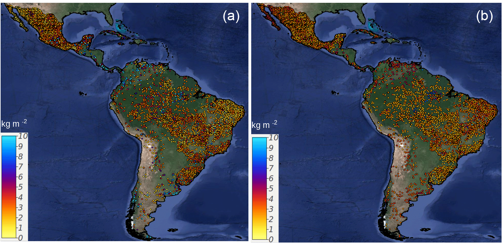
Figure 2 Spatial distribution of available SOC in WoSIS for Latin America. SOC estimates are calculated for each point using Eq. (2) (a). The approximated error is based on Taylor series as implemented in the R-GSIF package, as is explained in Heuvelink (2018) (b). Thus, panel (b) represents the uncertainty of SOC estimates at each point. The values of this map could be associated with data limitations and missing information for BLD and CRFVOL.

If the value of the EC_r was close to 0, then there was a stronger agreement between high RMSE and low correlation, or low RMSE and high correlation. If this value deviated from 0 (up to 1 or more), then the RMSE would tend to be high while the correlation was also high, suggesting that the method represented the variability of SOC but with high bias.

Model accuracy (also represented by the RMSE and R²) was assessed for the model ensembles with a more strict (but computationally expensive) 5-fold and five times repeated cross-validation strategy. This model refitting allowed more stable accuracy results with the ultimate goal of comparing country-specific and regional (Latin America) estimates. Repeated 10- and 5-fold cross-validation have been used to compare both machine learning and geostatistical approaches for mapping soil properties from book examples to real applications at the global scale (Hengl et al., 2017, 2018). In addition, independent model residuals were also obtained from the 25 % of data not used for the country-specific and regional ensembles to estimate a spatially explicit measure of uncertainty (as explained in step five of our prediction framework).

2.7 SOC stocks

First, we analyzed the influence of the maximum allowed prediction limits for each prediction algorithm. We harmonized the units of our SOC estimates with global datasets in Mg ha (megagrams per hectare at 30 cm depth). The sensitivity of the total SOC stock to the model prediction limit was tested by increasing (every 10 Mg ha) the maximum prediction limit from 0.5 Mg ha. until finding a stable rate. Geopolitical limits were obtained from the Global Administrative areas project (https://gadm.org/, last access: 16 July 2018). Using these country limits we report our country-specific and Latin American SOC estimates. For comparative purposes, we also extracted for each country the global SOC estimates from the SoilGrids system (Hengl et al., 2017), the Harmonized World Soil Database (Köchy et al., 2015), and the GSOCmap-GSP (see http://54.229.242.119/apps/GSOCmap.html, last access: 16 July 2018). We also report stocks across the land cover classes derived from the Latin American Network for Monitoring and Studying of Natural Resources, a product with an estimated accuracy of 84 % (Blanco et al., 2013). We report the overall uncertainty of these stocks with the independent model residuals map and the approximated error trend of the SOC estimates. Some countries with no data were filled with the average of the surrounding extent of the SOC predictions. All analyses were performed using the R software (R Core Team, 2017).

3 Results

3.1 Descriptive statistics

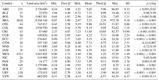
SOC across different countries showed a wide diversity of data scenarios (Table 1). Costa Rica (with a mean of 11.05 kg m²), Chile (with a mean of 9.88 kg m²), and Colombia (with a mean of 8.15 kg m²) are the countries with the highest SOC mean values. Brazil (n=5616) and Mexico (n=4321) were the countries with highest data availability. In contrast, Honduras (n=11), Guatemala (n=20), and Belize (n=21) were the countries with lowest density of SOC estimated values (Table 1). With the original (untransformed) dataset, the only countries that showed a normal distribution after the Shapiro–Wilk test of normality with an α of 0.05 were Belize, Guatemala, Honduras, and Suriname.

Table 1 Descriptive statistics of SOC estimates (in kg m²) and total land area for each analyzed country. n is the number of observations. We provide quantiles, median, mean, and the standard deviation of SOC data. The columns p and plog represent the probability values derived from the Shapiro–Wilk test of normality before p and after plog the log transformation of SOC values. When p is larger than plog, the log transformation of the data did not increase the probability of normality in the dataset. For comparative purposes, we provide (Fig. S1 in the Supplement) the probability distribution functions of available data before and after the log transformations. ARG is Argentina, BLZ is Belize, BOL is Bolivia, BRA is Brazil, CHL is Chile, COL is Colombia, CRI is Costa Rica, CUB is Cuba, ECU is Ecuador, GTM is Guatemala, HND is Honduras, JAM is Jamaica, MEX is Mexico, NIC is Nicaragua, PAN is Panama, PER is Peru, SUR is Suriname, SLV is El Salvador, URY is Uruguay, and VEN is Venezuela.

3.2 Spatial distribution and point error estimates

There were large areas of Latin America with no available SOC observational data in the WoSIS system (e.g., the south of Chile, Argentina, or across large areas of Central America). We found substantial error estimates across large areas with high density of SOC data but low carbon contents, such as northern Mexico or the Brazilian semiarid savanna located at the eastern side of that country (Fig. 2).

3.3 Correlation of SOC and its predictors

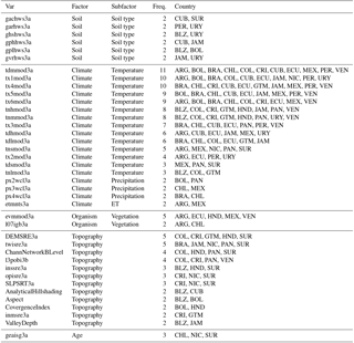
Best correlated predictors were not the same across countries. We found higher correlations with the original datasets transformed to their natural logarithm, as data had a right-skewed distribution and did not follow a normal distribution (i.e., log normal). Highest correlations of available SOC data and their environmental predictors were associated with temperature-related variables across Honduras, Costa Rica, Peru, Chile, Guatemala, and Suriname (the r² varied from 0.35 to 0.58). However, there were a low number of available SOC observations across these countries in the WoSIS system (between 11 to 34). Similarly, across countries with high data availability (e.g., Mexico and Brazil), the strongest correlations between SOC and prediction factors were associated with temperature-related variables (Table 2). In all cases, the relationship between SOC and temperature-related variables was negative. In contrast, SOC had a positive relationship with elevation-derived terrain parameters (r² varied from 0.43 to 0.59) such as terrain curvature, potential incoming solar radiation, and slope of terrain.

Lower correlations of SOC data with prediction factors were found across Brazil, Bolivia, Uruguay, Cuba, Panama, Venezuela, and Argentina (e.g., r² < 0.2). The correlation analysis was useful to formulate a working hypothesis about the major drivers of the spatial variability of SOC across countries based on our DSM conceptual framework (e.g., SOC_ARG = f[px4wcl3a + px3wcl3a + evmmod3a + l07igb3a + px2wcl3a + …]). For example, the best correlated predictors with SOC for Argentina were precipitation-related variables (px4wcl3a, px3wcl3a, px2wcl3a), remote-sensing-based vegetation indexes (evmmod3a), and a probability-based shrubland map (l07igb3a) (Table 2) (see sources of these maps in http://worldgrids.org/doku.php/wiki:layers, last access: 20 February 2018).

Table 2 Best correlated predictors and their frequency across the analyzed data country scenarios, given available data in the WoSIS system; see predictor codes in http://worldgrids.org/doku.php/wiki:layers (last access: 20 February 2018). ARG is Argentina, BLZ is Belize, BOL is Bolivia, BRA is Brazil, CHL is Chile, COL is Colombia, CRI is Costa Rica, CUB is Cuba, DOM is Dominican Republic, ECU is Ecuador, GTM is Guatemala, HND is Honduras, JAM is Jamaica, MEX is Mexico, NIC is Nicaragua, PAN is Panama, PER is Peru, SUR is Suriname, SLV is El Salvador, URY is Uruguay, and VEN is Venezuela.

3.4 SOC-related properties

Correlations between SOC density (ORCDR) and prediction factors were higher with maximum and mean nighttime temperature, where Costa Rica and Chile had the highest correlations (r² varied from 0.61 to 0.71). The best correlated variables with BLD were terrain parameters: relative slope position, vertical distance to channel network, flow accumulation areas, and potential incoming solar radiation. These correlations were stronger across Guatemala, Belize, and Panama (r² varied from 0.52 to 0.67). We found that terrain slope and the standard deviation of temperature were the variables with highest correlations with CRFVOL, where Nicaragua, Honduras, and Argentina had the highest correlations (r² varied from 0.40 to 0.55). We did not find a dominant algorithm to predict ORCDR, BLD, and CRFVOL. Slightly higher correlations between observed and predicted values were achieved with RF, but in most cases different methods showed similar prediction capacity. The highest prediction error was found with RK for CRFVOL, but for all other output variables all prediction algorithms had a similar range of errors (Fig. 3). The PLS and SVM had the lowest variance for prediction of each one of the four soil properties. The r² values for predicting the combined SOC-related properties (i.e., ORCDR, CRFVOL, and BLD) for each prediction algorithm were RK (r² 0.67 to 0.76), RF (r² 0.56 to 0.74), SVM (r² 0.32 to 0.71), PL (r² 0.46 to 0.69), and KK (r² 0.19 to 0.64). Across countries with lower data availability and sparse distribution, SVM and RK algorithms resulted in lower model performance.

Figure 3 Taylor diagrams showing the performance of the five models evaluated. SOC stock (a), ORCDR (b), BLD (c), and CRFVOL (d). This analysis is based on all available data across Latin America. Although RF tends to generate higher correlation, it also shows high variance in predictions. The points are close to each other and the differences in accuracy between them generally fall within the same intersection of error, variance, and correlation, suggesting a similar prediction capacity by the implemented approaches.

3.5 Country-specific SOC predictions

We did not find a dominant algorithm to predict SOC on a country-specific basis (Fig. 4). Overall, machine learning prediction algorithms generated similar results. Higher agreement of machine learning prediction algorithms was found in small countries where environmental conditions and land cover/use characteristics tend to be more homogeneous (e.g., Jamaica, Suriname). RK showed higher discrepancies in countries where data distribution was sparse (e.g., Suriname, Chile, Guatemala) but effective across countries with higher and/or well-distributed data availability (e.g., Mexico, Brazil). Machine learning SOC predictions were conservative compared with RK (RK generated the higher density of extreme and unreliable SOC values). PL had comparable results with machine learning algorithms (i.e., KK, SVM, RF). From the cross-validation strategy, higher r² values between observed and predicted data were found for Costa Rica (0.58; n=21) using SVM, while the lowest error was found in Suriname (0.36 kg m⁻²; n=37) using PL. In contrast, algorithms had lower prediction capacity for countries with large areas (e.g., Brazil, Mexico) despite the large data availability.

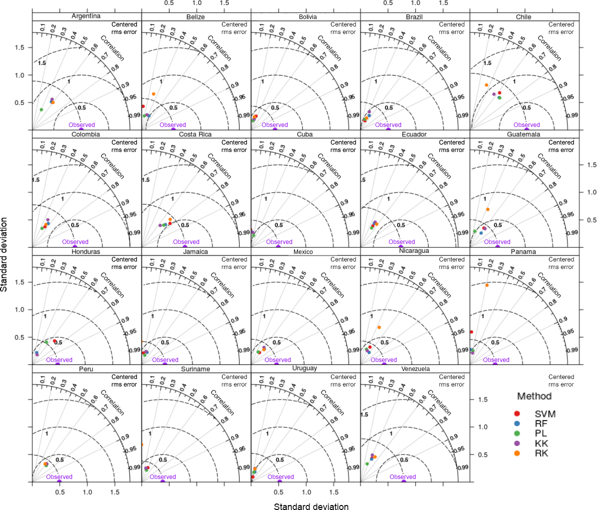
Figure 4 Taylor diagrams showing the performance of the five models evaluated for country-specific SOC estimates across Latin America. The position of each point/method varies from each dataset to another, suggesting that the predictive capacity changes when data characteristics are different.

The simple correlation (main effect) between the r² and RMSE for RF, PL, KK, and RK was positive (0.18, 0.35, 0.32, and 0.1, respectively). In contrast, this correlation was stronger for SVM (but negative; −0.65) where increasing the explained variance resulted in a lower error. Thus, we found a low level of agreement between these two information criteria (r² and RMSE) commonly used in DSM to assess performance of prediction algorithms.

Agreement between the RMSE and r² was found only in 12 of the 19 countries, resulting in country-specific “recommended” prediction algorithms. Here, we list the prediction algorithms that generated the best correlation and the best RMSE for each country: ARG (RK, RK), BLZ (RF, RK), BOL (SVM, KK), BRA (RF, RF), CHL (PL, PL), COL (RF, RF), CRI (SVM, SVM), CUB (PL, PL), ECU (RK, RK), GTM (KK, RF), HND (SVM, KK), JAM (RF, RF), MEX (RK , RK), NIC (RF, RF), PAN (PL, KK), PER (KK, KK), SUR (SVM, PL), URY (RF, RK), and VEN (RK, RK) (see country codes in Table 1). Brazil and Mexico had the highest number of observations (nearly 80 % of the total) and the same method yielded the highest r² and the lowest RMSE. We clarify that the best within-country method was not the same for every country. The higher EC_r was found with PL (0.96), followed by RF (0.54) and KK (0.43), informing that these predictive algorithms did not minimize prediction bias while increasing the explained variance. SVM (with 0.008) and RK (with 0.003) had the lowest EC_r, as they maximize the explained variance while minimizing prediction bias.

3.6 Model ensembles and SOC maps

High discrepancy was found among country-specific SOC predictions and between country-specific and regional SOC predictions. Although both maps predict SOC following a similar general pattern, the country-specific ensemble showed a higher density of unrealistic patterns across Guatemala, Venezuela, northern Brazil, and the surroundings of Uruguay (Fig. 5a). These areas correspond to areas where we report both higher SOC calculation errors and model uncertainty (Fig. 6).

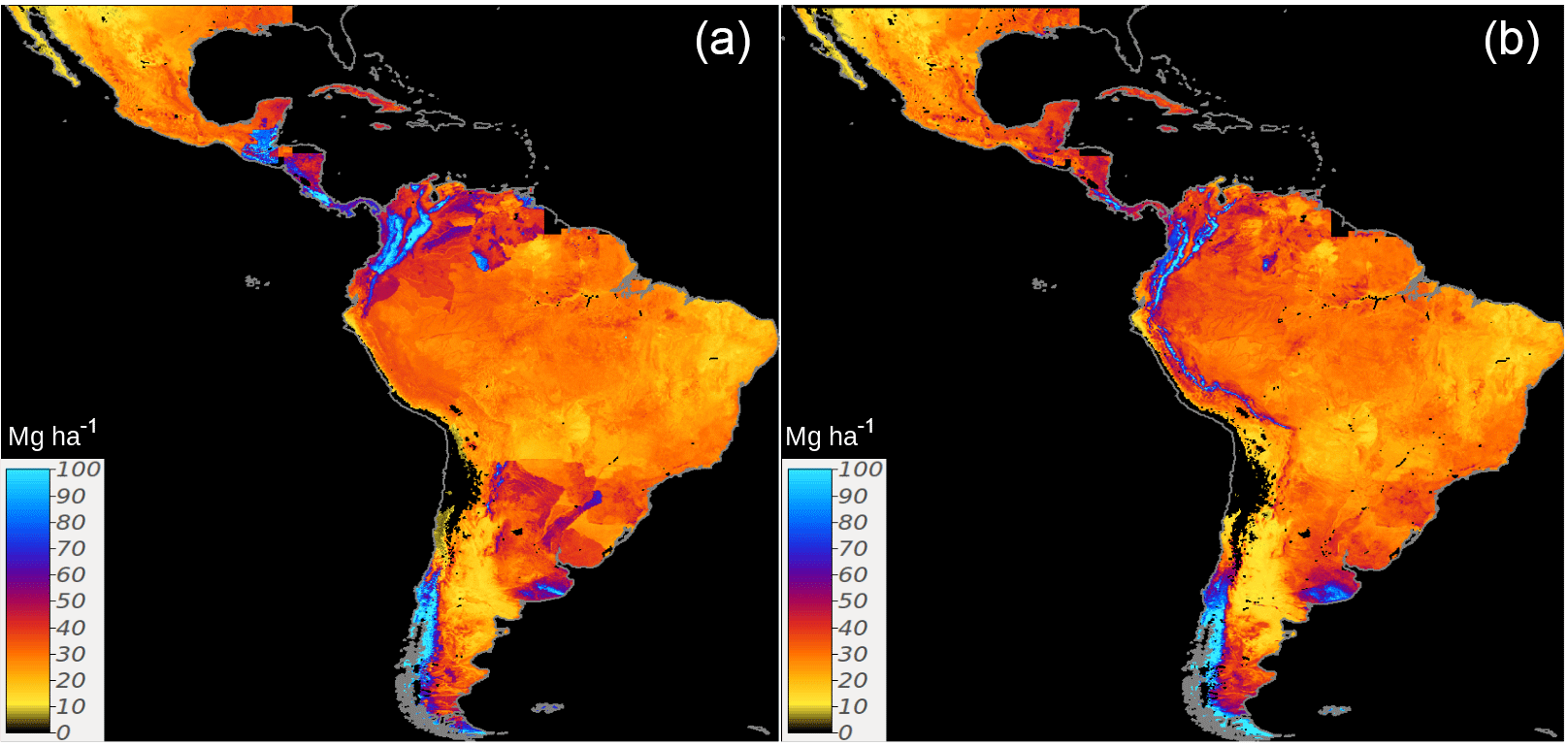
Figure 5 Country-specific (a) and regional (Latin America) (b) predictions of SOC based on a linear ensemble of methods. We present the units as Mg ha for visualization purposes. These units were used to reduce the digits of the value range and highlight larger differences between SOC maps.

Compared with the country-specific ensemble, the regional model showed spatial differences predicting higher SOC across the highlands of the Southern Andes and boundaries of the Amazon Basin (Fig. 5b). As expected, the country-specific model showed spatial artifacts associated with country geopolitical borders. Based on the repeated 5-fold cross-validation, we report a r²=0.39 for the regional model and r² values for the country-specific approach that vary from 0.01 to 0.55.

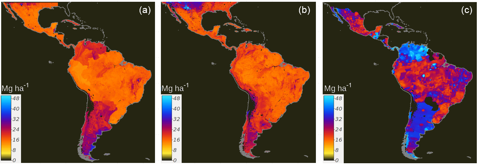
Figure 6 The full conditional response of residuals to the prediction factors on a country-specific basis (a). The full conditional response of residuals to the SOC prediction factors in the regional (Latin America) model (b). The trend of the approximated error of SOC estimates is derived from buffer distances and the random forest spatial framework (c).

High uncertainty in our modeling framework was found across tropical, arid, and semiarid regions of Latin America (Fig. 6a, b). Residual uncertainty from independent validation in the country-specific ensemble showed higher errors across geopolitical borders (in Chile, Argentina, Colombia, Ecuador, Venezuela, and the Brazilian savanna), while the residual uncertainty map from the regional model had higher uncertainty across ecologically meaningful transitions, with no evident effect of geopolitical borders. The trend of the mean approximated error suggests high uncertainty in the SOC calculation method (Fig. 6c). We used this map just to visualize the general trend of error estimates based only on geographical buffer distances.

Primarily, the Pacific coastal plains, the delta of the Amazon river, some closed watersheds and wetlands across Mexico, and some sparse points across Central America showed the higher discrepancies. Mexico and Brazil, with higher density of SOC data, were the countries with less discrepancy between country and global models (Fig. 7a). We report that the geographical areas where country-specific models tend to predict higher SOC values than the regional ensemble (Fig. 7b). However, we report a similar SOC stock from both modeling approaches (country-specific and global) as we explain in Sect. 3.7.

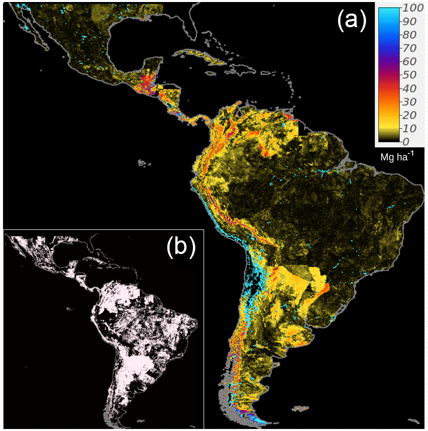
Figure 7 The absolute distance (Mg ha) between the country-specific and the regional ensemble (a). The areas in white are areas where the country-specific modeling is predicting higher SOC than the regional estimate (i.e., country-specific is greater than regional) (b).

3.7 SOC stocks and model uncertainties

For comparative purposes with previous reports (i.e., the SoilGrids system and the Harmonized World Soil Database), we harmonized the units of our maps to Mg ha, which was also useful for visualization purposes. For our models, the uncertainty of the maximum prediction limit was estimated to be ±10 Pg, which was the variance of the SOC stock by increasing the prediction limit from 1 to 700 Mg ha (Fig. 8). This relationship showed a stable (close to 0) trend after 200 Mg ha. A larger density of extreme values was found with the regional model, and we calculated a maximum possible SOC stock of 83.62 Pg with this model.

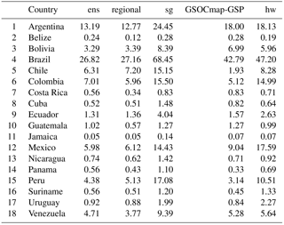
Despite the spatial differences reported for the country-specific and regional ensembles, we report a similar stock between both approaches (77.8 ± 42.2 and 76.8 ± 45.1 Pg, respectively). We found that the global ensemble yields a slightly higher uncertainty. Our country-specific ensembles suggested that countries with highest SOC stocks were Brazil, Argentina, Colombia, Mexico, Peru, and Venezuela (Table 3).

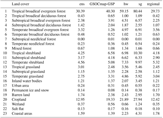
Consistently, all models showed that tropical broadleaf evergreen forests, croplands, and temperate shrublands were the land cover classes that had higher SOC across all SOC available estimates (Table 4). However, using only the dataset contained in the WoSIS system, we predict nearly the half of SOC compared with previously reported SOC estimates such as the SoilGrids system (Table 3).

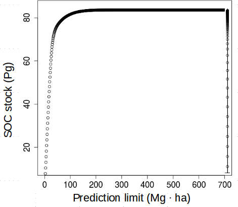
Figure 8 Relationship between the SOC stock and the prediction limit. The average breakdown points of this relationship are shown in the vertical line at the right of the plot.

Table 3 SOC stocks (Pg) at the contextual resolution of 5 × 5 km grids. The terms used are defined as follows: ens is country-specific, regional is Latin America ensemble, sg is the SoilGrids system, GSOCmap-GSP is country-specific 1 km, and hw is the Harmonized World Soil Database.

The model variance of predicted SOC reached values over 300 % for countries such as Mexico and Bolivia. In contrast, countries with higher SOC per unit area and relatively low prediction variances were Panama, Guatemala, Costa Rica, Nicaragua, and Belize. Overall, we found a median model prediction variance of 53 % across countries in Latin America. Areas with high uncertainty and model variance were across northern Mexico, Central America, limits between Colombia and Brazil, and the border between Chile and Argentina.

4 Discussion

We developed a DSM framework to characterize the spatial variability of SOC across Latin America. Our results suggest that a multi-model approach was suitable to better understand modeling bias and uncertainty of SOC maps. We argue that uncertainty on SOC mapping can be associated with (a) the complexity of the property of interest (i.e., SOC), (b) the environmental heterogeneity within the area/country of interest, and (c) the characteristics of available data (e.g., data density, data quality, and data representativeness) to meet model-specific assumptions. Thus, when legacy soil profile collections that were collected for different purposes along long periods of time (i.e., decades), a multi-model approach (i.e., ensemble) would be convenient to maximize the predictive capacity considering the available information.

To maximize accuracy of our models, we used a generalized linear approach to combine single predictions, and at the continental scale we were able to explain 39 % of SOC variance using only information contained in the WoSIS system for Latin America. This result was within the range of the prediction capacity of country-specific models. Besides the low density of observation points, the performance could be partially affected by the generalization from the 1 : 1 scale of a soil profile (or field SOC observation) to a 5 × 5 km grid, representing an additional source of uncertainty. Higher discrepancy between country-specific and global efforts was evident across Brazil, the largest country, where our models tend to predict nearly half of SOC compared to previous efforts (e.g., the GSOCmap-GSP, the SoilGrids system, and the Harmonized World Soil Database). The SoilGrids system tends to predict the highest values, while our country-specific ensemble predicts the lowest. The GSOCmap-GSP and our ensembles predicted < 100 Pg of SOC across the analyzed countries, while all other products suggest higher stocks (see Tables 3 and 4).

Another source of discrepancy can be associated with the lack of available data to represent the SOC stock at the depth of interest (i.e., −30 cm of mineral soil). The predictive performance of the mass-preservative spline to continuously represent the SOC and depth relationships in some cases could be strongly influenced by the lack of observations across highly variable soil profiles. Some examples include SOC-rich agricultural soil profiles constantly transformed for food production purposes, or a volcanic setting. These high levels of missing data lead the trend map of approximated error (Fig. 6), which provides an idea of the uncertainty in the SOC estimates.

Table 4 SOC stocks at the contextual resolution of 5 × 5 km across land cover classes of Latin America for the 18 analyzed countries. The terms used are defined as follows: ens is country-specific, regional is Latin America ensemble, sg is the SoilGrids system, GSOCmap-GSP is country-specific 1 km, and hw is the Harmonized World Soil Database. These are the land cover classes described in Blanco et al. (2013). This land cover product was generated using 500 m grids and has 84 % of accuracy.

The GSOCmap-GSP, for example, was generated on a country basis, but the amount of SOC observations used for the countries to generate these maps was considerable higher than the available data in the WoSIS system (> 1 000 000 points). Both of our models predicted more conservative results than the GSOCmap-GSP, while at the same time, the GSOCmap-GSP predicted less SOC than the SoilGrids system and the Harmonized World Soil Database. Respectively, the SoilGrids system relies on a multivariate space suitable to represent the global soil-forming environment; however, a model would assume a similar relation of each covariate with the response across all land area in the world. The Harmonized World Soil Database may be a pedologically sound product, but large areas of Latin America have not been mapped at detailed scales (i.e., larger scales than 1 : 1 million) and this results in a polygon-based approach relying on wide generalizations.

Despite the aforementioned limitations, across Latin America, there is an increasing availability of relevant SOC information across site- and country-specific regions (Angelini et al., 2016, 2017; Padarian et al., 2017; Reyes-Rojas et al., 2018; Samuel-Rosa et al., 2015; Vasques et al., 2016), which could serve for validating and calibrating global SOC estimates. Thus, regional approaches considering multiple Latin American countries and SOC models could be a valuable resource to explain discrepancies between site- or country-specific and global SOC models.

Our results incorporate a multi-model perspective for quantifying/evaluating the spatial variability of SOC. The model with higher predictive capacity in terms of cross-validated r² was RF, an ensemble of regression trees based on bagging. However, this method yields high EC_r, and therefore it tends to capture the trend but with high bias. Taylor diagrams show that RF in any case yield the lower variance. SVM and RK were methods with higher agreement between RMSE and corr, and therefore lower EC_r. Large values of EC_r represent an accuracy limitation that was evident for RF, PL, and KK. To overcome these types of modeling biases, previous studies have suggested that the theory of ensemble learning applied to soil datasets could increase the accuracy of results (Finke, 2012; Nussbaum et al., 2018). Furthermore, recent studies highlight the applicability of selective ensembles across a large diversity of model algorithms useful for digital soil mapping purposes (Møller et al., 2018). Thus, our modeling approach included the combination of multiple predictions by using a linear stack of models as implemented in the caretEnsemble package of R (Deane-Mayer and Knowles, 2016), with the ultimate goal of reducing the uncertainty on SOC mapping efforts.

Across Latin America, we did not find a common predictive algorithm for SOC. These results suggest that country-specific environmental predictors and available data influence the applicability of different approaches. This assessment is needed to address the requirements from the GSOCmap-GSP with the official mandate to generate and update country-specific soil information by the means of DSM. Thus, we argue that the DSM form of each country should assess and incorporate country-specific available data and environmental predictors to select the best prediction algorithm. The FAO SOC mapping cookbook explores possibilities to derive country-specific SOC maps from a variety of prediction algorithms (Yigini et al., 2018), and multiple resources have described the state of the art of modeling methods focused on DSM of soil carbon (Malone et al., 2017; Minasny et al., 2013) including geostatistics (Hengl, 2009, 2017). Thus, data characteristics (e.g., spatial structure, representativeness) are specifically important for developing a DSM framework as legacy soil profile collections, generated with long-term soil inventory purposes, will determine data availability and spatial distribution within a country.

This country-specific approach to map regional SOC results in artifacts across geopolitical borders. Therefore, data sharing, model validation, and calibration experiments among countries are required to better capture the spatial variability of SOC. The use of a natural-defined prediction domain (e.g., ecoregional or physiographic map) could reduce the border effects. However, we understand that geopolitical borders are required for policy decisions around country-specific needs. We highlight that there is a lack of publicly available country-specific data that ultimately influence the performance of both country-specific to regional-to-global SOC estimates.

To achieve the highest possible accuracy of country-specific SOC estimates, the availability of point data sources for SOC modeling and mapping is an important consideration when selecting an efficient modeling strategy, especially when dealing with legacy SOC datasets. Our results highlight important uncertainty levels (> 100 %) across large areas of Latin America (Table 6). The data contained in WoSIS have a low-density distribution given the large area and environmental complexity of several countries analyzed. Thus, larger uncertainty dominates countries with larger SOC pools probably because available data do not capture the large spatial heterogeneity of SOC stocks. We highlight that the WoSIS dataset is a unique and invaluable effort that has proven to generate global SOC predictions (Hengl et al., 2017; Sanderman et al., 2017), but there is a global need to increase information and networking capabilities for SOC (Harden et al., 2017).

This study generated predictions of SOC across Latin America but also provided information about the main relationships driving the spatial distribution of SOC. Machine learning (i.e., data-driven) models have proven to be more efficient to model non-linear relationships of SOC (Hengl et al., 2015), but our results suggest that linear-based models (e.g., RK) could outperform machine learning methods under well-distributed and representative SOC data scenarios. Similar results were found across productive landscapes of Brazil (Bonfatti et al., 2016). We argue that our capacity to meet modeling assumptions will determine the most suitable prediction algorithm or ensemble methods (i.e., stack, blend, bucket of models). Machine learning models are usually conceived as black boxes and the influence of non-informative SOC prediction factors on machine learning-based SOC models has not been evaluated in detail. Therefore, we propose that the use of simple linear methods (i.e., correlation of available data and their predictors) can be a useful and parsimonious first step to inform data-driven approaches and enhance the interpretability of machine learning models to predict SOC. However, the simple selection of prediction factors based on simple correlation analysis does not prevent multi-collinearity, in which hypothesis-driven methods (e.g., RK) may be at risk to fail, but provides useful information about the main effects of the predictors on SOC. Thus, the use of machine learning and other statistical models (i.e., PL) is suitable to overcome the bias associated with the potential statistical redundancy of our simple variable selection approach based on simple correlation analysis. Furthermore, our data suggest that country-specific predictor factors are needed to better parameterize models but also could be useful for country-specific model interpretation. These results have important implications because it has been proposed that an extensive set of prediction factors is required to capture the large variance of the global SOC pool (Hengl et al., 2017). Thus, we propose that limited but informative country-specific prediction factors could be jointly explored to describe the local biophysical characteristics controlling SOC variability.

This study is expected to increase the capacity of Latin American institutions to provide accurate baseline estimates of SOC with a country-specific perspective following recommendations of GSOCmap-GSP. Ultimately, these efforts will enhance the development of new guidelines for measuring, mapping, reporting, verification, and monitoring SOC stocks (Vargas et al., 2013). Accurate country-specific DSM frameworks for SOC are required to facilitate interoperability and inform environmental policy across developing countries (Vargas et al., 2017). Our results highlight that attention is needed to better understand the influence of model prediction limits (e.g., the full conditional distribution) for the predicted SOC stocks. Setting an unreliable (excessive or low) prediction limit can have important effects (under- or overestimating) on the overall estimated stocks (Fig. 8). Therefore, we argue that data science systems for DSM focused on carbon assessments should be fundamentally based on SOC expert knowledge and informed by expert-based soil mapping systems.

5 Conclusions

We provided a multi-model comparison approach to map SOC stocks across Latin America and found that there is no dominant best prediction algorithm given the available data. The relative performance of the different methods varies from one place to another as well as the relative correlation of SOC with the prediction factors given the available data. We compared and combined hypothesis-driven approaches (e.g., linear geostatistics) and data-driven algorithms (e.g., machine learning), respectively, to generate interpretable and predictable models of SOC variability. We argue that models should not be conceived as competitors, because they have different assumptions (about the data themselves or about the empirical relationship between the response variable and its predictors) as different models will capture different portions of SOC variability. We highlight potential levels of uncertainty in SOC stocks associated with the maximum allowed prediction limit. Public data may not be representative across large areas, and we call for all countries to strengthen digital soil mapping capacity building initiatives, SOC research, and data sharing. The use of country-specific information and the use of different modeling approaches will enhance regional SOC mapping efforts and will provide insights to identify where and why different modeling approaches generate similar SOC estimates.

Appendix A

A1 Brief description of implemented methods

RK is a hybrid model with both a deterministic and a stochastic component (Hengl et al., 2004). The regression part took the form of a stepwise (backward and forward) multiple linear regression to avoid statistical redundancy among the best prediction factors. The residual kriging was ordinary. The variogram parameters supporting the spatial interpolation were automatically fitted using the framework proposed by Hiemstra et al. (2008). RK was applied only to countries with 10 or more available observations.

PLS is a common method to deal with the presence of highly correlated predictors. The PLS algorithm integrates the compression and regression steps and it selects successive orthogonal factors that maximize the covariance between predictor and response variables (Viscarra Rossel et al., 2014; Wold, 1983). Most of its development and application are in the fields of chemometrics but it is used in several research areas to effectively solve regression and classification problems.

SVM applies a simple linear method to the data but in a high-dimensional feature space non-linearly related to the input space (Karatzoglou et al., 2006). It creates a hyperplane through n-dimensional spectral space. Then, SVM separates numerical data based on a kernel function and parameters (e.g., gamma and cost) that maximize the margin from the closest point to the hyperplane that divides data with the largest possible margin, being the support vectors the points which fall within (Heumann, 2011). Then, linear models are fitted to the support vectors. A radial general purpose kernel was found optimal after the cross-validation strategy for parameter selection.

RF is an ensemble of regression trees based on bagging (Breiman, 1996). This machine learning algorithm uses a different combination of prediction factors to train multiple regression trees. Each tree is generated using different subsets of available data (Breiman, 2001). The number of prediction factors to use on each tree is known as the mtry parameter. The final prediction is the weighted average of all individual trees.

KK is a pattern recognition technique which is based on the distances to training examples in the feature space (Silverman and Jones, 1989). The observations within the learning set, which are particularly close to the new observation (y, x), should get a higher weight in the decision than such neighbors that are far away from (y, x) (Hechenbichler and Schliep, 2004). The parameter k determines the number of neighbors from which information will be considered for prediction, and a kernel function (e.g., triangular, Gaussian among others) converts distances into weights which will be used for regression problems. The Gaussian and (in less proportion) the triangular kernels were the optimal options for all countries.