A GLUE-based assessment of WaTEM/SEDEM for simulating soil erosion, transport, and deposition in soil conservation optimised agricultural watersheds

Soil erosion models are important tools for soil conservation planning. Although these models are generally well-tested against plot and field data for in-field soil management, challenges arise when scaling up to the landscape level, where sediment trapping along landscape features becomes increasingly critical. At this scale, a separate analysis of model performance for representing erosion, sediment transport, and deposition processes is both challenging and often lacking. Here, we assessed the capacity of the spatially distributed erosion and sediment transport model WaTEM/SEDEM to simulate sediment yields in six highly instrumented micro-scale watersheds ranging from 0.8–7.8 ha, monitored over eight years from 1994–2001, in Southern Germany. The watersheds were composed of two groups: four field-dominated watersheds characterised by arable land with minimal landscape structures, and two structure-dominated watersheds featuring a combination of arable land and linear landscape structures (mainly grassed waterways along thalwegs) that minimise sediment connectivity. Arable fields in both watershed groups were managed for soil conservation, including no-till and optimised crop rotations. A Generalised Likelihood Uncertainty Estimation (GLUE) framework was employed to account for measurement and model uncertainties across multiple spatiotemporal scales. Our results show that while WaTEM/SEDEM captured the magnitude of the very low measured sediment yields in the monitored watersheds, the model did not meet our pre-defined limits of acceptability when operating on annual time steps. Model performance improved substantially when outputs were averaged over the eight-year monitoring period, with mean absolute errors of 0.14 $\mathrm{t}{\mathrm{ha}}^{-\mathrm{1}}{\mathrm{yr}}^{-\mathrm{1}}$ for field-dominated and 0.29 $\mathrm{t}{\mathrm{ha}}^{-\mathrm{1}}{\mathrm{yr}}^{-\mathrm{1}}$ forx structure-dominated watersheds. Our findings demonstrate that WaTEM/SEDEM can represent the influence of soil conservation practices on reducing soil erosion and sediment yield in our study area. However, the model is fit for long-term conservation planning at larger spatial scales and not for precise annual predictions for individual micro-scale watersheds with specific conservation practices even if high-resolution, high-quality input data are available for parameterisation.

1 Introduction

Soil erosion by water is a major threat to global soil health and associated ecosystem functions and services, endangering agricultural sustainability and food security (Rickson et al., 2015; Montanarella et al., 2016; Quinton and Fiener, 2024). Although the problem of accelerated soil erosion has been known for a long time and a wide variety of soil conservation practices have been tested and implemented locally for many decades, adoption remains limited due to economic constraints, lack of technical knowledge, and insufficient policy support (Quinton and Fiener, 2024; Aghabeygi et al., 2024). This is particularly problematic in regions where agricultural intensification (e.g. field consolidation, soil compaction Brus and Van Den Akker, 2018; Keller et al., 2019; Foucher et al., 2014; Wang et al., 2022) and the increase in frequency and intensity of extreme precipitation events due to climate change (Auerswald and Fiener, 2024; Hosseinzadehtalaei et al., 2020; Myhre et al., 2019) are exacerbating the erosion hazards.

Overall, effective soil conservation relies on two complementary strategies: (i) in-field soil conservation and (ii) sediment transport control structures along the flow pathways. In-field practices focus on increasing soil surface cover by vegetation to prevent soil detachment by raindrop impact and overland flow. Such practices include optimised crop rotations, using cover crops, and soil residue management (Andersson and D'Souza, 2014). Sediment transport control practices consist of structures installed along the runoff pathway to increase infiltration, sediment trapping, and hence minimise sediment connectivity. Typical structures are vegetative filter strips (Gumiere et al., 2011), grassed waterways (Fiener and Auerswald, 2003), retention ponds (Fiener et al., 2005), or generally optimised layout of fields along slopes (Van Oost et al., 2000).

Soil erosion models are potentially valuable tools for identifying erosion-prone areas and developing what-if scenarios, allowing stakeholders to assess different configurations of on- and off-site soil conservation practices. This enables the identification of optimal intervention strategies before implementation. Diverse models have been developed and applied for this purpose, ranging from empirical or conceptual to process-oriented (e.g. Eekhout et al., 2018; Smith et al., 2018; Nearing, 2013; Dymond et al., 2010; Hessel and Tenge, 2008). As indicated by erosion modelling reviews (Batista et al., 2019; Borrelli et al., 2021), the most widely used erosion model is still the empirical Universal Soil Loss Equation (USLE; Wischmeier and Smith, 1978) and its revisions and regional adaptations, such as the revised USLE (RUSLE; Renard, 1997) and the German ABAG (Allgemeine Bodenabtragsgleichung, German for Universal Soil Loss Equation; Din-Normenausschuss, 2022; Schwertmann et al., 1987).

While these USLE-type models have been adapted to calculate spatially distributed erosion rates, they are limited to calculating potential soil loss without considering sediment transport processes and downslope deposition. To overcome this limitation, the Water and Tillage Erosion Model and the Sediment Delivery Model (WaTEM/SEDEM) (Van Oost et al., 2000; Van Rompaey et al., 2001; Verstraeten et al., 2002) was developed. WaTEM/SEDEM combines the USLE-technology with spatially distributed sediment transport and deposition modelling. The performance of the model has been tested using sediment trapping in reservoirs (e.g. Hlavčová et al., 2018), sediment yield in small rivers of mesoscale catchments (e.g. Batista et al., 2022; Rehm and Fiener, 2024), and long-term erosion and deposition patterns derived from radionuclides (e.g. Van Oost et al., 2000; Wilken et al., 2020). However, to the best of our knowledge, the suitability of WaTEM/SEDEM for representing soil erosion, transport, and deposition processes within soil conservation settings (e.g. no-till, cover crop, optimised crop rotations) combined with sediment transport control structures to reduce sediment connectivity (e.g. grassed waterways, retention ponds), has not been thoroughly tested against measured data.

One difficulty is that most plot-scale data do not account for landscape features, as they are typically not included in plots. Conversely, watershed outlet data may integrate the effects of both in-field soil conservation and sediment transport control structures into one lumped measurement, which makes it difficult to disentangle their individual contributions to (dis)connecting the sediment cascade. Long-term monitoring data from micro-scale watersheds (1–10 ha) offer the opportunity to evaluate in-field soil conservation practices separately from sediment transport control structures implemented at field to the landscape scale (Choudhury et al., 2022; Fiener and Auerswald, 2018). However, such datasets are rare (Fiener et al., 2019a), and erosion and sediment delivery models have hardly been tested under these conditions.

Regardless of the spatial scale in which erosion is monitored, it is important to note that perfect observational data do not exist. All measurements include errors stemming from instrumental precision, temporary malfunctioning, and data handling and processing. These uncertainties have important implications for evaluating erosion models, which cannot be expected to be better than the observational data used for model conditioning and testing (Beven and Lane, 2022; Beven, 2019). One approach for evaluating (uncertain) environmental models is the Generalized Likelihood Uncertainty Estimation (GLUE) framework (Beven and Binley, 1992). GLUE acknowledges that it is not possible to identify a single calibrated parameter set as “correct”. Rather, all parameter combinations that produce results within given limits-of-acceptability cannot be rejected (Beven and Lane, 2022). Contrarily, if not a single model realisation encompasses the uncertainty bounds of the observational data, non-behavioural models or model structures can be rejected, which might lead to improvements in terms of understanding and modelling.

Here we employ a rejectionist limits-of-acceptability approach within the GLUE framework to test the widely used WaTEM/SEDEM model for representing soil erosion, transport, and deposition in soil conservation optimised agricultural watersheds, i.e. featuring a combination of in-field practices and sediment transport control structures. Specifically, we aimed to: (i) identify limits of acceptability of model error derived from measurement uncertainty in order to reject non-behavioural model realisations; (ii) develop a two-stage model conditioning process to test the fitness for purpose of WaTEM/SEDEM for representing the effects of both in-field conservation practices and sediment control structures on erosion, transport, and deposition; and (iii) test WaTEM/SEDEM under different levels of temporal (annual vs. eight-year means) and spatial aggregations (individual vs. grouped watersheds). We accomplish these objectives using a comprehensive, long-term monitoring dataset from Southern Germany, which provides high resolution model inputs (e.g. precipitation, crop-specific daily soil cover, etc.), as well as continuous surface runoff and sediment flux data for six micro-scale watersheds under optimised soil conservation and reduced sediment transport (Auerswald et al., 2001; Auerswald and Fiener, 2019; Fiener et al., 2019a).

2 Material and methods

2.1 Test site

The test site is part of an experimental farm located in Scheyern, Southern Germany (48°29^′45.1^′′ N, 11°26^′23.6^′′ E; about 470 m above sea level). It is part of Bavaria's tertiary hill region, an important and productive agricultural landscape in Central Europe. The rolling topography is characterised by predominantly east-facing slopes ranging from 0.4°–11.5° (Wilken et al., 2019b). Climate conditions include a mean annual temperature of 8.4 °C and mean annual precipitation of 834 mm (1994–2001), with the highest precipitation occurring between May and July (Fiener et al., 2019a). Management practices at the farm follow a comprehensive soil conservation philosophy based on two main principles: (i) keeping arable soils covered as long as possible and (ii) reducing hydrological and sedimentological connectivity as far as possible (Fiener et al., 2019a). Within the watersheds, soils consist predominantly of loamy or silty loamy Cambisols (World Reference Base for Soil Resources (WRB), Schad et al., 2022).

The research area comprises six micro-scale watersheds (W01–W06) with a total area of 24 ha and four agricultural fields (F15–F18, Fig. 1). The six watersheds exhibit different landscape connectivity characteristics: W01–W04 (0.8–4.2 ha) are classified as field-dominated systems. Despite the presence of retention ponds at the outlets of W01 and W02, these watersheds have no internal linear landscape structures, resulting in sediment flux pathways governed primarily by topography and the management of the arable fields. In contrast, W05 and W06 are classified as structure-dominated systems due to the presence of a grassed waterway along the thalweg. Watershed W06 (5.7 ha) constitutes the upper part of the larger watershed W05 (7.8 ha) (Fiener et al., 2019a).

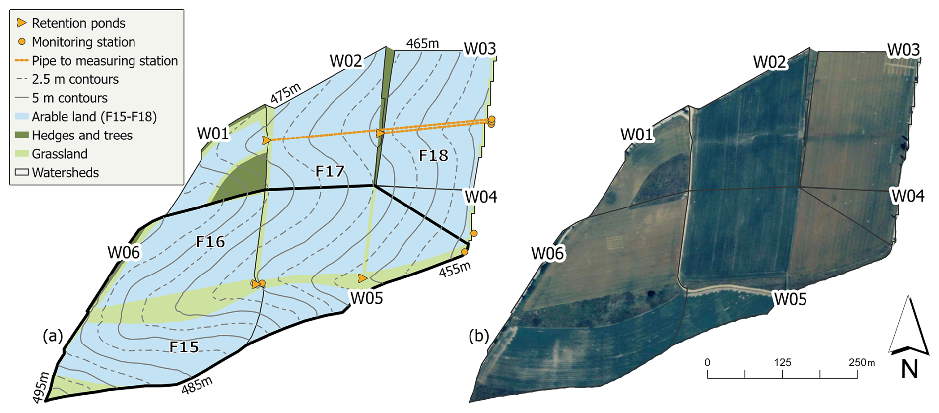
Figure 1 (a) Schematic land use and topography of the experimental farm in Scheyern, Bavaria, with flow direction from west to east. W01–W06 are abbreviations for six watersheds; F15–F18 are the fields located in these watersheds. Note: Watershed W05 (thick line) includes the upslope watershed W06, as W06 is cascading into W05. (b) Aerial photograph of the study area shows the land use patterns and field boundaries on the Scheyern farm in 2002.

Three key conservation practices were implemented to minimise hydrological and sedimentological connectivity: (i) an optimised field layout with reduced field sizes adapted to the steep slopes, (ii) retention ponds at watershed outlets, and (iii) a grassed waterway along the main thalweg of W05 and W06 (Fiener et al., 2019a). The retention ponds were located at the outlets of watersheds W01, W02, W05, and W06 (Fig. 1). Sediment trapping efficiency measurements were conducted for these ponds, revealing an average of 70±14 % (Fiener et al., 2005). Additionally, continuous monitoring systems were installed at the outlet of each micro-scale watershed to measure runoff and sediment yield. The distinction between field-dominated and structure-dominated watersheds will be used consistently throughout this study.

All fields within the watersheds (F15–F18 in Fig. 1) were managed using no-till practices with a crop rotation of winter wheat (Triticum aestivum L.), maize (Zea mays L.), winter wheat, and potatoes (Solanum tuberosum L.). This rotation was staggered across the fields, meaning that while the sequence was identical, the specific crop grown each year varied between fields. After winter wheat, mustard was sown as a cover crop. In the case of potatoes, the mustard was sown into the potato dams built in autumn, while direct seeding into the frost-killed mustard was performed in the following year.

2.2 Erosion monitoring data

The study utilised a unique erosion monitoring dataset acquired between 1994 and 2001. This comprehensive dataset, as well as metadata, are provided by Fiener et al. (2019a). All spatial data were resampled to a consistent 5 m by 5 m grid resolution, matching the digital elevation model (DEM) provided in the dataset (Wilken et al., 2019b). The temporally dynamic input data included daily soil cover measurements and high-resolution precipitation data recorded at 1 min intervals from up to 11 monitoring sites (Wilken et al., 2019a). Additional details regarding these input parameters are provided in Sect. 2.4 below.

For model testing, we used continuous sediment yield data from the six micro-scale watersheds (W01–W06) between 1994 and 2001 (Fig. 1). Runoff and suspended-sediment loads were monitored with a measuring system based on a Coshocton-type wheel sampler (precision ±10 %; Carter and Parsons, 1967; Fiener and Auerswald, 2003). The device continuously diverted an aliquot of approximately 0.5 % from the total flow that left the watersheds through underground-tile outlets with a diameter of 15.6 and 29 cm (Fig. 1) into storage tanks (1.0–3.5 m³). Runoff volumes were measured after each event. Sediment yield was calculated from runoff volumes and sediment concentrations derived from homogenised tank samples dried at 105 °C. At lower rates ($<\mathrm{0.5}\mathrm{L}{\mathrm{s}}^{-\mathrm{1}}$) the system slightly over-estimated runoff, but these small events contributed negligibly to the cumulative water and sediment budgets. Under sampling during very high flows was avoided by (i) employing large wheels (⌀ 61 cm) and (ii) the flow-dampening effect of the retention ponds situated immediately upstream of each outlet (Fiener and Auerswald, 2003).

2.3 Soil erosion modelling

The WaTEM/SEDEM version used in this study consists of two main components: (i) WaTEM, which implements a spatially distributed German adaption of the USLE (Schwertmann et al., 1987; Din-Normenausschuss, 2022), and (ii) SEDEM, which incorporates a transport capacity (TC) equation (Eq. 4) and a routing algorithm for sediment re-distribution based on the DEM (Verstraeten et al., 2002; Van Rompaey et al., 2001; Van Oost et al., 2000). To implement WaTEM/ SEDEM within the GLUE-framework, the original Delphi code-based model was translated to Python 3.12 and was run in PyCharm 2024.1 (Community Edition), which substantially improved computational speed through parallel processing and allowed for easier data handling. To ensure reproducibility and accuracy, we compared the Python implementation against the original Delphi codebase at each individual step of the translation process, verifying that it produced identical outputs for these test cases. Although the Python implementation includes tillage erosion and stream initiation calculations, these components were not utilised in the present study.

The model was applied for the period from April to October of each year from 1994–2001, excluding periods potentially affected by snowmelt erosion and prolonged surface runoff from return flow (Fiener et al., 2019a). While the colder months contributed 10.7 % of the total measured sediment yield (Fiener et al., 2019b), our analysis focused on the dominant water erosion period during heavy rainfall months. Each micro-scale watershed was separately modelled.

2.4 Potential erosion

In contrast to the original WaTEM/SEDEM (Verstraeten et al., 2002; Van Rompaey et al., 2001; Van Oost et al., 2000), in which the USLE factors are derived according to the RUSLE approach (Renard, 1997), we calculated the USLE factors as calculated according to their German adaptation (Eq. 1). This approach is specifically adapted to the soils and climatic conditions of Central Europe and represents the standard methodology for the study region (Schwertmann et al., 1987; Din-Normenausschuss, 2022).

$$\begin{array}{}\text{(1)}& A=R\times K\times \text{LS}\times C\times P,\end{array}$$

where A is the potential erosion ($\mathrm{t}{\mathrm{ha}}^{-\mathrm{1}}{\mathrm{yr}}^{-\mathrm{1}}$), R the rainfall erosivity factor ($\mathrm{N}{\mathrm{h}}^{-\mathrm{1}}{\mathrm{yr}}^{-\mathrm{1}}$), K the soil erodibility factor ($\mathrm{t}{\mathrm{ha}}^{-\mathrm{1}}\mathrm{h}{\mathrm{N}}^{-\mathrm{1}}$), LS the slope length and steepness factor (dimensionless), C the cover management factor (dimensionless), and P the agricultural practices factor (dimensionless).

The high-resolution rainfall data from eleven (1994–1997) and two (1998–2001) precipitation monitoring stations located in the research area were used to calculate the rain erosivity factor (R-factor) (Wilken et al., 2019a). Following the German adaptation of the USLE, rainfall events were considered erosive if they met at least one of two criteria: (i) total rainfall amount≥10 mm (in contrast to the 12.7 mm threshold of the standard USLE, Wischmeier and Smith, 1978) or (ii) maximum 30 min $\text{intensity}\ge \mathrm{10}\mathrm{mm}{\mathrm{h}}^{-\mathrm{1}}$. Individual events were separated by at least 6 h without rainfall (Schwertmann et al., 1987; Din-Normenausschuss, 2022). The calculated rainfall erosivities per monitoring station were interpolated to 5 m by 5 m resolution maps using inverse distance weighting, and the spatially distributed values ranged between 65.90 and 155.10 $\mathrm{N}{\mathrm{h}}^{-\mathrm{1}}{\mathrm{yr}}^{-\mathrm{1}}$ across the eight-year study period.

Soil erodibility (K factor) values were computed following Auerswald et al. (2014) and already provided in the monitoring data set (Auerswald et al., 2019a). The values, originating from a 50 by 50 m sampling grid, were spatially interpolated using ordinary kriging to generate a continuous surface with a 5 m by 5 m resolution grid. The resulting K factor values across the study area ranged from 1.8–4.6 $\mathrm{t}{\mathrm{ha}}^{-\mathrm{1}}\mathrm{h}{\mathrm{N}}^{-\mathrm{1}}$.

The slope length and slope steepness factor (LS factor) was calculated based on the DEM using the approach by Desmet and Govers (1996). When calculating the LS factor for W01, the shrubbed area (Fig. 1) was excluded due to its negligible runoff contribution. Additionally, we calculated the LS factors for W02 and W03 separately from their upslope catchments (i.e. W01 and W02), since their runoff was directed via underground pipes to the monitoring stations (see Fig. 1).

To account for the temporal dynamics of soil protection, we calculated the C factor based on soil cover and rainfall erosivity. This calculation involved deriving continuous daily soil cover data from field measurements, determining the corresponding soil loss ratios (SLR), and weighting these by the seasonal rainfall erosivity.

From 1994–April 1997, bi-weekly crop and residue cover measurements were conducted during growing seasons, with monthly measurements during autumn and spring and additional observations before and after soil management operations. To obtain continuous time series, the point data was linearly interpolated to generate daily cover values (Auerswald et al., 2019b). For the subsequent period (April 1997–2001), we applied standardised daily crop development and residue cover curves, which were derived from the daily crop and residue cover values observed during the detailed monitoring phase in combination with management information (mainly sowing and harvest dates) observed between 1997 and 2001 (Auerswald et al., 2019b; Fiener et al., 2019a). Total soil cover was calculated with residues protecting portions of the otherwise exposed soil according to:

$$\begin{array}{}\text{(2)}& {\text{Co}}_{\text{tot}}={\text{Co}}_{\text{crop}}+(\mathrm{100}-{\text{Co}}_{\text{crop}})\times {\displaystyle \frac{{\text{Co}}_{\text{res}}}{\mathrm{100}}},\end{array}$$

Where Co_tot is the total soil cover (%), Co_crop the cover of the growing crop on the respective field (%), and Co_res the measured soil cover of the residues (%).

Figure 2 illustrates the total soil cover on the respective fields with monthly rainfall erosivity.

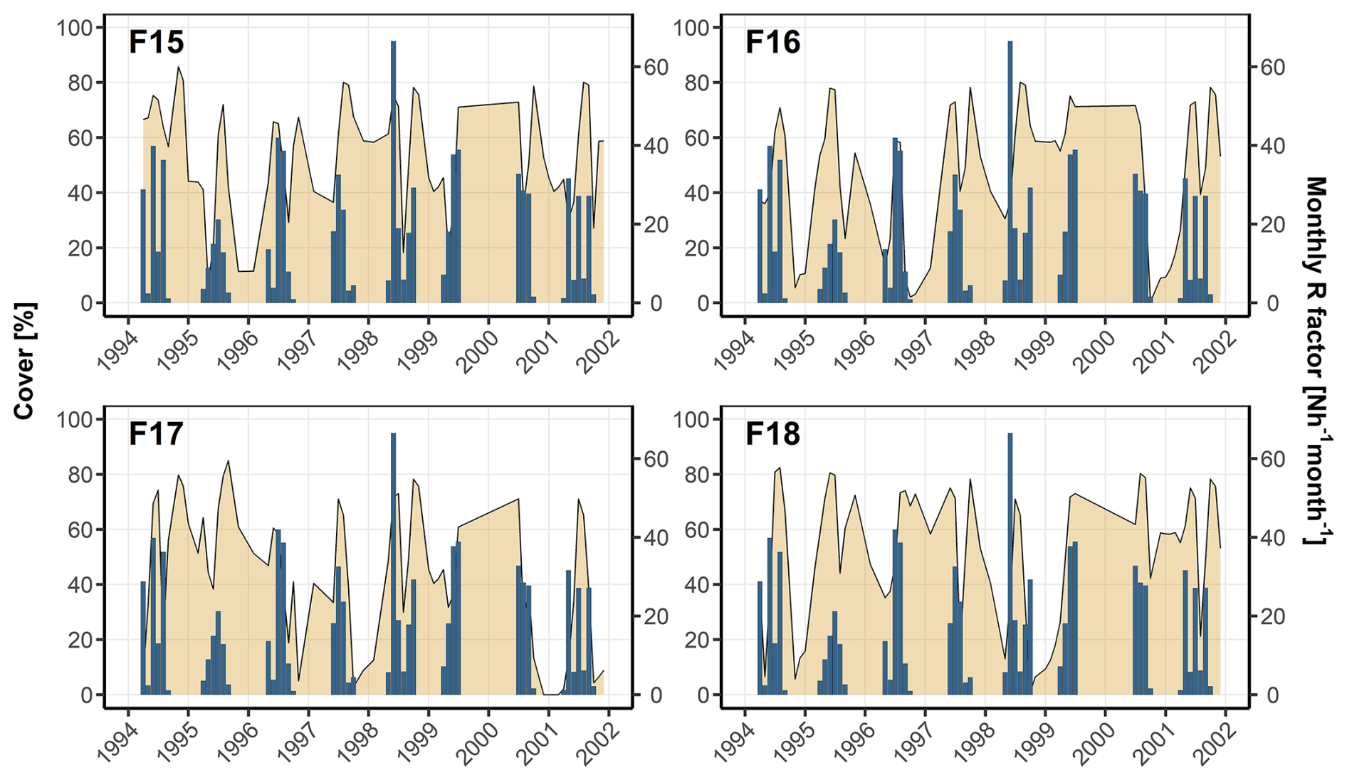
Figure 2 Each field's total soil cover (Residues and crops). Blue bar plots (monthly sum) show monthly R-factors.

The soil loss ratio (SLR) quantifies the protective effect of soil cover by comparing potential soil loss under a given vegetation condition to that under standardised fallow conditions (Schwertmann et al., 1987; Wischmeier and Smith, 1978). While the SLR traditionally considers five crop growth stages, from bare soil (0 % cover) to full canopy coverage (75 %–100 % cover), we also considered crop residue cover. Determining field-specific SLR values involved categorising soil cover into the five growth stages and assigning corresponding SLR values. As no-till was applied at the research farm, lower SLR values were assigned than in conventional systems due to increased soil surface protection. These SLR values were obtained from Schwertmann et al. (1987) and adapted based on our expert knowledge regarding the soil conservation practices in the Scheyern experimental farm (Fiener and Auerswald, 2007; Fiener et al., 2019a).

The annual C factor was calculated by multiplying the monthly proportion of the R factor with the average SLR value of the respective month:

$$\begin{array}{}\text{(3)}& C={\sum }_{\text{month}=\mathrm{1}}^{\mathrm{12}}{\text{SLR}}_{\text{month}}\times R_{\text{prop, month}}\end{array}$$

where C is the cover management factor (dimensionless), SLR_month the average soil loss ratio value of the respective month and R_{prop, month} the proportion of the annual rainfall erosivity factor for the respective month (dimensionless).

Figure 3 shows the annual C and R factor throughout the entire study period.

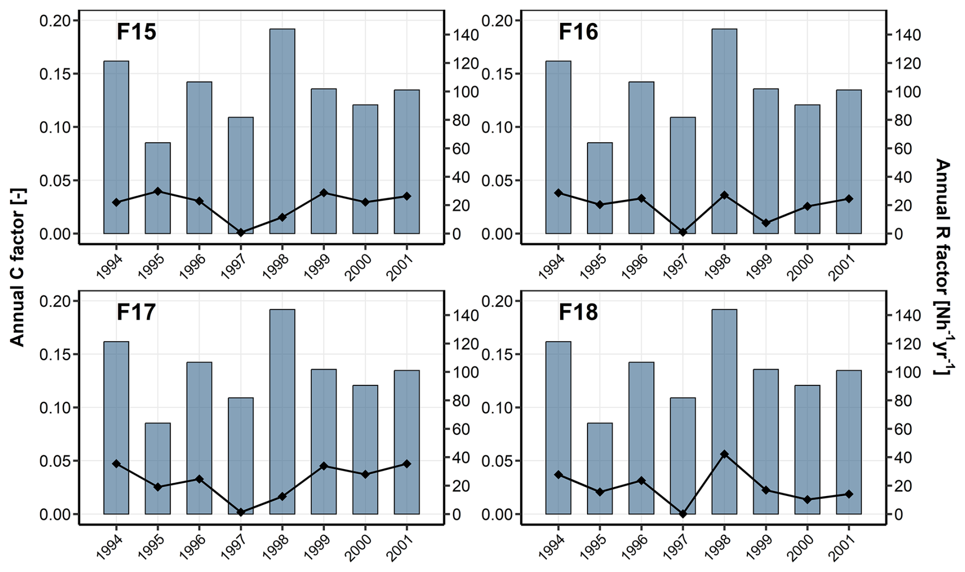
Figure 3 Annual C factor (black dots and lines) and R factor (blue bars) for the individual fields F15–F18 over eight years.

The support practices factor (P factor) was not specifically parametrised for contour-seeding because of field heterogeneity, i.e. not all parts of a single field were contour-seeded, and/or the absence of specific P factor values for structures such as the potato dams. Furthermore, the field geometries often result in high L factors that often exceed the critical slope length limit for effective contouring defined in the German USLE (Schwertmann et al., 1987; Din-Normenausschuss, 2022). Hence, the effective P-factor converges towards 1.0. We accounted for the uncertainty stemming from this lack of parameter representation as part of the model conditioning process (see Sect. 2.4 below).

2.5 Sediment transport and deposition

Transport capacity (TC) quantifies the maximum amount of sediment transported through a grid cell without deposition. When the incoming sediment load into a raster cell exceeds TC, the excess material is deposited within the cell, whilst the remaining portion continues its downstream movement. TC was calculated with the approach proposed by Van Rompaey et al. (2001):

$$\begin{array}{}\text{(4)}& \text{TC}=k_{\text{TC}}\times R\times K\times (\text{LS}-S_{\text{IR}}),\end{array}$$

with

$$\begin{array}{}\text{(5)}& S_{\text{IR}}=\mathrm{4.12}\times S_m^{\mathrm{0.8}}\end{array}$$

where TC is the transport capacity (t ha⁻¹), k_TC the transport capacity coefficient (m) described below, R the rainfall erosivity factor in ($\mathrm{N}{\mathrm{h}}^{-\mathrm{1}}{\mathrm{yr}}^{-\mathrm{1}}$), K is the soil erodibility factor ($\mathrm{t}{\mathrm{ha}}^{-\mathrm{1}}\mathrm{h}{\mathrm{N}}^{-\mathrm{1}}$), LS the slope length and steepness factor (dimensionless), S_IR the interrill slope gradient factor (dimensionless) and S_m the slope (m m⁻¹).

The transport capacity coefficient (k_TC) represents the theoretical upslope distance required for sediment generation to reach maximum TC at a given raster cell under the assumption of uniform slope and erosion conditions (Van Rompaey et al., 2001). The transport capacity coefficient depends on surface roughness and therefore differs according to land use and management. In our model parameterisation, we distinguish between higher values for arable land (k_TC/A) and lower values for grassland (k_TC/G; along field borders and in grassed waterways), which were subjected to the GLUE-based analysis (see Sect. 2.7).

WaTEM/SEDEM's hillslope sediment transport module employs a multiple flow routing algorithm, which distributes sediment from individual cells to their downslope neighbours based on Quinn et al. (1991). The algorithm calculates local slopes to eight neighbouring cells and applies specific weighting factors: 0.50 for orthogonal neighbours and 0.35 for diagonal neighbours. The sediment flux is distributed proportionally to the weighted slope values of all cells at equal or lower elevations.

In this study, we implemented the parcel connectivity (p_con) parameter specifically at field boundaries. p_con reduces the contributing upstream area by a value [%] at these transitions (Notebaert et al., 2006). This reduction has a dual effect: (i) it directly lowers the slope length part of the LS factor, thereby decreasing the potential erosion for subsequent downstream cells, and (ii) it affects TC, which is calculated using the LS factor (Eq. 4). Unlike the original WaTEM/SEDEM version (Notebaert et al., 2006), we implemented p_con within the multiple flow routing algorithm loop calculating the contributing upstream area, ensuring its effects propagate downstream through the flow network. Consequently, the reduction in sediment transport influences the downstream cells and extends to subsequent agricultural fields and vegetated areas. Moreover, we introduced a border deposition (b_dep) parameter, which represents a forced deposition mechanism activated when agricultural field cells contribute sediment to adjacent vegetated areas. Under these conditions, a defined percentage of the transported sediment is deposited directly at the field border within the field.

Retention ponds were implemented within the 5 m by 5 m land use raster map. The locations of the four retention ponds at the outlets of the micro-scale watersheds were mapped, with assigned trapping efficiencies of 54 %, 82 %, 59 %, and 85 % for watersheds W01, W02, W05, and W06, respectively, as measured in Fiener et al. (2005). The standard deviation across all watersheds (±14 %) was applied to account for measurement error in the trapping efficiency values within the GLUE framework (see Sect. 2.6).

2.6 Generalised Likelihood Uncertainty Estimation (GLUE)

We employed the GLUE methodology (Beven and Binley, 1992) to represent model and measurement uncertainties and to identify and analyse behavioural parameter spaces. The GLUE approach recognises that multiple parameter sets may provide equally acceptable simulations of a system within the limitations of a given model structure and observational errors (Beven, 2006).

We established limits of acceptability for the simulated sediment yields by considering multiple sources of uncertainty in the event-based measurements of runoff and sediment concentrations used for calculating annual and mean annual sediment yields. These included Coshocton wheel measurement errors ( ±10 %, Fiener and Auerswald, 2003), runoff collector storage tank sampling errors (estimated ±10 %), and retention pond uncertainties (±14 %). For events with data collection issues (flagged in the data set), we assigned an additional ±50 % error margin. However, for events flagged as “storage tank overflown”, we introduced only an upper error boundary since the measurement taken from the storage tank represents a minimum possible sediment yield during a rainfall event. Finally, we propagated the measurement errors using a Monte Carlo simulation with 1000 realisations and sampling from normal distributions that represented the range of potential errors. The 2.5th and 97.5th percentiles of the resulting aggregated (annual and mean annual) sediment yields were used as the limits of acceptability for simulated values. These uncertainty bounds served as criterion for identifying behavioural model realisations. Hence, only simulations producing outputs within these error margins were classified as behavioural and retained for subsequent analysis.

2.7 Model conditioning and evaluation

The model results were evaluated using R-Studio (R 4.4.2; R-Studio 2024.12.1 Build 563) in two phases to account for the different sediment transport processes in field-dominated and structure-dominated watersheds.

Phase 1 – Field-dominated watersheds

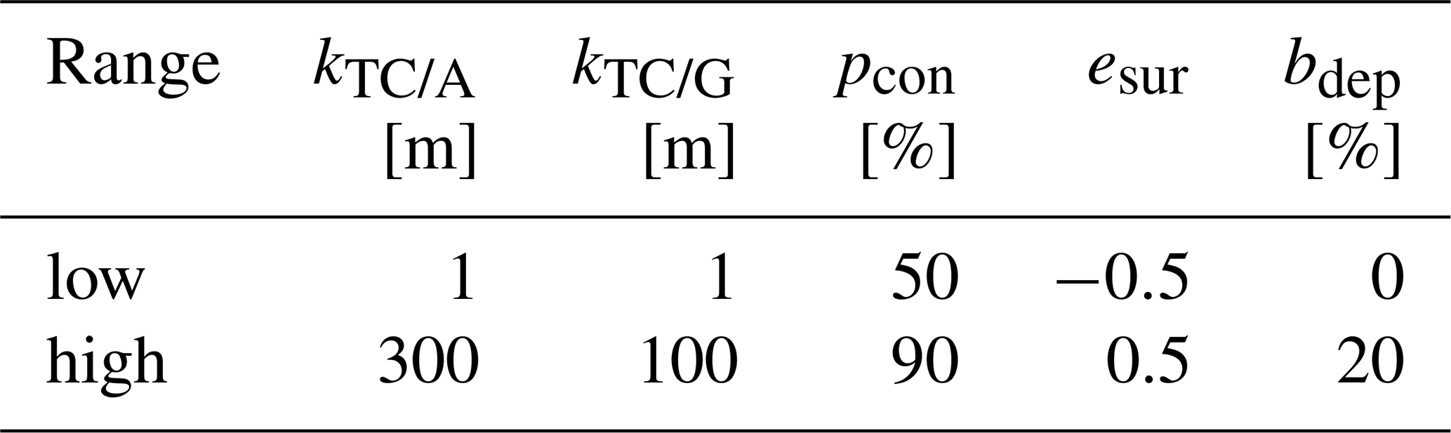
We performed a Monte Carlo simulation with 25 000 realisations for the field-dominated watersheds, sampling parameters from uniform distributions across a priori selected ranges (Table 1). To consider the inherent potential errors in USLE calculations, including uncertainties associated with the parameterisation of the P factor, we modified the potential erosion in individual raster cells through an error surface (e_sur) before routing the sediment. This error surface was sampled from a uniform distribution for each realisation, modifying the USLE-calculated potential erosion (Eq. 1) within a range of 0 to ±0.5:

$$\begin{array}{}\text{(6)}& A_{\text{new},i}=A_i+A_i\times e_{\text{sur}},\end{array}$$

where A_i is the potential soil erosion ($\mathrm{t}{\mathrm{ha}}^{-\mathrm{1}}{\mathrm{yr}}^{-\mathrm{1}}$) calculated by the USLE (Eq. 1) at raster cell i, A_new,i is the potential soil erosion ($\mathrm{t}{\mathrm{ha}}^{-\mathrm{1}}{\mathrm{yr}}^{-\mathrm{1}}$) with incorporated uncertainty at raster cell i, and e_sur the error surface (dimensionless).

Table 1 Parameter ranges used for MC simulation in the WaTEM/SEDEM model. These ranges were selected based on the literature on previous model applications. k_TC/A and k_TC/G are the transport capacity coefficients for arable land and grassland, p_con is the parcel connectivity, e_sur is the error surface and b_dep the border deposition.

The decision to aggregate the uncertainty of the ABAG factors into a single error surface (e_sur), rather than sampling individual factors within the Monte Carlo simulation, stemmed from the nature of our input data. We assumed that parameterisation errors (apart from the P factor) were negligible due to the exceptionally high-quality monitoring data used as input for calculating the ABAG factors (Sect. 2.4). However, as the ABAG is based on regressions that carry residual error, we pragmatically used an error surface to evaluate inherent model biases.

To ensure that k_TC/G is consistently lower than k_TC/A, both were sampled with a constrained relationship, where k_TC/A values were required to be at least 1.5 but no more than 5 times higher than k_TC/G values. Model realisations were classified as behavioural if the simulated sediment yield values fell within the established limits of acceptability (error margins) for the observed data. Likelihoods were calculated only for the spatiotemporal aggregated data for which behavioural model realisations were identified. For these behavioural simulations, we calculated likelihoods by rescaling the mean absolute error (MAE) (Brazier et al., 2000):

$$\begin{array}{}\text{(7)}& L_i={\displaystyle \frac{\mathrm{1}}{{\text{MAE}}_i}}/\sum {\displaystyle \frac{\mathrm{1}}{{\text{MAE}}_i}},\end{array}$$

with

$$\begin{array}{}\text{(8)}& {\text{MAE}}_i=|{\text{Sim}}_i-{\text{Obs}}_i|,\end{array}$$

where L_i is the likelihood of one realisation i (dimensionless), MAE_i is the mean absolute error of realisation i ($\mathrm{t}{\mathrm{ha}}^{-\mathrm{1}}{\mathrm{yr}}^{-\mathrm{1}}$), Sim_i is the simulated values for behavioural runs of realisation i ($\mathrm{t}{\mathrm{ha}}^{-\mathrm{1}}{\mathrm{yr}}^{-\mathrm{1}}$), and Obs_i is the observed sediment value for realisation i ($\mathrm{t}{\mathrm{ha}}^{-\mathrm{1}}{\mathrm{yr}}^{-\mathrm{1}}$).

Phase 2 – Structure-dominated watersheds

For the structure-dominated watersheds, we used the likelihoods associated with behavioural parameter values conditioned in Phase 1 to represent in-field processes (k_TC/A and e_sur) in order to generate another 25 000 realisations. In this second phase, model conditioning was focused on the parameters controlling sediment redistribution through landscape structures (k_TC/G, b_dep and p_con). The same limits of acceptability approach as in phase one was applied to identify behavioural simulations. We calculated new likelihood values for these simulations to analyse their performance in representing structural erosion control practices.

2.8 Spatiotemporal model evaluation

Model outputs were evaluated at multiple spatiotemporal scales through sequential aggregation steps to analyse short-term dynamics against its intended long-term design: First, we temporally aggregated the sediment yields by calculating eight-year means for each individual watershed. Second, we spatially aggregated the simulated sediment yields by calculating their means for each watershed group (field- and structure-dominated), but keeping an annual resolution. Third, eight-year means for each watershed group were calculated (spatial and temporal aggregation).

To further analyse relative errors, the percent bias (PBIAS) was calculated by:

$$\begin{array}{}\text{(9)}& \text{PBIAS}=\left({\displaystyle \frac{{\text{Sim}}_i-{\text{Obs}}_i}{{\text{Obs}}_i}}\right)\times \mathrm{100},\end{array}$$

Where Sim_i is the simulated values for behavioural realisation i ($\mathrm{t}{\mathrm{ha}}^{-\mathrm{1}}{\mathrm{yr}}^{-\mathrm{1}}$), and Obs_i is the observed sediment value for realisation i ($\mathrm{t}{\mathrm{ha}}^{-\mathrm{1}}{\mathrm{yr}}^{-\mathrm{1}}$).

2.9 Spatial analysis

Spatial analysis was performed using R-Studio (R 4.4.2; R-Studio 2024.12.1 Build 563). To quantify the spatial distribution of sediment yield and the associated uncertainty, the cell-wise mean and standard deviation were calculated across all behavioural model realisations.

3 Results

3.1 Model performance across scales

The modelled annual sediment yields for field-dominated watersheds (W01–W04) were within the same order of magnitude of the measurements. However, the model was not considered behavioural for predicting annual sediment yields according to our pre-established acceptability criterion. The simulated annual sediment yields were predominantly overestimated (22 out of 32 cases; Fig. 4a–d), occasionally underestimated (4 out of 32 cases; in the year 1997 and 2000 in W01; 1994 in W02; 1994 in W04; Fig. 4a, b and d), with only a small portion of simulations overlapping the observational data (6 out of 32 cases; Fig. 4a–d). The tendency to overestimate sediment yield is more pronounced in watersheds W05 and W06. Only in 1994 the model had the tendency to underestimate measured sediment yields in watershed W05 (Fig. 5b). In W06, measured sediment yields were the lowest among all watersheds (maximum of 0.02 $\mathrm{t}{\mathrm{ha}}^{-\mathrm{1}}{\mathrm{yr}}^{-\mathrm{1}}$ in 2000), with zero sediment yield measurements in 1995, 1997, and 2001, yet the model consistently overestimated sediment yield across all years in this watershed.

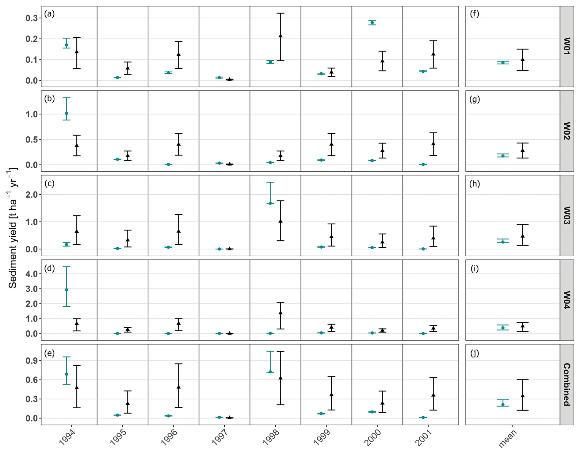
Figure 4 Annual and eight-year mean sediment yields in field-dominated watersheds. (a–d) Annual sediment yields: Black triangles indicate the mean and the full range from 25 000 model realisations (black whiskers), while cyan dots represent mean measured sediment yields with computed error ranges (cyan whiskers). (f–i) The watershed-specific eight-year mean measured sediment yields (cyan) and eight-year mean simulated yields (black). (e) Spatially combined annual watershed sediment yields. (j) Spatially aggregated eight-year mean yields. Note: In some years (e.g., 1998), cyan whiskers show larger uncertainties above the mean values; this is because storage tank overflow contributes only to higher uncertainties (see Sect. 2.6).

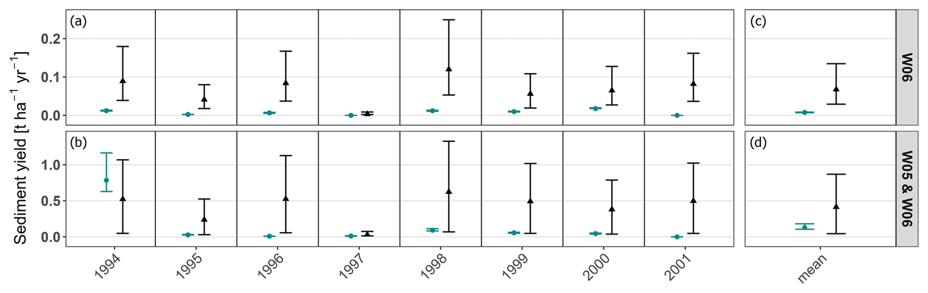
Figure 5 Annual and eight-year mean sediment yields in structure-dominated watersheds. (a, b) Annual sediment yields: Black triangles indicate the mean and the full range from 25 000 model realisations (black whiskers), while cyan dots represent mean measured sediment yields with computed error ranges (cyan whiskers). (c, d) The watershed-specific eight-year mean measured sediment yields (cyan) and eight-year mean simulated yields (black).

When evaluated using eight-year mean values per watershed, simulations showed better agreement with observations. The temporal aggregation revealed varying proportions of behavioural model realisations across individual watersheds. W04 had the highest amount with 69 % of all realisations, while other watersheds exhibited lower proportions (W01: 13 %, W02: 22 %, W03: 22 %). W05 exhibited minimal behavioural realisations of 1 %. In W06 (Fig. 5c), none of the actual model realisations matched the observational data including measurement errors. Furthermore, no common behavioural realisations were found across all watersheds, indicating that each watershed had a different behavioural parameter space. The analysis of the spatially aggregated watersheds (field-dominated vs. structure-dominated), while maintaining annual temporal resolution, revealed behavioural model realisations in some years but not consistently throughout the entire eight-year period for each watershed group (Fig. 4e and b).

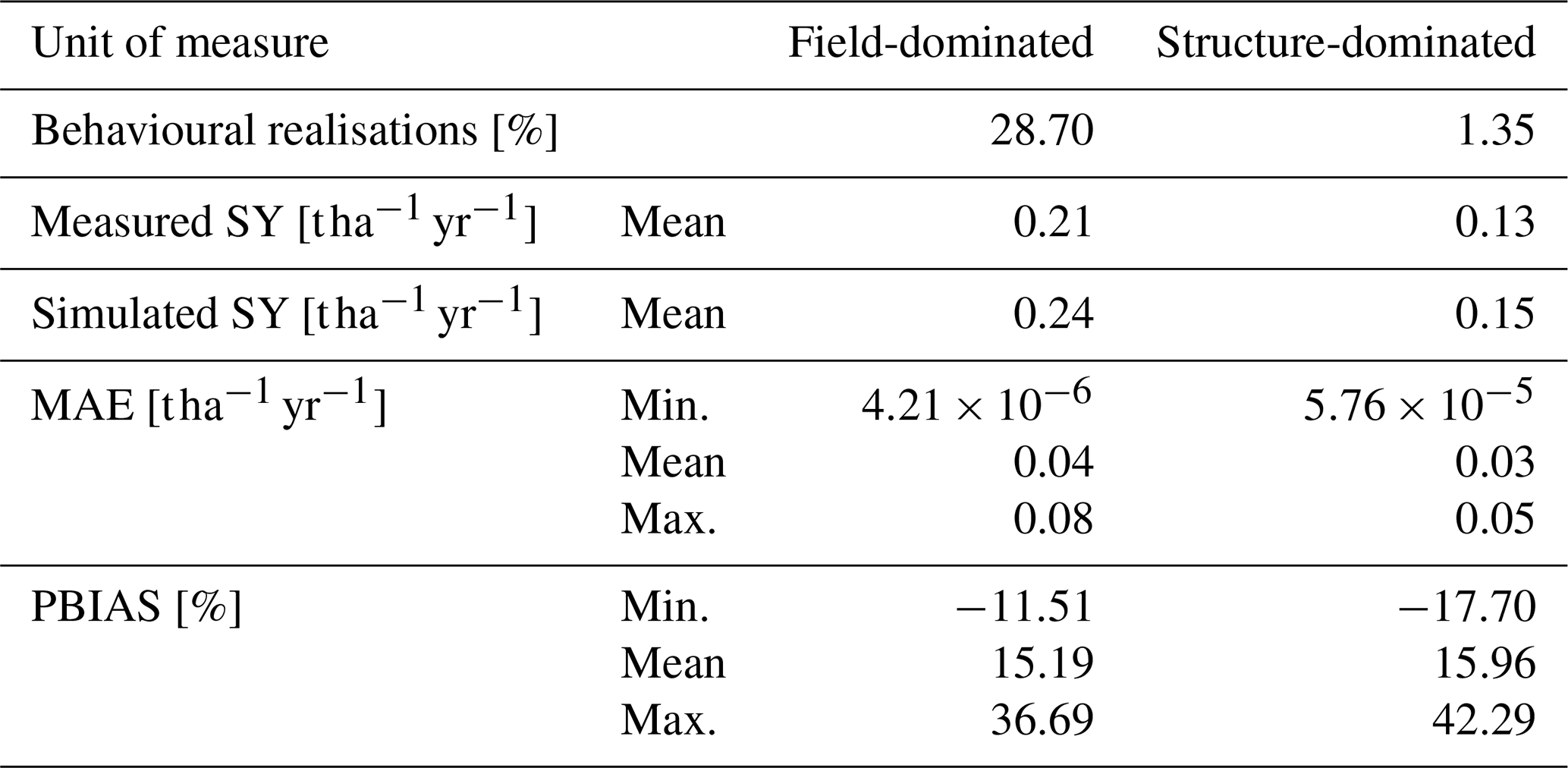
When combining both spatial and temporal aggregation, behavioural realisations were generated for each watershed group (Figs. 4j and 5d). Across the entire set of 25 000 realisations, the mean MAE values were 0.14 $\mathrm{t}{\mathrm{ha}}^{-\mathrm{1}}{\mathrm{yr}}^{-\mathrm{1}}$ for field-dominated watersheds and 0.29 $\mathrm{t}{\mathrm{ha}}^{-\mathrm{1}}{\mathrm{yr}}^{-\mathrm{1}}$ for structure-dominated watersheds, with maximum MAE values of 0.40 $\mathrm{t}{\mathrm{ha}}^{-\mathrm{1}}{\mathrm{yr}}^{-\mathrm{1}}$ and 0.74 $\mathrm{t}{\mathrm{ha}}^{-\mathrm{1}}{\mathrm{yr}}^{-\mathrm{1}}$, respectively. Table 4 presents the model performance metrics specifically for the subset of behavioural model realisations within the watershed groups. The eight-year mean modelled sediment yield across field-dominated watersheds (W01–W04) was 0.35 $\mathrm{t}{\mathrm{ha}}^{-\mathrm{1}}{\mathrm{yr}}^{-\mathrm{1}}$ , compared to the measured eight-year mean of 0.21 $\mathrm{t}{\mathrm{ha}}^{-\mathrm{1}}{\mathrm{yr}}^{-\mathrm{1}}$ . For structure-dominated watersheds W05 and W06, we simulated an eight-year mean of 0.41 $\mathrm{t}{\mathrm{ha}}^{-\mathrm{1}}{\mathrm{yr}}^{-\mathrm{1}}$ (Fig. 5c and d), against a measured mean of 0.13 $\mathrm{t}{\mathrm{ha}}^{-\mathrm{1}}{\mathrm{yr}}^{-\mathrm{1}}$ . The 1994 sediment yield peak in W05 strongly influenced the system's overall performance, ultimately leading to an increased number of behavioural model realisations when evaluated across the entire period (Fig. 5d).

Table 2 Comparison of model performance metrics between micro-scale watershed groups based on eight-year mean of behavioural realisations, including mean sediment yield (SY) as well as error statistics (MAE, PBIAS) with maximum (Max.), minimum (Min.) and mean values.

3.2 Behavioural parameter space

We analysed the behavioural parameter space for the spatially and temporally aggregated model outputs, as only this aggregation level yielded behavioural realisations for both field-dominated and structure-dominated watershed groups.

For field-dominated watersheds, the analysis focused on the error surface and in-field parameter e_sur and k_TC/A. While behavioural realisations were identified across the entire ranges of all parameters, higher likelihood values concentrated in specific regions. Specifically, e_sur values closer to −0.5 exhibited higher likelihood values than lower e_sur values (Fig. 6b). In contrast, k_TC/A showed no discernible pattern across the response surface (Fig. 6c). The relationship between these parameters revealed a clear compensation mechanism, where lower k_TC/A values required higher e_sur values to produce behavioural realisations (Fig. 6a).

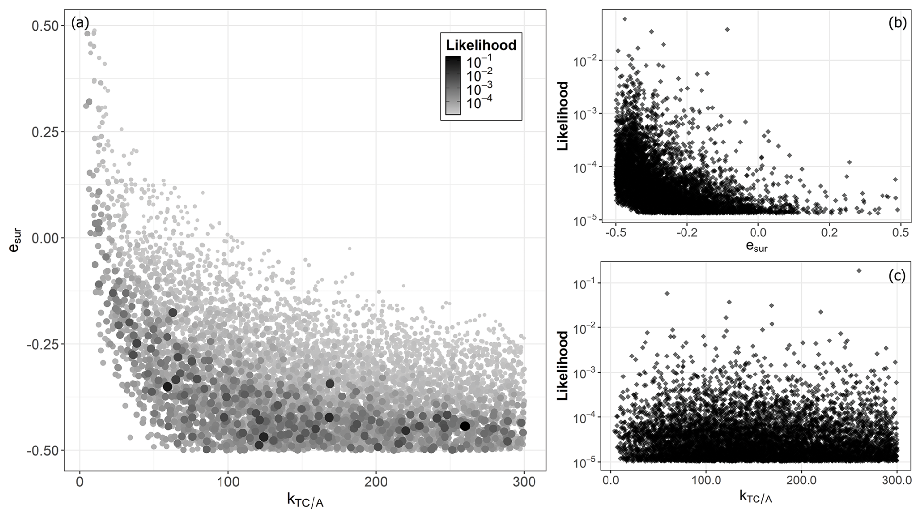
Figure 6 Parameter likelihoods across field-dominated micro-scale watersheds, showing only behavioural model realisations. (a) The relationship between e_sur and k_TC/A parameters. Circle size and shade intensity indicate the likelihood of each parameter combination, with larger and darker circles representing higher likelihood values. (b) The relationship between likelihood and e_sur. (c) The relationship between likelihood and k_TC/A.

In structure-dominated watersheds, the analysis focused on parameters controlling sediment transport and deposition in grasslands and landscape structures (k_TC/G, b_dep, and p_con). The k_TC/G parameter exhibited a distinct likelihood peak between approximately 9 and 11 m, with behavioural values ranging from approximately 7.5–15 m (Fig. 7a), which is notably narrower than the sampled range of up to 150 (Table 1). In contrast, b_dep and p_con displayed relatively uniform likelihood distributions across their entire ranges (Fig. 7b and c). When plotting b_dep against p_con, homogeneous likelihood distributions emerged with no apparent dependencies (Fig. 7f). Examinations of b_dep and p_con against k_TC/G revealed a horizontal band of high likelihood values at specific k_TC/G values, without any directional trends (Fig. 7d and e).

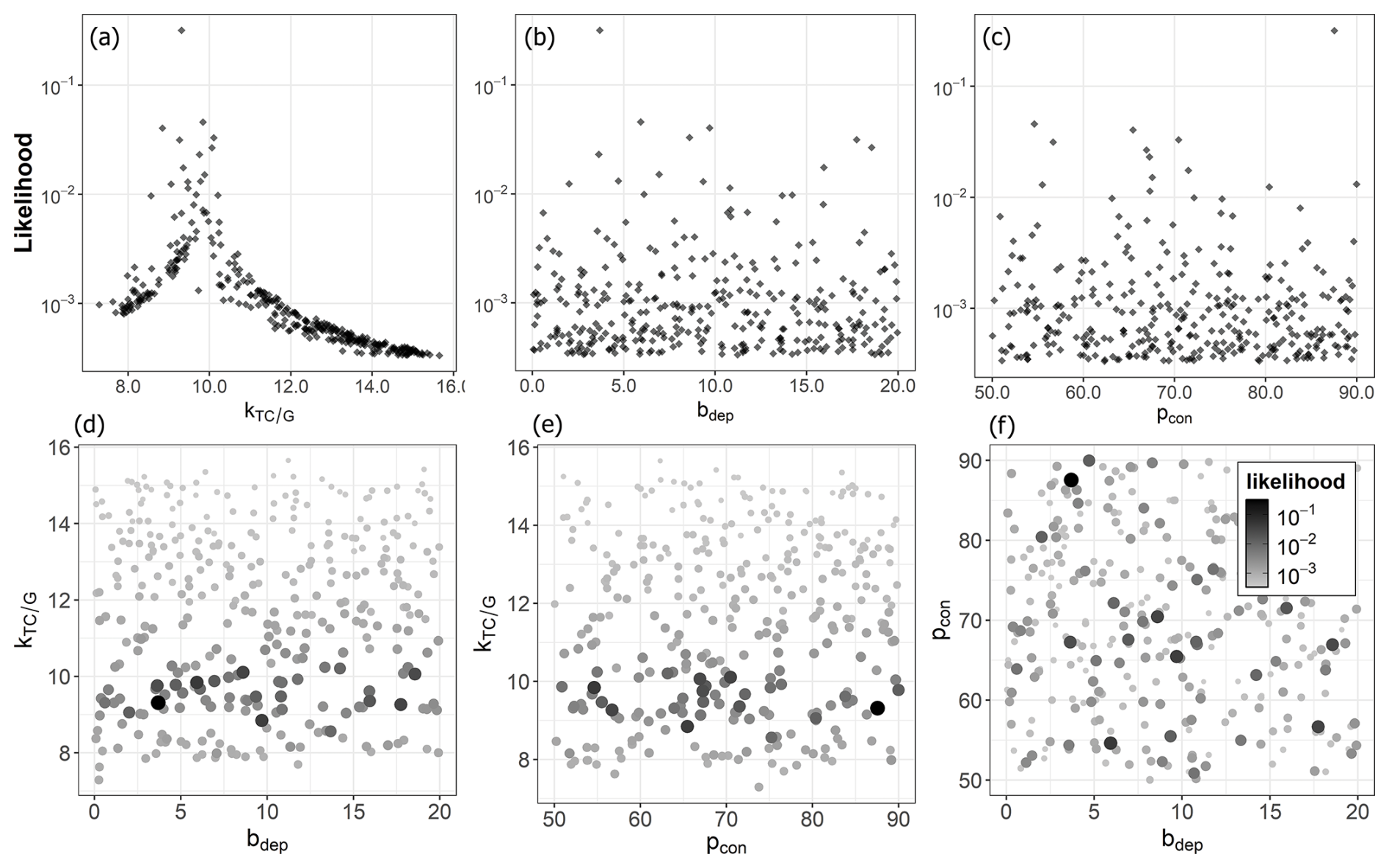
Figure 7 Parameter likelihoods across structure-dominated micro-scale watersheds, showing only behavioural model realisations. (a) The relationship between likelihood and k_TC/G. (b) The relationship between likelihood and b_dep. (c) The relationship between likelihood and p_con. (d) The relationship between b_dep and k_TC/G. Circle size and colour intensity indicate the likelihood of each parameter combination, with larger and darker circles representing higher likelihood values. (e) The relationship between p_con and k_TC/G. (f) The relationship between b_dep and k_TC/G.

3.3 Spatial analysis

In field-dominated watersheds, substantial deposition was primarily confined to retention ponds, while other areas outside arable lands showed minimal deposition, except for W03 (Fig. 8a). In W04, negligible to no deposition was observed. Conversely, structure-dominated watersheds exhibited considerably more intense erosion-deposition dynamics. The grassed waterway showed a clear deposition pattern, with W06 exhibiting the most pronounced deposition patterns leading toward the retention pond at the outlet.

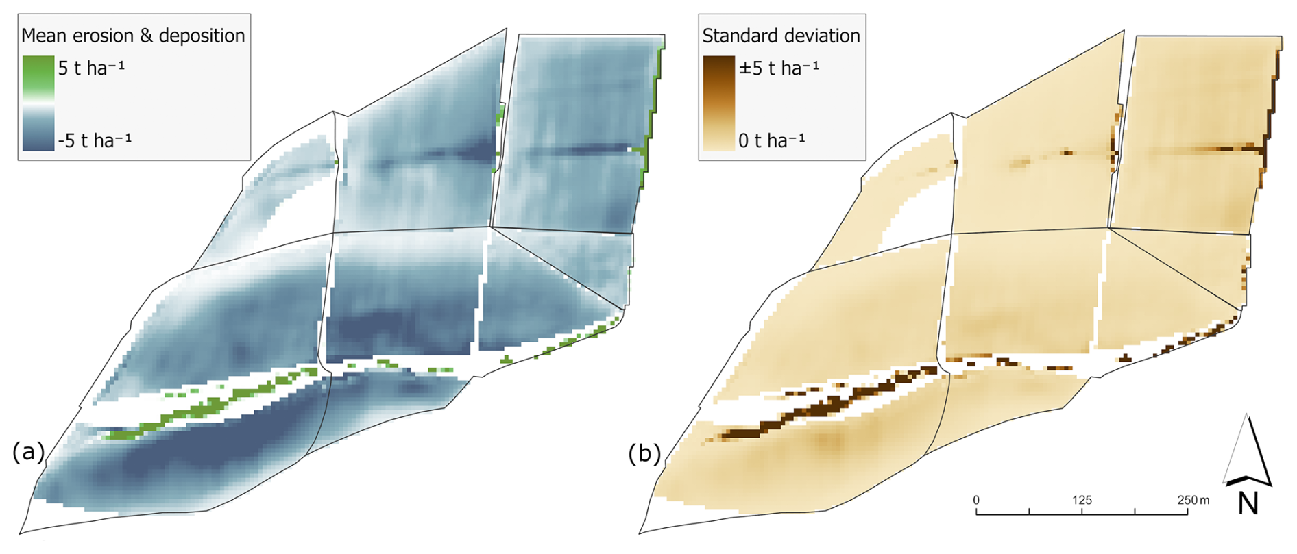
Figure 8 (a) The mean of simulated potential erosion and deposition of behavioural model realisations over the eight-year period. Negative values indicate erosion and positive values deposition. (b) The cell-wise standard deviation of behavioural model realisations over the eight-year period.

The map of the standard deviation (Fig. 8b) also displays a spatial shift in model uncertainty between the two watershed groups. In field-dominated watersheds, standard deviation exhibits concentrations along in-field flow pathways, the retention ponds and the small structures next to their outlets. In structure-dominated watersheds a substantial increase in standard deviation is visible along the flow pathways towards and along the grassed waterway.

4 Discussion

4.1 GLUE framework and uncertainties

We tested WaTEM/SEDEM using a limits of acceptability approach within the GLUE framework. For this, we implemented a two-phase procedure, first conditioning and evaluating field-dominated watersheds, and then using the behavioural parameter space of these watersheds to condition and evaluate structure-dominated systems. Alatorre et al. (2010) demonstrated that soil erosion models often exhibit parameter compensation effects, where different parameter combinations produce similar outputs at the catchment scale – a manifestation of the equifinality concept (Beven, 2006). Our sequential approach helped to minimise these effects by first constraining the simulated erosion (k_TC/A and e_sur) in field-dominated watersheds and then conditioning the transport parameters (k_TC/G, p_con and b_dep) in more complex systems.

The limits of acceptability approach incorporated multiple sources of measurement uncertainty. Nearing (2000) demonstrated through replicated plot studies that natural variability in erosion measurements is particularly pronounced for low-magnitude erosion events, such as the ones observed in this study. While Nearing (2000) proposed a quantitative method for estimating the expected variability of erosion measurements, his approach is specifically developed for plot-scale studies and cannot be extrapolated to watersheds or more complex landscape systems. Given the (to the best of our knowledge) current absence of methodologies for determining error boundaries for low sediment yield measurements at larger scales, we necessarily relied on relative error estimates. An implementation of proper measurement variability-derived error ranges would likely result in a substantially higher number of behavioural model realisations, particularly for low sediment yield measurements where the variability is the highest (Nearing, 2000). This reveals the need for developing robust approaches for defining limits-of-acceptability criteria for sediment yield estimates that account for the full range of uncertainties, e.g. instrument precision, sampling errors, data processing, or site-specific variations.

Erosion models typically exhibit systematic biases, overpredicting low sediment yields while underpredicting high sediment yields (Nearing, 1998; Risse et al., 1993; Kinnell, 2007). This is particularly relevant for our study area, where the implemented watershed-wide soil conservation and sediment trapping resulted in a measured mean sediment yield of only 0.16 $\mathrm{t}{\mathrm{ha}}^{-\mathrm{1}}{\mathrm{yr}}^{-\mathrm{1}}$, which is substantially lower than erosion rates typically range between $\mathrm{3}-\mathrm{10}\mathrm{t}{\mathrm{ha}}^{-\mathrm{1}}{\mathrm{yr}}^{-\mathrm{1}}$ in the Bavarian Tertiary hill region (Auerswald et al., 2009). To investigate the modelling under/over prediction issue, we used an error surface (e_sur) multiplied with the erosion calculated by the USLE (Eq. 6). The analysis of behavioural model realisations revealed a concentration of likelihood values near small e_sur values, reducing sediment by up to 50 % (Fig. 6b). This indicates that in our study WaTEM/SEDEM overestimates soil erosion in landscapes with implemented conservation practices. This is also evident looking at Figs. 3a–d and 4a, b, which illustrate a general tendency for overestimation of modelled sediment yields in all watersheds.

4.2 Model performance and limitations

WaTEM/SEDEM correctly simulated the magnitude of the very low sediment yields in micro-scale watersheds optimised for soil conservation and reduced sediment transport, with annual values closely aligning with measured data (Figs. 4a–d and 5a, b). Nonetheless, the model did not consistently meet our limits of acceptability for annual realisations and therefore was rejected for making precise annual simulations. The model's performance improved notably when applied to longer-term means and larger spatial units, where more behavioural model realisations were identified.

4.2.1 Field-dominated watersheds

The model simulated the very low sediment yields resulting from well-established in-field soil conservation practices in field-dominated watersheds, comparable to the measured data. In general, observed sediment yields were overestimated, which can be attributed primarily to difficulties in accurately representing this conservation system, particularly unique practices such as mustard sown onto autumn-built dams where potatoes were later directly planted (Fiener and Auerswald, 2003). Such unconventional approaches are not adequately captured in the SLR values for no-till systems as evaluated in the German adaptation of the USLE (ABAG; Schwertmann et al., 1987; Din-Normenausschuss, 2022), even with the use of very low soil loss ratios in the parameterisation of the C factor, which represent the continuous soil cover through the crop rotation in the experimental farm (Fig. 2).

Conversely, the model underestimated sediment yields in some years because even optimally managed conservation systems experience short time windows with weak protection. During these short windows with reduced soil protection (Fig. 2), substantial erosion events may occur, like in systems not under soil conservation. In general, erosion processes are typically dominated by extreme events (Gonzalez-Hidalgo et al., 2012; Steegen et al., 2000), as exemplified in our study by an April 1994 rainfall event of 114 mm within 66 h coinciding with low soil coverage in W02 (Fig. 2), accounting for approximately 58 % of that year's total sediment yield (see year 1994 in Fig. 4b). The model's annual time step fails to capture these critical temporal coincidences, a structural limitation that becomes more pronounced when such events are infrequent. This temporal limitation aligns with findings by Risse et al. (1993), who demonstrated that USLE's model efficiency diminishes at the annual scale. When averaging over the eight-year study period, these extreme events are smoothed out, which explains the model's improved performance at longer timescales (Table 2). This deficit could not be compensated using high-resolution input data (daily soil cover, high resolution and on-site rainfall measurements). However, it is important to note that the episodic nature of erosion is always difficult to capture even with event-based models, and hence aggregation over time tends to improve any kind of erosion model. This is especially true if events are rare and the overall erosion values are small (Nearing, 1998). Future studies could employ synthetic data generation (Srikanthan and Mcmahon, 2001), allowing for an assessment of the model's sensitivity beyond our high-resolution input data.

For the temporally aggregated eight-year means, there was no single parameter set that produced behavioural model realisations across all field-dominated watersheds simultaneously when applying our limits of acceptability criterion. This indicates a limitation in parameter transferability within our study context. While Van Rompaey et al. (2001) recognized technical limitations of WaTEM/ SEDEM in model transferability related to grid size and routing methods, our findings suggest additional challenges in accurately representing processes within micro-scale watersheds with specific in-field soil conservation practices (e.g. no-till farming). The need for watershed-specific calibration, even within relatively homogeneous landscapes with similar crop and soil properties, indicates that parameter calibration compensates for inherent model or data limitations. At such fine scales, WaTEM/SEDEM may struggle to accurately represent the complex interactions between soil conservation practices and erosion processes. However, it is important to note that these difficulties may stem from the low-magnitude nature of the erosion events observed in our study. As demonstrated in paired-plot experiments, natural variability is higher for small events (Wendt et al., 1986). Therefore, areas with higher erosion rates typically yield data that is less noisy and inherently easier for models to reproduce (Nearing, 1998).

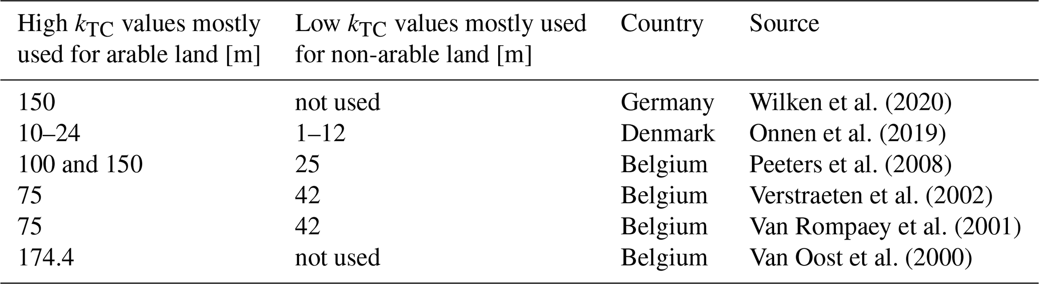
Similar calibration challenges seem to exist more broadly in WaTEM/SEDEM applications across different landscape types and research questions, as evidenced by a wide range of calibrated k_TC values reported across different studies (Table 3), with k_TC/A values varying from 10–174.4 m. As Beven (2006) argues, such calibration approaches may achieve mathematical fitting while concealing fundamental model inadequacies.

4.2.2 Structure-dominated watersheds

Unlike field-dominated watersheds, structure-dominated systems demonstrated different response patterns to extreme erosion events. In these watersheds, sediment generated during individual large erosion events (as observed in the field-dominated watersheds), is predominantly captured by grassed waterways and retention ponds (Fiener and Auerswald, 2003, 2005), thus reducing the variability of event sediment yields. This buffering effect explains why the model consistently overestimates sediment yield across all years for structure-dominated watersheds (Fig. 5a and b), in contrast to the occasional underestimation observed in field-dominated systems (Fig. 4a–d).

Only one exception to this pattern was observed: the model underestimated sediment yield in W05 during 1994, when the lower part of the grassed waterway required reseeding after losing its initial grass cover along the thalweg during a spring erosion event (Fiener and Auerswald, 2003). This exceptional case quantitatively demonstrates the role of functional grassed waterways, as the measured sediment yield in 1994 for W06 was substantially higher (0.78 $\mathrm{t}{\mathrm{ha}}^{-\mathrm{1}}{\mathrm{yr}}^{-\mathrm{1}}$) than in subsequent years when the grassed waterway was fully established (averaging only 0.03 $\mathrm{t}{\mathrm{ha}}^{-\mathrm{1}}{\mathrm{yr}}^{-\mathrm{1}}$ from 1995–2001), representing an approximately 96 % reduction in sediment yield (Fig. 5b).

The model's systematic overestimation of sediment yields in structure-dominated watersheds reveals limitations in representing the sediment trapping mechanisms of grassed waterways. The primary limitation is the model's inability to capture re-infiltration processes within the grassed waterway, which is not accounted for in WaTEM/SEDEM's transport capacity formulation. Fiener and Auerswald (2005) demonstrated that grassed waterway effectiveness depends strongly on morphological characteristics, particularly the cross-sectional shape, with flat-bottomed waterways showing substantially higher runoff reduction. The infiltration increases with length and flatter cross-sections of grassed waterways, which provide larger runoff widths and consequently greater infiltration areas. A previous study showed that in the upper part of the grassed waterway (W06), where WaTEM/SEDEM more substantially underestimates the sediment trapping, the long-term runoff and sediment yield reductions were respectively about 90 % and 97 %, while it was about 10 % and 77 % in the lower part of the grassed waterway (W05) with a ditch-like cross-section (Fiener and Auerswald, 2003).

4.3 Spatial dynamics of erosion and deposition

The main reason for the reduction of sediment yield at the outlet within structure-dominated watersheds is visible in the eight-year mean map of behavioural model realisations (Fig. 8a). Depositional patterns are prominent along the flux pathway of the grassed waterway, particularly in W06. Because WaTEM/SEDEM is sensitive to the parameter controlling deposition inside these soil conservation structures (k_TC/G), the standard deviation in these areas is exceptionally high (Fig. 8b).

However, high uncertainty is not limited to the grassed waterways. It is also evident in depositional areas of field-dominated watersheds (most pronounced in W03). This suggests that deposition is generally prone to high uncertainties, regardless of the dominant structures. Furthermore, field-dominated watersheds exhibit high standard deviations within the fields themselves. This likely stems from parameter uncertainty regarding sediment supply, specifically the error surface parameter (e_sur, see Fig. 6b), which directly influences the sediment supply generated within the arable land.

4.4 Spatial aggregation

For the structure-dominated watersheds, spatial aggregation was critical for overcoming watershed-specific model failures. While the model failed to produce any behavioural realisations for W06 (even temporally lumped), the spatially aggregated group achieved 1.35 % behavioural realisations. This aligns with the scale-dependency concepts reviewed by De Vente and Poesen (2005), who note that process dominance shifts with spatial scale, often allowing models to perform adequately at larger scales even if they miss finer processes.

For field-dominated watersheds, the spatial aggregation acted primarily as an averaging of varying crop states, smoothing out the heterogeneity of cover conditions, and any given watershed peculiarities. In contrast, for structure-dominated watersheds, spatial aggregation facilitates the identification of behavioural parameter spaces by masking local structural inadequacies, such as the deposition dynamics in grassed waterways. Consequently, the differences between spatially aggregated field-dominated and structure-dominated watersheds can be attributed to their structural components.

Table 3 Comparison of k_TC parameter values of behavioural model realisations used in different studies with WaTEM/SEDEM.

4.5 Distribution of behavioural model parameter values

The TC within agricultural fields is primarily controlled by the transport coefficient k_TC/A (Van Rompaey et al., 2001). Lower k_TC/A values reduce TC, promoting in-field deposition and consequently decreasing sediment yield at the watershed outlet. Our analysis revealed behavioural model realisations across the full a priori selected range of k_TC/A values, with no clear pattern for field-dominated watersheds, demonstrating no sensitivity even at very low k_TC/A values near 1 or very high e_sur values of 0.5 (Fig. 6a). This lack of sensitivity may be attributed to the retention ponds in W01 and W02 and the very low simulated erosion values. Since TC remained sufficiently high to transport the low sediment fluxes even with very low k_TC/A values, sediment transport is thus supply-limited rather than constrained by transport capacity within the fields.

The low transport capacity coefficient for rougher surfaces, in case of this study for grassland k_TC/G, usually triggers deposition in these areas (Van Rompaey et al., 2001). Our analysis identified behavioural values for k_TC/G between approximately 7.5–15 m with a notable likelihood spike between approximately 9 and 11 m, relatively low values compared to other studies (Table 3). While Onnen et al. (2019) reported similarly low values for Danish landscapes, they explicitly attributed this to sandy soils in Denmark. However, our study area features predominantly silt loam and loamy soils, which are much more comparable to the Belgian soils (Table 3) where low k_TC values for rough surfaces were implemented (Peeters et al., 2008; Verstraeten et al., 2002; Van Rompaey et al., 2001).

These low k_TC/G values can have some possible interpretations: (i) most likely, the model is compensating for its inability to represent re-infiltration processes in grassed waterways, and/or (ii) the model may partly compensate for an overestimation of erosion rates in the draining fields. However, although the model outputs are fully spatially distributed (Fig. 8), it is not possible to compare the simulated patterns with spatially distributed observational data (e.g. aerial images, field surveys), because, except for some rare larger events, the effective soil conservation established prevents visible erosion features like rills.

In our study, WaTEM/SEDEM showed no sensitivity to parameters b_dep and p_con that represent the influence of linear landscape features. These parameters displayed homogenous likelihood distributions across the sampled parameter space (Fig. 7b and c). This lack of sensitivity could stem from several factors: (i) sampling an overly narrow parameter space, (ii) limited influence of field borders in the studied watersheds due to the layout of the fields and watersheds with a small number of border situations, and/or (iii) a dominance of k_TC/G implemented over a long grass structure, which may nullify the influence of b_dep and p_con in the model outputs, especially in watershed W05 and W06.

An additional limitation of the current parameterisation approach, particularly for grassed waterways, is its static nature. The effectiveness of grassed waterways and retention structures varies throughout the year due to seasonal vegetation changes (Fiener and Auerswald, 2003). Additionally, there is an important interaction between sediment influx and trapping efficiency – as influx increases, the relative trapping efficiency typically decreases (Dermisis et al., 2010; Fiener and Auerswald, 2018). Dermisis et al. (2010) demonstrated this inverse relationship, showing that grassed waterway trapping efficiency decreases as peak runoff discharge increases, with notable breakpoints in efficiency between different flow rates. The current static connectivity and transport capacity parameters (p_con, b_dep and k_TC/G) cannot adequately capture these temporal variations and flux-dependent relationships, suggesting the need for a more dynamic parameterisation approach that accounts for both seasonal changes and influx response if the model is applied to an annual time-step.

5 Conclusion

We evaluated WaTEM/SEDEM's capability to simulate sediment yields in micro-scale watersheds optimised for soil conservation and sediment transport reduction using a limits-of-acceptability approach within the GLUE framework. Our investigation examined model performance across different levels of spatiotemporal data aggregation and analysed the sensitivity of the model's response surface to the variability in the behavioural parameter space. Moreover, we used a two-step conditioning process, in which model parameters linked to in-field erosion processes were conditioned in field-dominated watersheds and later applied in structure-dominated watersheds, for which a separate set of connectivity parameters was also conditioned.

The model was unable to produce behavioural realisations for watersheds optimised for soil conservation and sediment transport reduction at annual time steps based on our strict limits of acceptability criterion despite the small absolute prediction errors over all model realisations (eight-year $\text{MAE}=\mathrm{0.14}\mathrm{t}{\mathrm{ha}}^{-\mathrm{1}}{\mathrm{yr}}^{-\mathrm{1}}$ for field-dominated and eight-year $\text{MAE}=\mathrm{0.29}\mathrm{t}{\mathrm{ha}}^{-\mathrm{1}}{\mathrm{yr}}^{-\mathrm{1}}$ for structure-dominated watersheds). For the field-dominated watersheds, the model particularly struggled with simulating annual sediment yields. This is because soil conservation practices reduced the number of erosion events, yet some events (e.g., after potato harvest) retained a similar magnitude as in conventional cultivation.

Aggregating model outputs in time and space worked best for field-dominated systems, which compensated for the underestimation of soil conservation in controlling soil erosion and the model's inability to capture extreme events within an annual time step. While WaTEM/SEDEM is generally better suited for long-term erosion modelling, our findings confirm that this is especially the case for watersheds with optimised soil conservation and reduced sediment transport.

The GLUE framework revealed specific patterns in the sampled parameter space, particularly the compensation mechanism between k_TC/A and e_sur values for field-dominated watersheds, and the narrow behavioural parameter range of k_TC/G values (7.5–15 m) for structure-dominated watersheds. Spatially, this sensitivity is mirrored by high standard deviations concentrated along the grassed waterways. In contrast, the standard deviation within arable fields shows the influence of sediment supply parameterisation (e_sur) in field-dominated systems (Fig. 8b). The likelihood distributions of k_TC/A and especially e_sur enabled the pre-conditioning of structure-dominated watersheds, reducing parameter compensation effects that typically mask model structural deficiencies.

Ultimately, our study demonstrates that WaTEM/SEDEM can simulate the magnitude of very low sediment yields observed from soil conservation agricultural systems, provided that high spatiotemporal resolution input data and locally adapted USLE factors (e.g., the ABAG) are available. However, capturing the combined effects of low in-field erosion and linear landscape features like grassed waterways, where concentrated runoff occurs, remains challenging for WaTEM/SEDEM, primarily due to the model's inability to represent re-infiltrating processes that are critical for sediment trapping in such structures. Additionally, our model evaluation approach revealed that model performance strongly depends on the spatiotemporal scale of analysis. While the model produced behavioural realisations for the aggregated eight-year monitoring period, it did not reliably simulate annual sediment yields. For long-term, large-scale soil conservation planning in which the effects of single erosive events on individual fields are less relevant for representing the system behaviour, WaTEM/SEDEM seems to be fit for purpose within our testing conditions.