Challenges in the use of local data for regional scale mapping of C and N stocks in the continuous permafrost zone at the Yukon Coastal Plain

Permafrost soils are particularly vulnerable to climate change. To assess and improve estimations of carbon (C) and nitrogen (N) budgets it is necessary to accurately map soil carbon and nitrogen in the permafrost region. In particular, soil organic carbon (SOC) stocks have been predicted and mapped by many studies from local to pan-Arctic scales. Several studies have been carried out at the Canadian Beaufort Sea coast, though no regional maps of terrestrial carbon stocks based on spatial modelling has been conducted yet. This study combines available field data from the Canadian Yukon coastal plain and uses it to map regional SOC and N stocks using the machine learning algorithm random forest and environmental variables based on remote sensing data. We developed models using the data for the entire region and separate models for the coastal mainland area and Qikiqtaruk Herschel Islandand. Each model was used to map SOC and N stocks for its respective area. We assessed the performance of the different random forest models by using crossvalidation. We further assessed model results using the Area of Applicability (AOA) method and the quantile regression forest approach, comparing the results and discussing their implications within the context of both methods. We explore local differences in soil properties and how soil data distribution across the region affects the accuracy of the predictions of SOC and N stocks. The estimated SOC stock for the upper metre is 48.7 ± 6.6 kg m⁻² and the N stock 3.03 ± 0.30 kg m⁻². The average SOC stocks vary significantly when creating separate models for subsets of the data. Qikiqtaruk Herschel Island is geologically different from the coastal mainland and has on average lower SOC stocks. Including Qikiqtaruk Herschel Island soil data to predict SOC stocks at the mainland has large impact on the results. Differences in N stocks were not as dependent on the location as SOC stocks and rather differences between individual studies occurred. The results of the separate models show 38.0 ± 5.6 kg C m⁻² and 2.87 ± 0.34 kg N m⁻² for Qikiqtaruk Herschel Island and 52.5 ± 6.3 kg C m⁻² and 3.15 ± 0.32 kg N m⁻² for the mainland. These estimates refer to the entire study area, without masking out regions outside the Area of Applicability (AOA). Our results indicate that the spatial perspective, whether regional or local (whole area vs. mainland and Qikiqtaruk Herschel Island separately), can affect the patterns and values represented in the resulting maps, highlighting the importance of scale when interpreting SOC and N stock distributions. Using a more densely sampled, region-specific dataset, our study captures finer regional-scale patterns than previous lower-resolution or pan-Arctic analyses.

1 Introduction

The northern Permafrost region, which is approximately 22 % of the earth’s surface (Obu, 2021), is considered vulnerable to climate change. With air temperatures rising up to four times faster than the global average (Meredith et al., 2022; Rantanen et al., 2022), permafrost is thawing across the pan-arctic. Between 2017 and 2016 permafrost temperatures in the continuous permafrost zone have increased by 0.39 ± 0.15 °C (Biskaborn et al., 2019). The permafrost region contains ca. 1600 Gt of carbon, including ca. 1000 Gt stored in frozen ground, which is twice as much as atmosphere (Strauss et al., 2021). The thickening of the active layer, driven by warming, increases carbon availability for decomposition, releasing greenhouse gases like carbon dioxide and methane, which further amplify climate warming. This is called the permafrost-climate feedback (Schuur et al., 2015). In addition to gradual thaw, ice-rich permafrost is particularly prone to thermokarst and abrupt thaw events (Turetsky et al., 2020) which further accelerate losses of permafrost carbon.

Approximately one third of the earth’s coastlines are Arctic (Lantuit et al., 2012) and coastal permafrost areas are especially prone to changes. Average coastal retreat rates of −0.7 m yr⁻¹ (Irrgang et al., 2018) were detected along the Yukon coast. This represents considerable changes, taking into account that previous studies estimated SOC fluxes of 132 kg C yr⁻¹ per metre of shoreline from land to sea at the Yukon coast (Couture et al., 2018b). Therefore, it is crucial to estimate soil organic carbon (SOC) and nitrogen (N) stocks in the coastal lowland area. The study area is characterised by extensive ice-wedge polygon (IWP) terrain, high ground ice content and the occurrence of thermokarst.

Quantification and mapping of SOC using different methods have been carried out on pan-Arctic (Hugelius et al., 2014; Mishra et al., 2021) and local level (Obu et al., 2017; Palmtag et al., 2018; Siewert et al., 2015, 2016; Siewert, 2018; Wagner et al., 2023). However, few studies have investigated how the shift from local to regional scale affects accuracy and the prediction results.Here, we define local scale as the catchment scale or a smaller, clearly delineated area, and regional scale as an area spanning multiple catchments (Pachepsky and Hill, 2017). Although the term scale can be used differently across disciplines, the unifying element among most definitions is that scales primarily differ in their level of spatial detail. In our study, the focus is on the regional scale, covering the Yukon coastal plain, which spans multiple catchments and thus captures variability in soil-forming factors beyond gradients controlled by catenary position or within-catchment processes. The availability of intermediate to high resolution datasets for larger areas in recent years (e.g. Bartsch et al., 2019a; Widhalm et al., 2019) offers the possibility to investigate local and regional SOC and N stocks using the same data and therefore connects the different scales.

As permafrost soil properties and ice content are highly variable, especially in ice-wedge polygon (IWP) terrain (e.g. Siewert et al., 2021a), high-resolution studies that represent the variability at the pedon-scale of <2 m (e.g. Wagner et al., 2023), the terrain scale (ranging up to tens of metres) up to landscape scale are needed. The variability at landscape scale can now be represented in pan-Arctic studies such as Mishra et al. (2021) with a resolution of 250 m or better. Studies in between those scales are lacking, but necessary when quantifying regional carbon budgets.

As permafrost soil properties and ice content are highly variable, especially in ice-wedge polygon (IWP) terrain (e.g.,  Siewert et al., 2021a), high-resolution studies at the pedon scale (<2 m; e.g. Wagner et al., 2023) capture fine-scale variability. At the other end of the spectrum, pan-Arctic studies (e.g.,  Mishra et al., 2021) represent variability at coarser resolutions of 250 m, defined as landscape scale (Siewert et al., 2021a). However, studies at intermediate, regional scales, bridging the gap between pedon-scale and landscape-scale approaches, are largely lacking, yet they are essential for accurately quantifying regional carbon budgets. While Couture et al. (2018b) studied fluxes from nearshore terrain units, our study is the first for the region that combines all available terrestrial SOC and N data to predict regional SOC and N stocks. Most of the existing SOC and N measurements in the region were collected for local studies and are often difficult to compare across sites or scales. By compiling these datasets and including new, previously unpublished data, our study creates the first consistent regional-scale dataset for the Yukon coastal plain, providing a baseline for regional modeling, mapping and estimation of carbon and nitrogen stocks.

A range of different methods have been used to upscale permafrost SOC stocks, including landcover class upscaling (e.g. Obu et al., 2017; Palmtag et al., 2018). Machine learning (ML) algorithms are also widely used for the spatial mapping of SOC and N stocks (e.g. Siewert, 2018; Wagner et al., 2023), or for investigating C and N fluxes (Virkkala et al., 2024). Machine learning as part of digital soil mapping (DSM) generates model based datasets for soil properties. Based on the “SCORPAN”-principle (McBratney et al., 2003) covariates representing the soil forming factors (soils, climate, organisms, terrain, parent material, age, spatial location) are identified and spatial patterns and relationships between those and the target variable are used to predict the target variable to the whole area (Lagacherie, 2008). Next to geostatistical methods, machine learning methods are the current state of the art, especially recommended to map permafrost soils due to the spatial heterogeneity and the ability of ML to detect non-linear relationships (Siewert et al., 2021a). A method that is suitable for evaluating the representativeness of predictive models is the area of applicability (Meyer and Pebesma, 2021). The AOA method computes a dissimilarity index (DI) by analysing the relationship between the target variable and covariates in prediction areas, accounting for variable importance and location distances. Areas poorly represented by these relationships receive a low DI, and a threshold is used to classify regions into applicable or non-applicable areas. To quantify regional C and N budgets, quantifications of soil C and N stocks are necessary. The aim of this study is to quantify SOC and N stocks and their local-scale variability in the whole lowland area at the Yukon coastal plain. The targeted spatial resolution is 10 m.

To reach this overall aim, the specific objectives of our study are

1. to compile and integrate research on SOC and N stocks that has been carried out in the study region,

2. to provide regional spatial datasets of SOC and N stocks and

3. to assess our predictions via the area of applicability (AOA) method, to quantify the uncertainty with quantile regression forest and to discuss the limitations of the models caused by the local heterogeneity and the inherent spatial clustering of the soil data.

2 Material and methods

2.1 Study area

The study area is located in the continuous permafrost zone (Obu et al., 2019) of the Yukon Coastal Plain and comprises the coastal lowland area below 180 m.a.s.l. and Qikiqtaruk Herschel Island (in further description named as Herschel Island) (Fig. 1A). During the Last Glacial Maximum (LGM) the study area was partially glaciated with the Laurentide ice sheet reaching up until west of Herschel Island during the Wisconsinan glaciation (Fritz et al., 2011; Rampton, 1982). Herschel Island represents a unique feature, namely an ice-thrust moraine created by the advance of the Laurentide ice sheet (Fritz et al., 2012; Rampton, 1982). Rampton (1982) mapped the quaternary deposits of the region. The western area, outside of the LGM glacial limit, is composed of mainly lacustrine deposits. Colluvial slopes are found in areas with higher elevation and greater distance from the coast. The area within the former glacial limits is composed by lacustrine and outwash plains. The whole area is transected by several rivers flowing towards the Arctic Ocean, creating alluvial fens, floodplains and stream terraces. Further, some areas are rich in organic material with peat layers of 0.4 to 3.5 m thickness.

The study area is high in ground ice, with an average of 46 % volume of ground material and up to 74 % in some areas (Couture and Pollard, 2017; Couture et al., 2018b). The study area is highly prone to erosion with mean coastal erosion rates of −0.7 m yr⁻¹, with some parts eroding up to 9 m yr⁻¹ (Irrgang et al., 2018). On Herschel Island several well-studied retrogressive thaw slumps occur and retreat rates of 0.45 ± 0.48 m yr⁻¹ between 1970 and 2000 (Lantuit and Pollard, 2008) and 0.68 ± 2.48 m yr⁻¹ between 2000 and 2011 were estimated (Obu et al., 2016). The local scale landforms in the study area are determined by permafrost and ground ice with large areas covered by IWP tundra. The formation and geomorphology of these IWP systems has been extensively studied (e.g. Fritz et al., 2016; Wolter et al., 2016, 2018). Another commonly occurring landform feature are drained thermokarst lake basins (DTLB) which are subject of current studies due to their potential for carbon storage (Wolter et al., 2024). The climate is characterised as Tundra climate. Between 1972 and 2000, mean annual temperatures were −9.9 and −11.0 °C at the nearby weather stations Komakuk Beach and Shingle point, respectively. During the summer months (June, July and August) average temperatures of 8.6 °C (±1.7 °C) at Shingle point and 6.0 °C (±1.6 °C) at Komakuk Beach were observed (Government of Canada, 2024). The active layer depths in the study area reported in the literature range from 30 to up to 50 cm (Siewert et al., 2021a; Wagner et al., 2023; Wolter et al., 2018). The vegetation close to the coast is characterised by tussock and non-tussock sedge, dwarf-shrub, moss tundra and sedge, moss, dwarf-shrub and low shrub wetlands. Herschel Island is defined by erect dwarf-shrub tundra (Walker et al., 2005).

2.2 Compilation, integration and processing of soil data and predictor variables

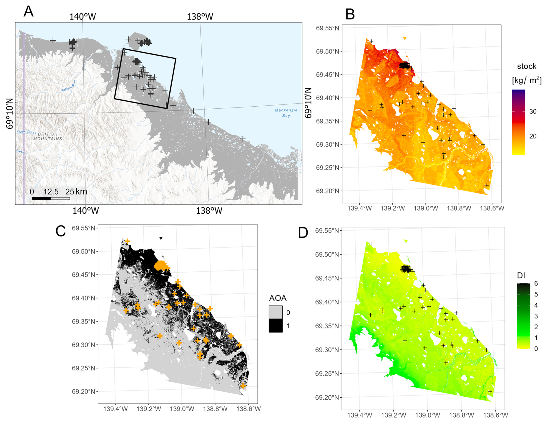
This study focuses on coastal lowland tundra and Herschel Island, the mapping region (Fig. 1A) was selected from the DEM by using areas with an elevation below 180 m. This threshold includes all the area of Herschel Island, while not expanding too far inland where soil data is limited.

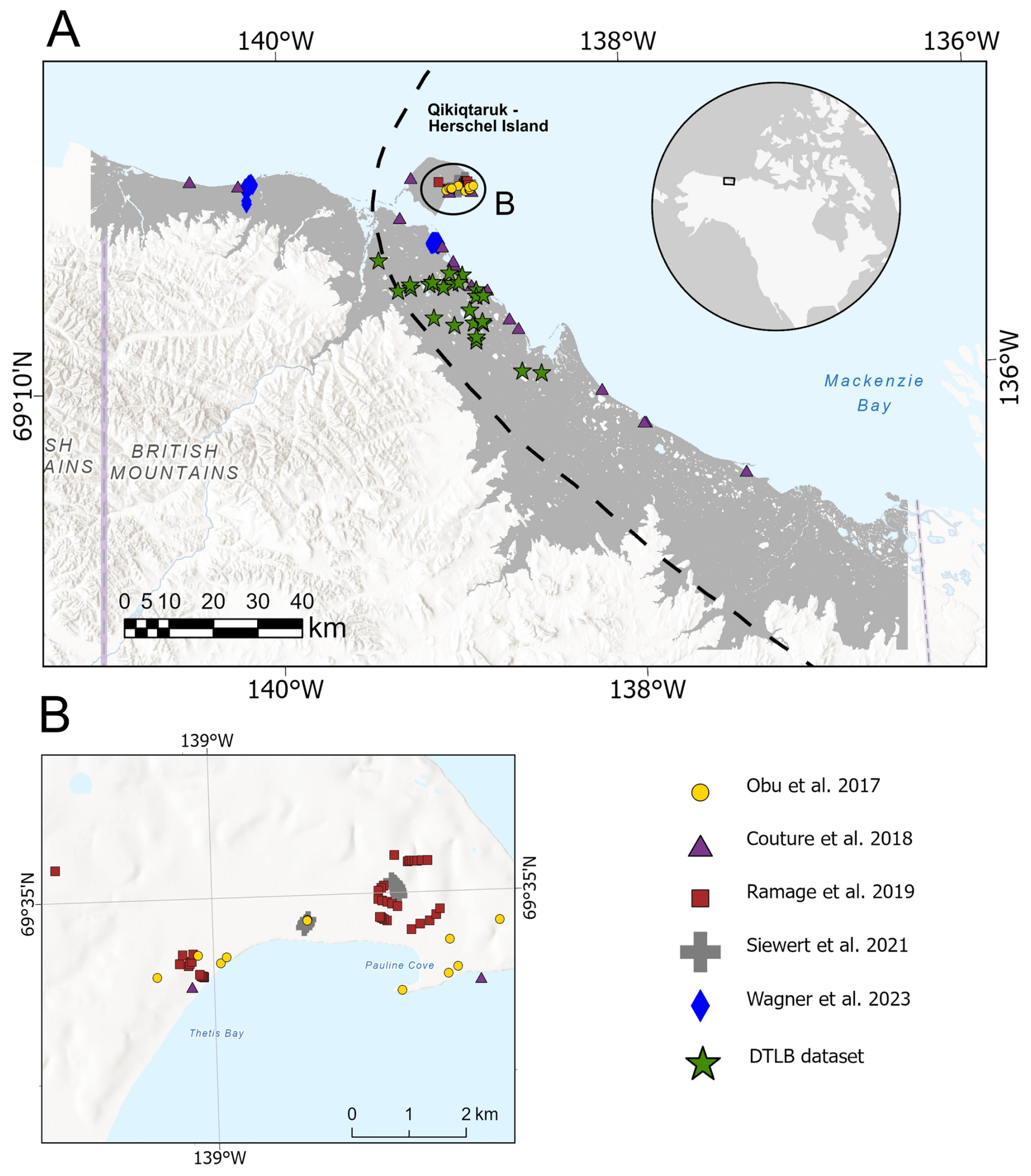
Figure 1 Overview of the study area, locations and sources of the soil data used in this study (A) and zoom-in to the eastern part of Herschel Island (B). The DTLB dataset is a new dataset previously unpublished and included in this study (for more information see Chap. 2.2). The mapping extent is shown in grey on top of the Basemap: ESRI (2024a) | Powered by Esri.

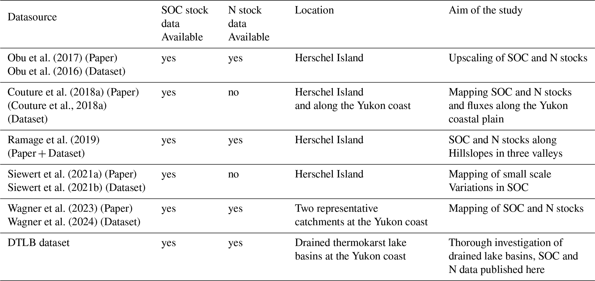
Soil property data were compiled/ combined from multiple published sources (Table 1 and harmonized by converting reported values into the target depth intervals of 0–30 and 30–100 cm using weighted averaging. The laboratory methods differ with some studies using an elemental analyzer (e.g. Elementar vario EL III and Elementar vario MAX C in the study by Obu et al., 2017) or an elemental analyzer (CE Instrument EA 1110 elemental analyzer) coupled to an isotope ratio mass spectrometer (Thermo Fischer Scientific Instruments, Delta V Advantage) (Siewert et al., 2021a) or coupled to a continuous-flow isotopic ratio mass spectrometer (IRMS, DeltaPlus, Finnigan MAT) (Wagner et al., 2023). Further, the timing of the fieldwork differs. Whereas the majority of the studies sampled during the summer (mostly July), the DTLB samples were taken as full frozen cores during spring 2019. These differences in sampling (active layer sampling + coring vs. full frozen coring) have likely affected the results together with the use of different laboratory methods to derive SOC content. We did not account for these differences in the compilation of the dataset. However, permafrost soil research is conducted according to established standardized protocols, facilitating reproducibility and comparability among studies in this region (Ping et al., 2013; Palmtag et al., 2022) which also ensures samples are handled in a similar way. E.g. the coarse fraction >2 mm was excluded from the samples which was mentioned in all studies except by Ramage et al. (2019). The studies were conducted with different sampling designs and goals, causing spatial clustering of data points in the study area. The studies by Siewert et al. (2021a) and Ramage et al. (2019) both followed a transect approach, the study by Obu et al. (2017) sampled representative sites per ecological unit and Couture et al. (2018a) sampled sites along the coast. Wagner et al. (2023) followed a stratified random sampling approach. The study by Siewert et al. (2021a) focuses on soil properties at a small scale and contains values for subpedons which are soil profiles in 10 cm intervals generated from 1 m wide transects. Such a high level of detail was not necessary in our study. Therefore these values were averaged per pedon.

Obu et al. (2017)Obu et al. (2016)Couture et al. (2018a)(Couture et al., 2018a)Ramage et al. (2019)Siewert et al. (2021a)Siewert et al. (2021b)Wagner et al. (2023)Wagner et al. (2024)

Table 1 Overview of the datasets, their sources, aim of the study and availability of SOC and N stock data.

In addition to published data, new data from DTLBs that were sampled during a field campaign in April 2019 was added to this study. The DTLB data covers drained lake basins between Herschel Island and Kay Point at different distances inland from the coast (0.6–14.0 km) and on various elevations (3–65 m), with one central coring location per basin. We cored 24 frozen sediment cores using a SIPRE permafrost corer during this campaign. We aimed to core at least the top metre of sediment including active layer and permafrost and reached 88–200 cm sediment depth, except for core YC19-DTLB-17 (88 cm) and YC19-DTLB-20 (95 cm). All cores were kept frozen until subsampling and analysis. We described core stratigraphies and subsampled all cores at 5 cm resolution or according to stratigraphic boundaries. The stratum of the drainage event was sampled in 2 cm resolution. We weighed the frozen soil samples and measured their dimensions to calculate sample volume. We then calculated water contents as the difference before and after freeze drying, and calculated dry bulk densities as dry sample weight divided by wet sample volume. We analysed freeze dried ground samples for total organic carbon (TOC) content using an Elementar Soli TOC^® cube, and for total nitrogen (TN) content using an Elementar Rapid Max N exceed analyser. All analyses were conducted at laboratories of the Alfred Wegener Institute of Polar and Marine Research in Potsdam, Germany.

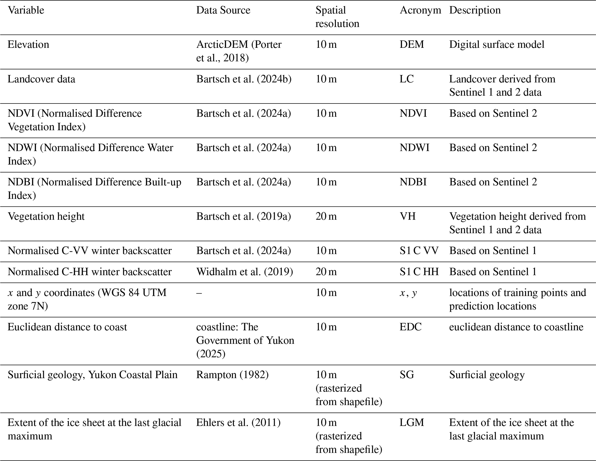
The predictor variables used in the study were taken from published datasets at a spatial resolution of 10–20 m (Table 2). All raster datasets were resampled to 10 m and reprojected to the UTM coordinate system (EPSG code 32607). The landcover data (Bartsch et al., 2019b) was converted into binary variables and the dominating classes in the area were selected. Classes with fewer than 10 sampling points were excluded; these contained between 1 and 7 points, so the cutoff did not omit any reasonably represented classes. The included classes were “dry to moist tundra, partially barren, prostrate shrubs” (LC_class6), “dry tundra, abundant lichen, prostrate shrubs” (LC_class7), “dry to moist tundra, prostrate to low shrubs” (LC_class9), “moist tundra, abundant moss, prostrate to low shrubs” (LC_class10), “moist tundra, abundant moss, dwarf and low shrubs” (LC_class11) and “moist tundra, low shrubs” (LC_class14), . From the surficial geology (Rampton, 1982) classes with at least 10 sampling lications were used, the two classes excluded contained only two or three sampling locations. The included classes were Ff (Alluvial fan), Gp (Outwash plain or valley train), L (Lacustrine plain), Mm (Rolling moraine) and Mr (Ice-thrust moraine ridge).

(Porter et al., 2018)Bartsch et al. (2024b)Bartsch et al. (2024a)Bartsch et al. (2024a)Bartsch et al. (2024a)Bartsch et al. (2019a)Bartsch et al. (2024a)Widhalm et al. (2019)The Government of Yukon (2025)Rampton (1982)Ehlers et al. (2011)

Table 2 Overview of the predictor variables, their sources, spatial resolution, acronym used, and brief description.

2.3 Random forest mapping, area of applicability and uncertainty

This study focuses on creating spatial predictions individually for the mainland and Herschel Island (Fig. 1), creating a separate model that combines all data and comparing the results of the models. All analysis were carried out in R studio using R version 4.1.2 (R Development Core Team, 2021). The random forest algorithm (Liaw and Wiener, 2002) implemented in the package caret (Kuhn, 2008, 2022) was used for mapping SOC and N stocks for the whole area as well as with separate models for Herschel Island and mainland the coastal area. Random forest is a decision-tree based algorithm that builds a large amount of trees based on bootstrap samples of the training data and aggregating their results. This process aims to reduce the prediction error and is also called “bagging” (bootstrap and aggregating). The number of trees (ntree), the amount of covariates selected at each split (mtry) and the minimum amount of training data to continue splitting the tree (nodesize) can be manually defined (Breiman, 1996, 2001).

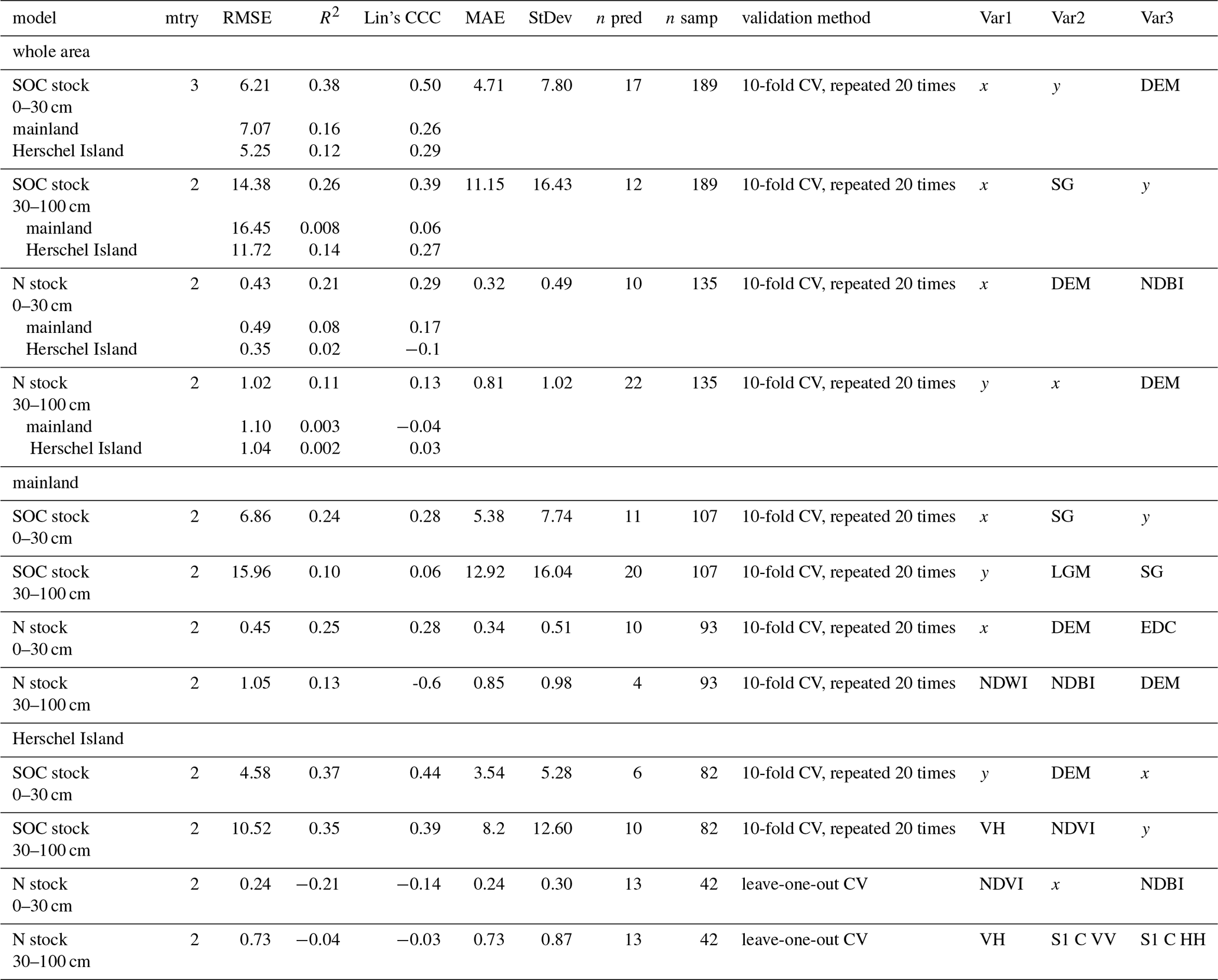
The “boruta” algorithm (Kursa and Rudnicki, 2010) was used for feature selection prior to the training of the random forest models. The algorithm was run with random forest, a maximum repetition of 2500 and a maximum of 1500 trees. The Boruta algorithm serves as a wrapper algorithm and assesses the significance of predictors by contrasting their importance with their corresponding shadows, discarding those with notably lowered importance. These shadows mirror the initial variables, featuring randomly shuffled values while maintaining the original distribution and are regenerated in each iteration. The algorithm stops either as soon as reaching the maximum of specified runs or when only the attributes considered important remain (Kursa and Rudnicki, 2010). Separate random forest models were trained for the depth 0–30 and 30–100 cm for the whole study area including all data. Additional models were trained for Herschel Island and the mainland using the respective data. The reason for creating separate models and predictions was due to Herschel Island being an ice thrust moraine (Rampton, 1982) and therefore geologically very different from the coastal mainland area. The mtry was chosen by grid search where RMSE was the lowest. Mtry is the amount of variables chosen at each split (Liaw and Wiener, 2002). The internal validation was set to 10-fold crossvalidation repeated 20 times for all models, except two where leave-one-out crossvalidation was chosen due to a low amount of datapoints. Ntree was set to 500 and nodesize was kept at its default value of 5. We provide the internal validation results: mtry at which the best performing model was selected according to the lowest RMSE, R² (fraction of %), mean absolute error (MAE), the number of predictors (n pred), the number of samples (n samp) and StDev. We also calculated Lin’s concordance correlation coefficient (CCC) (Lin, 1989) using the package DescTools (Signorell, 2025) because, unlike R² it evaluates both correlation and agreement by accounting for systematic bias, measuring not only how tightly predicted and observed values cluster but also how closely they fall along the 1:1 line of perfect agreement. Additionally, we display for simplicity the first three important variables (short: var) for each model, var1, var2 and var3 (Table 4). From the whole area models we exported predicted values during cross validation and used these to calculate RMSE, R² and Lin's ccc per area (mainland and Herschel Island).

To further evaluate the prediction, the “area of applicability” – method (Meyer and Pebesma, 2021) implemented in the package CAST version 0.9.0 (Meyer et al., 2024) was applied to each model. The area of applicability (AOA) estimates the area where the application of the predicted model is likely accurate and lies within the prediction error (RMSE). The AOA is based on the dissimilarity index (DI) which is calculated based on the minimum distance to the training data within the multidimensional predictor space, where predictors are weighted with respect to their importance in the model prior to the distance calculation. Then a threshold to the DI is applied which is the maximum DI of the training data obtained via crossvalidation resulting in a binary raster layer with 1 representing the AOA and 0 displaying areas outside the AOA. The complete workflow, including all equations, is documented in the Paper by Meyer and Pebesma (2021). In addition to the AOA we used quantile regression forest as described by Yigini et al. (2018) and also applied by Wagner et al. (2023) to estimate the uncertainty which includes the sensitivity of the model to available data and the uncertainty of the model. We applied this workflow to all models.

3 Results

3.1 Data complilation of regional carbon and nitrogen stocks

The individual studies included in this regional study showed a large variety in their distribution of SOC stocks (Fig. 2). Stocks were generally lower on Herschel Island (Fig. 2) compared to the mainland, mirroring geological differences. All the studies carried out solely on Herschel Island showed lower SOC stock values, with the study by Ramage et al. (2019) having the lowest values in the depth increments 0–30 and 30–100 cm with averages of 10.2 and 16.1 kg m⁻² respectively. The study by Siewert et al. (2021a) showed the highest average values with 16.0 and 29.6 kg m⁻² and the study by Obu et al. (2017) was in between with average values of 11.9 and 26.8 kg m⁻². The studies carried out on the mainland showed average values of 17.6 and 31.2 kg m⁻² (DTLB dataset) and 21.5 and 42.6 kg m⁻² (Wagner et al., 2023). The study by Couture et al. (2018b) used sites on Herschel Island as well as coastal sites on the mainland, however average values were similar when separating the values for Herschel Island and the mainland (Table 3).

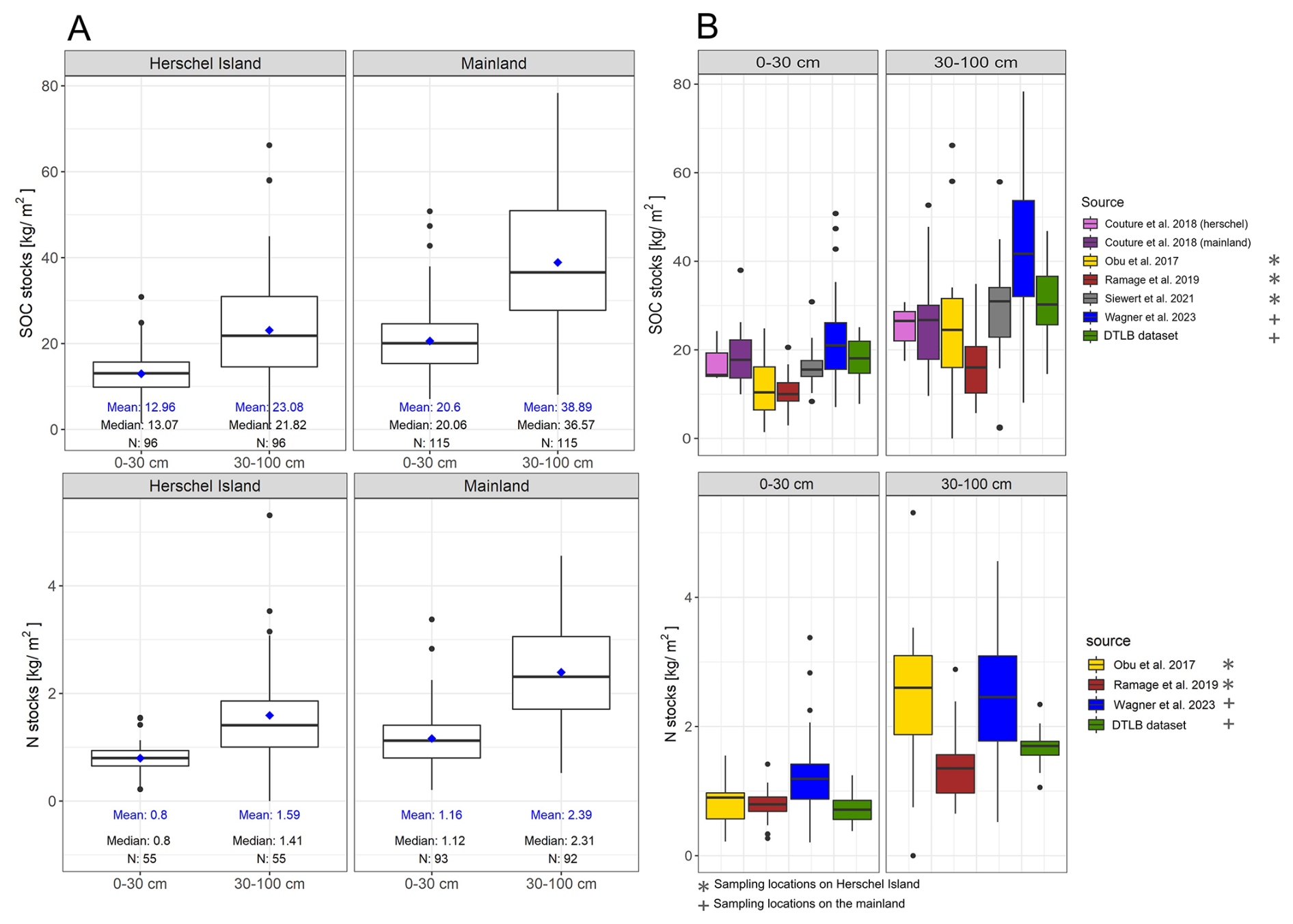
Figure 2 Soil organic carbon (SOC) and nitrogen (N) stocks per depth interval separated into mainland and Herschel Island (A) and per study area (B).

Table 3 Mean, median, standard deviation (StDev) and number of datapoints per study used in this study. (The Dataset by Couture et al. (2018) consists of sites from Herschel Island and the mainland and the values are therefore presented for the whole dataset and split per site). NA = not available.

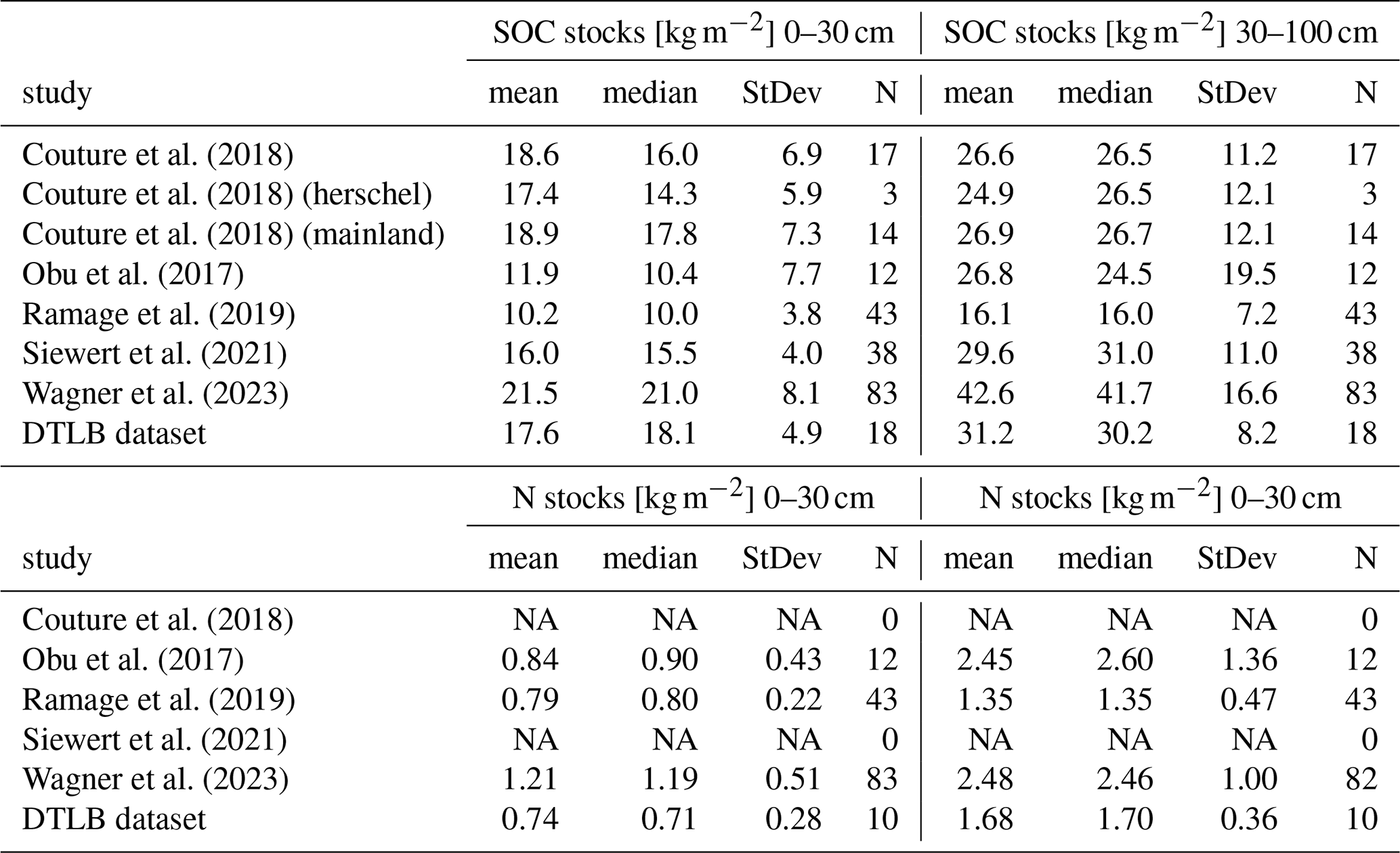
Table 4 Results of the random forest models. The table shows the internal validation results: mtry at which the best performing model was selected according to the lowest RMSE. R² (fraction of %), Lin's CCC, mean absolute error (MAE), the number of predictors (n pred), the number of samples (n samp) and StDev are displayed together with the first three important variables for each model (Var1, Var2 and Var3). Additionally the predictions during crossvalidation for the whole area models were saved and RMSE, R² and Lin's CCC were calculated for the areas mainland and Herschel Island. The table continues on the next page.

In contrast, N stocks showed a different pattern with higher N stocks at the sites of the studies by Obu et al. (2017) and Wagner et al. (2023), especially in the depth 30–100 cm compared to the datasets by Ramage et al. (2019) and the DTLB dataset (Fig. 2 and Table 3). After dividing SOC and N values between “mainland” and “Herschel Island”, average SOC stock values were 13.0 kg m⁻² in depth 0–30 cm and 23.1 kg m⁻² at 30–100 cm for Herschel Island and 20.6, while average SOC stock values for the mainland were 38.9 kg m⁻². The N stocks on Herschel Island were 0.8 and 1.59 and 1.16 and 2.39 kg m⁻² on the mainland (Fig. 2). The distribution further shows that mean and median values are close (Fig. 2).

3.2 Random Forest mapping and model validation assessment

The models for the whole area have R² values of 0.38 and 0.26 for the SOC stocks and 0.21 and 0.11 for the N stocks (Table 4). When separating the accuracy measures from the whole area models into the data for the mainland and Herschel Island R² values are lower with for example 0.16 and 0.12 for the SOC stocks at 0–30 cm depth and 0.008 and 0.14 for 30–100 cm depth. The separate models for the mainland had R² values of 0.24 and 0.10 for the SOC stocks at 0–30 and 30–100 cm. The models for the SOC stocks at Herschel Island had an R² value of 0.37 for 0–30 cm and 0.35 for 30–100 cm. The RMSE values of most models were below the standard deviation (StDev) of the distribution of the data values. Most of Lin's ccc values are higher than the R² of the respective models (Table 4). The models for SOC stocks often performed better regarding R² and Lin's ccc values. Comparing upper soil 0–30 cm vs. lower soil 30–100 cm, the models for the upper soil performed better (Table 4). The highest values for SOC and N stocks are predicted in the west of the study area and areas close to the coast with lower values with increasing distance from the coast (Fig. 3). The average SOC stocks (Table 5) for the models using all data for the whole area were 17.2 kg m⁻² at 0–30 cm and 31.5 kg m⁻² at 30–100 cm depth. The N stocks were 0.93 and 2.11 kg m⁻² respectively. When both SOC and N stocks, were modelled separately for Herschel Island and the mainland, higher SOC and N stocks were modelled on the mainland and lower SOC and N stocks on Herschel Island. SOC stocks at 0–30 cm depth were 18.9 kg m⁻² for the mainland and 12.8 kg m⁻² for Herschel Island, when both areas were modelled separately, in contrast to using the all data for the whole area, which resulted in an average of 17.2 kg m⁻² (Table 5).

Figure 3 Prediction of soil organic carbon (SOC) and nitrogen (N) stocks for the whole study area using all data (Basemap: ESRI (2024b) | Powered by Esri).

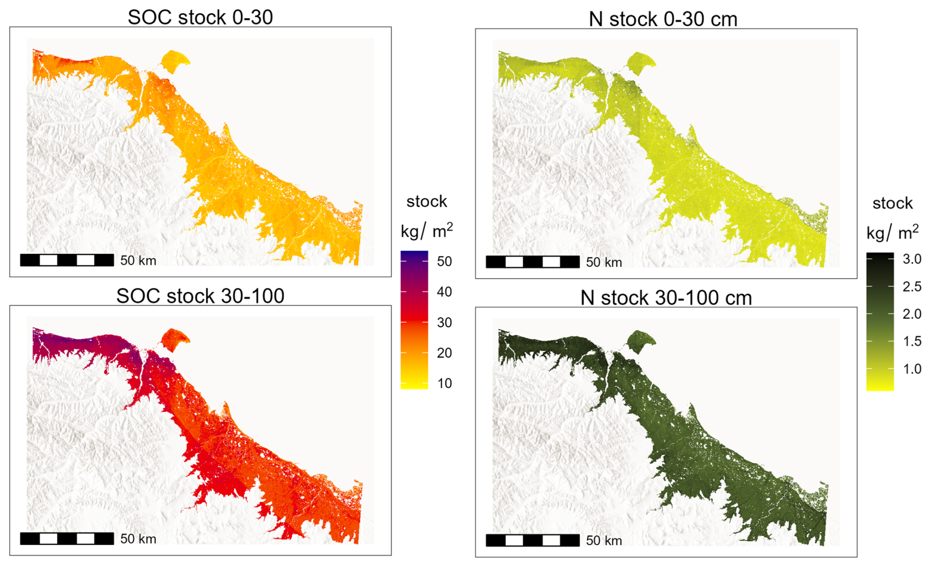
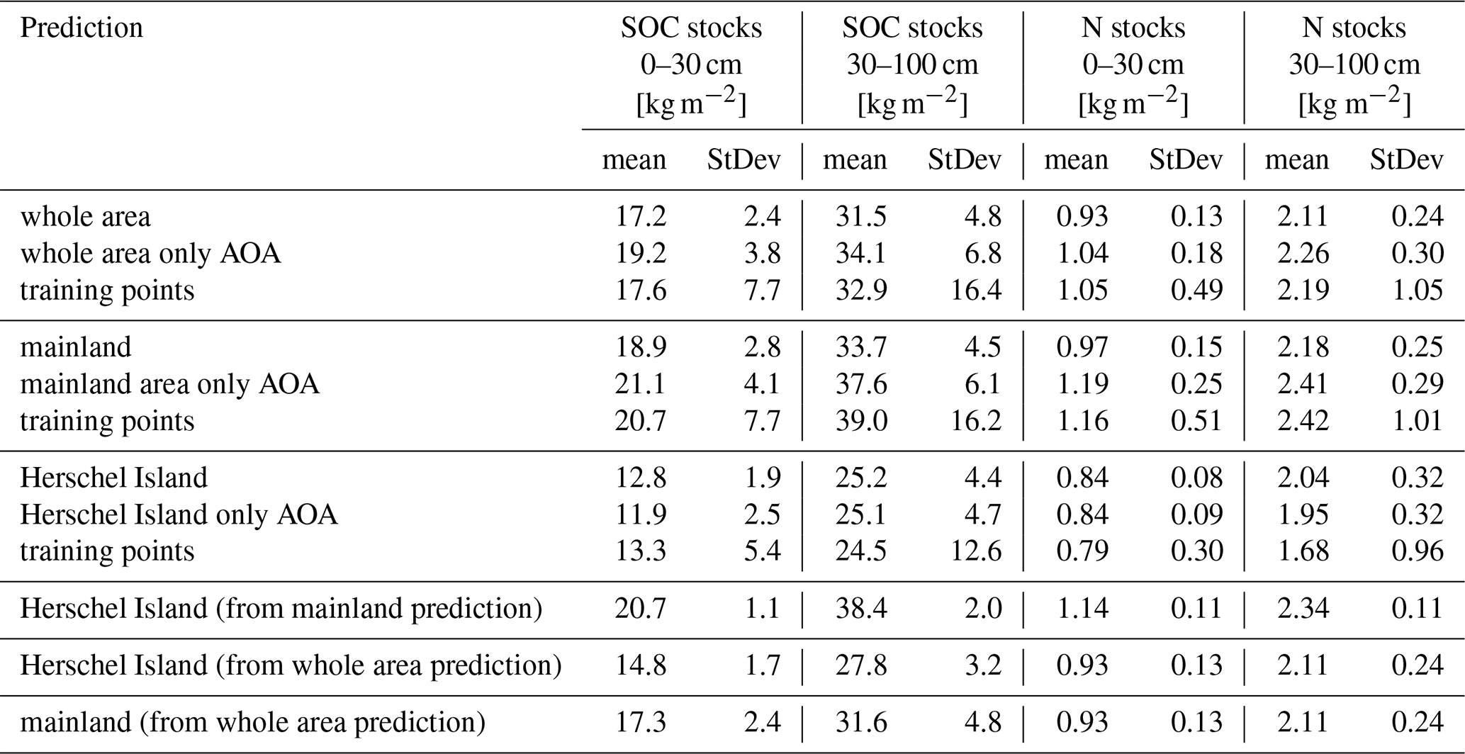
Table 5 Comparison of average soil organic carbon (SOC) and nitrogen (N) stocks for each model prediction depicting the whole area and additionally the AOA of each respective prediction and predictive model (For more descriptive statistic values see Table S2). The average SOC and N stock values from the training points is added to the table for context.

The x and y coordinates and the elevation were among the most important predictor variables across the majority of the models (Table 4, Fig. 4). While Fig. 4 shows examples of two variable importance plots, the variable importance for the remaining models is shown by Figs. S1 and S2 in the Supplement. The most important variables for the whole area models are mainly the geographic location represented by the x and y coordinates and the geology. For the mainland models the geographic location, elevation, geology and the LGM extent were among the most important variables. In contrast, for the Herschel Island models the geographic location was important in the depth 0–30 cm but not on the depth 30–100 cm. Here variables such as vegetation height, NDVI and radar backscatter were important.

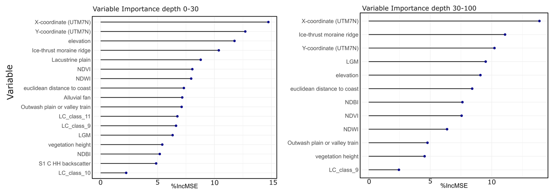
Figure 4 Variable importance for the models predicting soil organic carbon (SOC) for the whole area in depth 0–30 and 30–100 cm. For the variable importance for all models see supplement. (variables: DEM = digital elevation model, NDVI = Normalised Difference Vegetation Index, NDWI = Normalised Difference Water Index, NDBI = Normalised Difference Built-up Index, vegetation height, LC_class9 = dry to moist tundra, prostrate to low shrubs, LC_class10 = moist tundra, abundant moss, prostrate to low shrubs, LC_class11 = moist tundra, abundant moss, dwarf and low shrubs, S1 C VV backscatter = Normalised C-VV winter backscatter from Sentinel-1, S1 C HH backscatter = Normalised C-HH winter backscatter from Sentinel-1), ice-thrust moraine ridge, Lacustrine plain, Alluvial fan, and Outwash plain or valley train = Surficial Geology classes, LGM = ice sheet extent at the last glacial maximum.

3.3 Area of Applicability (AOA) and uncertainty with quantile regression forest

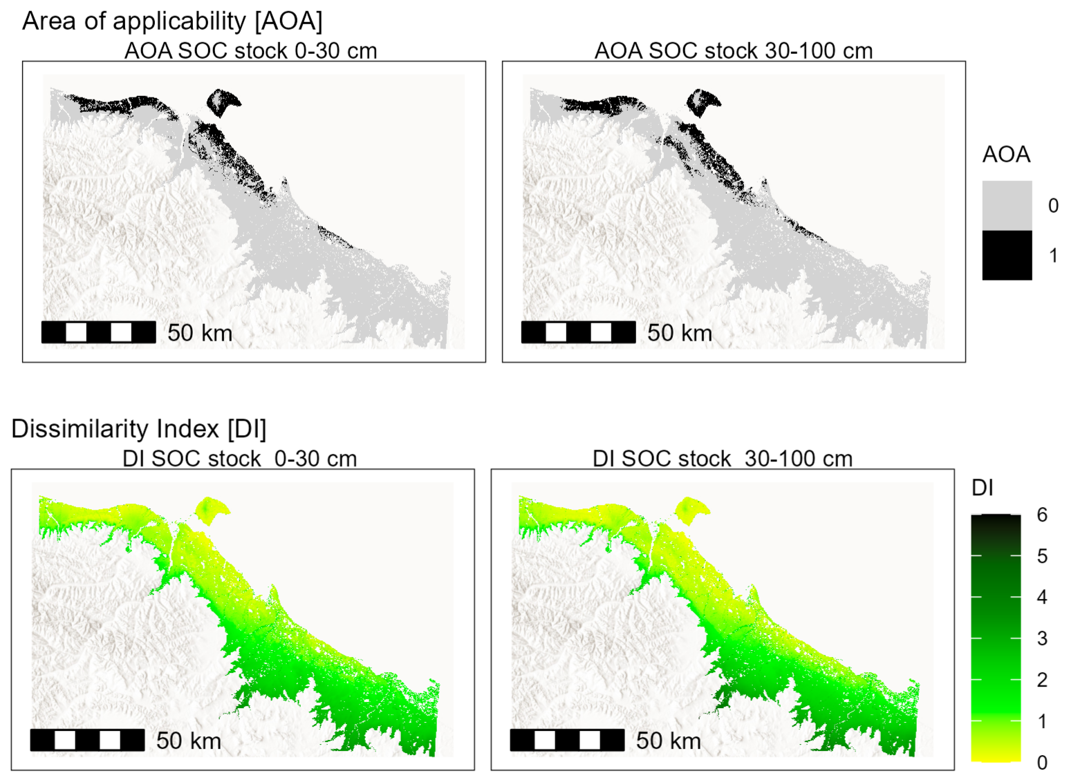
The analysis of the DI and AOA showed that areas where models were not reliable are mostly located around streams and lakes, as well as higher elevation areas further away from the coast (Figs. 5 and 6). The analysis also shows that large areas where no samples are available, had a high DI, limiting the applicability of the model. Generally, areas that are too different from the sampled areas had a high DI and are outside the AOA. However, sites with similar sample-predictor relations to the sampled sites, but further away, were still suitable and within the AOA (Fig. 6). The general patterns show that the applicable area was defined within close vicinity to the sampling locations (Fig. 6). In models using all data and the models for the mainland, predicted SOC and N stock values inside the AOA were generally higher (for example 21.1 ± 4.1 kg C m⁻² inside the AOA compared to 18.9 ± 2.8 kg C m⁻² for the mainland model at 0–30 cm depth; Table 5). For Herschel Island there was no difference between AOA and whole area for the N stock models and and slight differences for the SOC stock models (Table 5).

The results of the quantile regression forest uncertainty (Figs. S5, S6 and S7) showed areas around lakes and streams and areas further away from the sampling locations as having high uncertainty, similar to the AOA analyses. At Herschel Island (Fig. S7) the highest uncertainty is towards the coast, in depressions and near streams. The area on Herschel Island, that has been identified as applicable by the AOA method, has no visible higher uncertainty measured by the quantile regression forest method than the inapplicable area.

Figure 5 Area of applicability (AOA) and dissimilarity index (DI) for the predictive model of SOC stocks for the whole area. For DI thresholds that determine AOA see Table S1 (Basemap: ESRI (2024b) | Powered by Esri).

Figure 6 Zoom-in to an area (A, black square) with SOC stock distribution for depth 0–30 cm (B) the respective area of applicability (C) and dissimilarity index (DI). The datapoints are shown with cross symbols (Basemap in A: ESRI (2024a) | Powered by Esri).

4 Discussion

This study provides the most comprehensive compilation of SOC and N data available for the region to date. This dataset serves as a benchmark for future studies, while also highlighting the substantial uncertainties that remain due to limitations in spatial coverage and data distribution.

4.1 Regional soil carbon and nitrogen data reveal heterogeneity with implications for modeling

Our study shows that already at a regional level there is a very high heterogeneity in field data, challenging the predictive ability of models. The full range of the available data in regional, but also in pan-Arctic synthesis must be representative for the entire study area. Data collection and sampling strategies from local studies are often tailored to specific research questions. As a result, some landscape features may be overrepresented while others are underrepresented in the available data, potentially limiting the ability to capture spatial variability in regional analyses. To address this, it is important to evaluate the distribution of the target variable at the sampling locations in the context of the broader landscape. The Area of Applicability (AoA) method provides a way to do this by comparing the feature space of the covariates at sampled sites to the feature space across the entire study area. Areas where the covariate space is not covered by existing samples can be excluded from regional predictions and can also inform the planning of future sampling campaigns to better capture landscape heterogeneity. Since the AoA method evaluates only the feature space of the covariates and does not provide uncertainty estimates, complementary approaches, such as quantile regression forests, are essential for quantifying uncertainty in random forest predictions.

The data shows that SOC and N stocks are lower at Herschel Island than at the mainland (Fig. 2). This is likely due to Herschel Island being an ice thrust moraine (Rampton, 1982) and therefore being geologically different to the mainland. When looking at the studies individually, large differences occur even when comparing the studies only carried out on Herschel Island (Fig. 2). This is attributed to the different aims of the studies and site selection. While Obu et al. (2017) covered representative sites for different ecological units on Herschel Island, Ramage et al. (2019) sampled hillslopes in three valleys which show significant levels of erosion. Erosive relocation of organic material which explains why SOC and N stocks are lower compared to the other studies. Siewert et al. (2021a) sampled representative sites in three typical ecological units on Herschel Island: hummocky tussock tundra, non-sorted circle tundra and IWP tundra. The selective sampling of specific representative areas was to study multi-scale variation of SOC distribution in specific permafrost landforms. The sites did not undergo significant erosion/ degradation and therefore SOC stocks are higher than at the sites of Ramage et al. (2019) and slightly higher than Obu et al. (2017). The latter covers also moderately and strongly disturbed sites which show lower amounts of SOC are found in the upper soil (0–30 cm) as well as in the whole profile of 1 m. Wagner et al. (2023) studied two typical small coastal catchments with dense sampling density. Particularly the sampling sites at Ptarmigan Bay were located in areas of high organic layer thickness (Rampton, 1982). The DTLB samples were exclusively from organic rich deposits (peat above lake sediment).

4.2 Modeling and mapping SOC and N stocks: model and prediction results in the context of their limitations and methodological challenges

Our analysis highlights the challenge of scaling from local (pedon) to regional study areas. At the pedon scale, permafrost soils are highly heterogeneous (Siewert et al., 2021a) and this variability is still evident at coarser spatial scales. The models for the entire area explain only a small fraction of spatial heterogeneity in SOC and N stocks (R² for SOC stock 0–30 cm: 0.38, 30–100 cm: 0.26; R² for N stock 0–30 cm: 0.21, 30–100 cm: 0.11, Table 4). Partitioned per study area the R² values show that the models perform worse than the respective individually trained models for the mainland and Herschel Island. For example the SOC stocks for 0–30 cm depth have R² values of 0.16 and 0.12 for the mainland and Herschel Island respectively while the individual models have 0.24 and 0.37. This indicates that individually trained models might handle the local variability better. The models for Herschel Island show higher R² values for SOC (0.37 and 0.35), which could be due to a combination of factors: (1) lower natural soil variability on Herschel Island, (2) better representation of the soil data, or (3) stronger relationships between the predictors and SOC at this site. For all models Lin's ccc values were higher than R². This indicates that agreement between predicted and observed values is stronger than indicated by correlation alone, despite the limited model performance. We therefore recommend that users of these maps carefully consider which dataset to use: the full-area predictions provide a consistent regional overview, whereas the individually trained models may better capture local variability and could be more appropriate for studies focused on specific subregions.

For Herschel Island, there was a higher data density (0.8 samples per km²; n=78 for SOC, area approximately 108 km²) than on the mainland (0.02 samples per km²; n=107 for SOC stocks, area approximately 4465 km²). This has likely affected the accuracy of the models and may explain why mainland models have a lower R² values. It is also possible that the exact data density is less important than the spread and representation of the data in relation to natural variability between landscape types. Several of the studies on Herschel Island included representative sampling of multiple ecological units on the island, ensuring a range of landscape types are well characterised by the data. Models for SOC stocks also outperform those for N stocks, likely reflecting the smaller number of sites with N data available, as several locations only report SOC measurements.

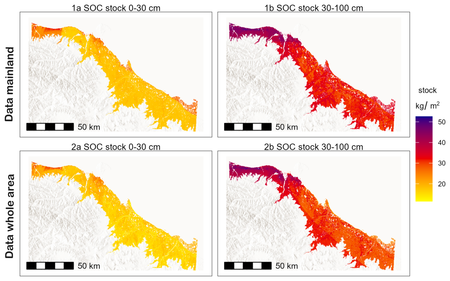
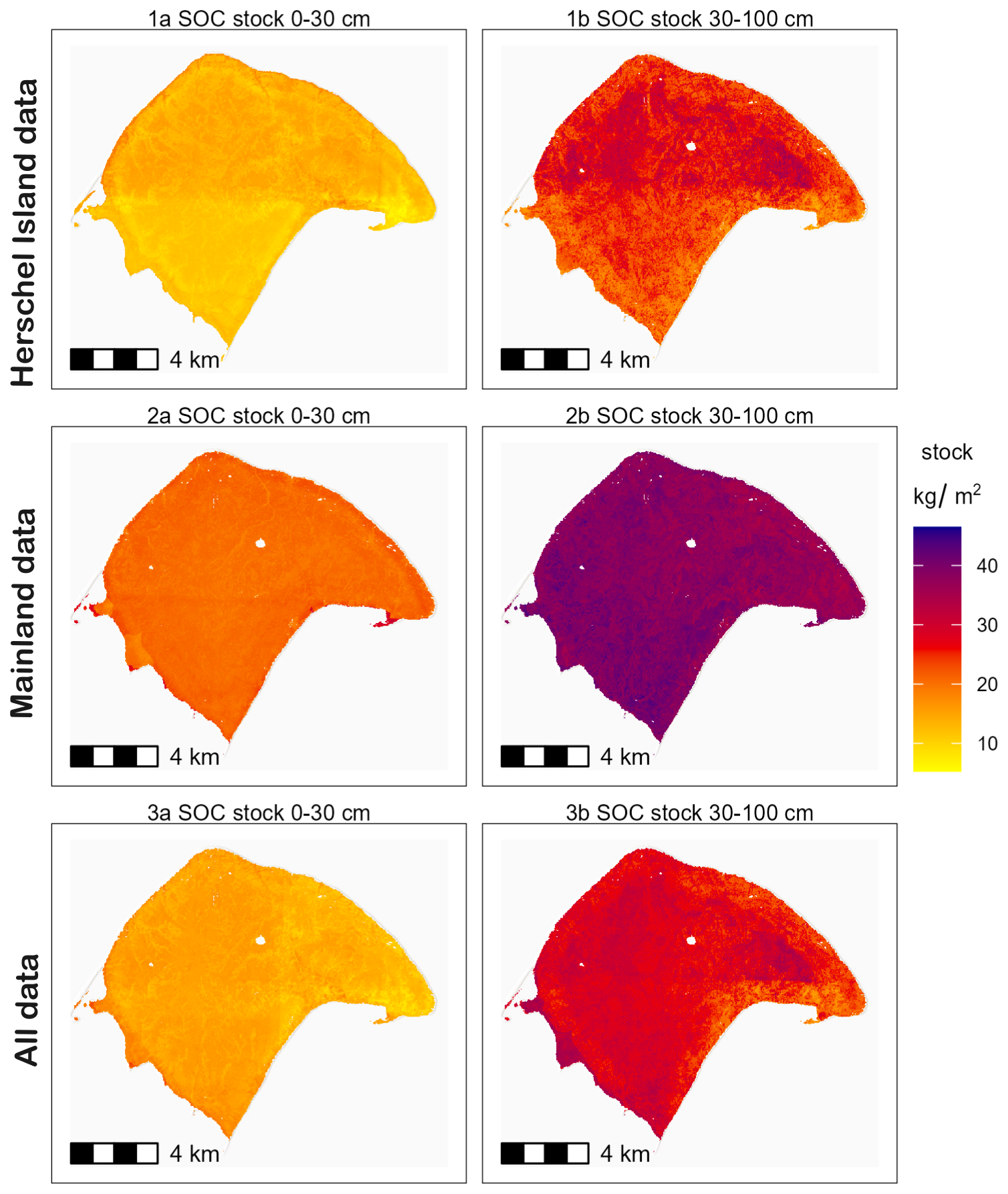
The strong local heterogeneity in SOC and N stocks makes model predictions highly sensitive to the spatial origin of the training data. Including or excluding data from geologically distinct subregions, such as the geologically different Herschel Island compared to the mainland, can substantially alter predicted patterns and underscores the uncertainty of extrapolating beyond the training domain. Figure 7 displays the SOC stock distribution for the mainland area when using only training data from the mainland (Fig. 7(1a) and Fig. 1(1b)), in contrast to training a model that also includes data from Herschel Island (Fig. 7(2a) and (2b)). When using all data, including Herschel Island, SOC stocks are lower, with averages of 17.0 and 31.6 kg C m⁻² for 0–30 and 30–100 cm depth, respectively. This is in large contrast to using only data derived from the mainland where SOC stocks are considerably higher, with 18.9 and 33.7 kg C m⁻². An opposing pattern is displayed in Fig. 8, where using all data results in higher SOC stocks at Herschel Island in comparison to using Herschel Island data only. The map with the largest SOC stocks is produced when interpolating from mainland data to Herschel Island (Fig. 8(2a) and (2b)).

Figure 7 Comparison of soil organic carbon (SOC) stock for the coastal mainland region using only the mainland data (1a, 1b) and using all data (2a, 2b) (Basemap: ESRI (2024b) | Powered by Esri).

Figure 8 Comparison of soil organic carbon (SOC) stocks at Herschel Island using only datapoints on Herschel Island (1a, 1b), predicting (extrapolating) SOC only based on data from the mainland (2a, 2b) and using da for the entire area (3a, 3b) (Basemap: ESRI (2024b) | Powered by Esri).

This analysis of the sensitivity of model predictions to the spatial origin of training data highlights that careful data selection is crucial for studies at a regional scale. Data representation and potential site biases are also likely to be important for pan-Arctic SOC and N assessments. Mishra et al. (2021) carried out spatial predictions for three regions separately: the North American, the Eurasian and the Tibetan Permafrost region. Our study shows that differences in SOC stocks are significant even when comparing adjacent local scale areas. As the exclusion or inclusion of certain data has the potential to significantly influence SOC and N stock predictions, a more detailed differentiation, e.g. through geological units or terrain characteristics, would be recommended. Herschel Island in comparison to the mainland, especially the area in close proximity, is particularly interesting, since soil forming factors such as landscape age, climate and vegetation are very similar, however the parent material differs. The area at Ptarmigan Bay consists mostly of glaciofluvial and rolling moraine deposits (Rampton, 1982). In contrast Herschel Island consists of massive ground ice later buried by marine sediments (Burn, 2012). These differences in parent material offer different conditions for soil development as their texture and geochemical composition differ. Studies show that carbon enrichment through cryoturbation differs with grain size leading to higher carbon enrichment in higher coarse silt to very fine sand fractions (Palmtag and Kuhry, 2018).

An assessment of uncertainty and model representation is crucial in digital soil mapping. Hugelius et al. (2014) used upscaling of SOC stocks based on thematic maps representing the physiography and provide an uncertainty assessment in their study that includes a “representation error” in the regions with lower data density. Similar considerations should be incorporated in pan-Arctic studies that use DSM approaches such as machine learning models. The data used in synthesis studies might be highly clustered and can show a high variability on regional and local level. This phenomenon is discussed by Meyer and Pebesma (2022), mentioning that geographic clusters of the data do not necessarily mean gaps in the feature space, i.e. the sample – predictor relationships may still represent the entire area.

To assess whether the presented models of our study are applicable for the total study area, we used the AOA method (Meyer and Pebesma, 2021). It is expected that the dry areas of riverbeds and areas around lakes on the mainland are excluded after applying the AOA, because these areas do not contain any sampling sites. Areas with larger distance from the coast were not extensively sampled and therefore DI rises with distance from the coast. The average SOC and N stocks were slightly higher compared to the initial prediction when excluding not applicable areas. This shows that the predictions outside the AOA are at the lower end of the spectrum of predicted values (Table 5). We believe that values that are not represented by AOA are more likely to be underpredicted than overpredicted when using random forest for our study area.

The AOA method focuses on the relationship between covariates and data. We also applied the quantile regression forest to the mainland and Herschel Island models for SOC stocks to assess uncertainty. This method estimates uncertainty from two sources: the model itself and variations in the data. Data uncertainty is assessed by repeatedly applying a random forest model to different datasets, while model uncertainty is calculated using quantile regression forests, and both are combined into a final uncertainty map (Yigini et al., 2018). For all models there is no clear trend whether a high uncertainty could correlate with a high dissimilarity index (Fig. S8). The quantile regression forest method focuses on the uncertainty on a pixel basis. Multiple model runs are used to assess the sensitivity of the model to available data and quantile regression forest is used to calculate a probability distribution for the values each pixel can take on. In contrast, the AOA method assesses the applicability based on a certain model and the importance of the variables. To best assess the accuracy of the predictions, we recommend using not exclusively one of the two methods.

The selection of the covariates also significantly impacts the prediction power of models. Many studies in digital soil mapping in general (e.g. Hengl et al., 2017) but also pan-Arctic studies (Mishra et al., 2021) include parameters derived from digital elevation models such as slope, curvature, aspect, flow direction, flow accumulation, etc. Coastal lowland tundra areas generally have very flat terrain and are close to sea level, which are critical aspects when considering the use of topographic derivates. Parameters such as flow direction and flow accumulation may not represent the complexity of flow patterns in IWP terrain (e.g. Speetjens et al., 2024). Most models for the whole area and the mainland consider the geographic location, the geology and elevation among the most important variables, reflecting broad-scale spatial patterns, the influence of substrate and soil-forming materials on carbon and nitrogen content, and gradients in temperature, moisture, and drainage that affect soil properties. On Herschel Island, local vegetation characteristics and surface properties such as vegetation height, NDVI and radar backscatter are important predictors of SOC and N stocks, likely reflecting the relatively uniform geology of the island and the greater influence of fine-scale surface indicators compared to broad-scale spatial variables.

A major limitation of our study is the low explanatory power of the models as indicated by the low R² and Lin's ccc values explaning only up to half of the spatial variability. in SOC and N stocks. This suggest that to achieve high predictive power across this region, systematic additional soil sampling in addition to the compilation of local studies would be needed. A dataset that represents all landscape types, and predictors that co-vary with soil variability across space are needed. Lastly, a quantification of errors in the dataset spanning from differences of point in time of sampling, sampling errors, differences between devices measuring SOC and N were not quantified and outside the scope of this study.

4.3 Comparing local scale results to regional scale synthesis

By integrating all available SOC and N data for the region, this study establishes a benchmark dataset, representing the most comprehensive regional-scale assessment currently possible. Substantial uncertainties remain, stemming from the uneven spatial distribution of sampling points and the inherent challenges of collecting soil data in remote permafrost landscapes. Previous studies in the region often rely on class-based averages with limited region-specific observations, or, in the case of digital soil mapping, coarser-resolution datasets. Here we present our findings in the context of existing local and regional data, emphasizing that our compilation, which incorporates both published and previously unpublished observations, provides an enhanced regional perspective while acknowledging its limitations.

The two mainland sites Ptarmigan Bay and Komakuk Beach were studied on a high spatial resolution (2 m) (Wagner et al., 2023) and SOC stocks were 40 and 66.6 kg C m⁻² respectively. The results of our study show 63.7 and 59.7 kg C m⁻² respectively with the entire area models and 64.3 and 62.1 kg C m⁻² with the mainland only models. For Ptarmigan Bay, (Hugelius et al., 2013) suggest 92.8 kg C m⁻² and (Mishra and Gautam, 2022) 63.4 kg C m⁻². At Komakuk Beach, (Hugelius et al., 2013) estimated 18.1 kg C m⁻². Furthermore, this study shows that there are high local differences between different geographic areas when comparing different individual high resolution studies. In contrast, the results of the regional mapping lead to similar results for Komakuk Beach and Ptarmigan Bay. However, the SOC stocks for Komakuk Beach using the model with all data is lower than using the mainland only model. This could be partially explained by the inclusion of data from Herschel Island. Our study included more samples than Obu et al. (2017) and our methods differ (machine learning in contrast to class matching), leading to different average SOC stocks when comparing both studies. Obu et al. (2017) show 34.8 kg C m⁻² for the upper metre of soil while our results show 38.0 kg C m⁻² with the Herschel Island models (Table S3). Large scale studies seemed to overpredict SOC stocks at Herschel Island. The estimated SOC stocks in the upper metre are according to Hugelius et al. (2013) 55.3 kg C m⁻² at Herschel Island and 58.6 kg C m⁻² according to Mishra and Gautam (2022). For the mainland, Hugelius et al. (2013) provide an average of 64.5 kg C m⁻² and Mishra and Gautam (2022) 52.8 kg C m⁻², though the latter does not account for the whole mainland area due to data gaps. Our study shows 52.5 kg C m⁻² for the mainland, which lies in between the studies mentioned above (Table S3).

Our study provides the most up-to-date and comprehensive assessment of soil C and N stocks for the region. Our results highlight that geological and landscape differences within the region play a key role in SOC and N distribution, emphasizing the need to consider these factors in regional-scale analyses and future sampling strategies. The dataset by Mishra and Gautam (2022) has a data gap at Komakuk Beach, west of Komakuk Beach and for a large portion of the area where DTLBs were sampled. This shows that the coastal area lacks accurate maps of SOC stocks. Hence, our study contributes in complementing existing studies and provides moderate resolution datasets at regional scale. Furthermore, the fact that local SOC stocks can vary widely between studies needs to be taken into account in future carbon budget studies.

5 Conclusion

Our study combines existing soil data from different studies that have been carried out at the Yukon coastal plain, providing an estimation of regional SOC and N stocks at 10 m spatial resolution for the top metre of soil. Furthermore, our study complements pan-Arctic estimates, especially as coastal areas are not well represented and there are large data gaps in pan-Arctic datasets. The average SOC stock for the upper metre for the entire area is 48.7 ± 6.6 kg m⁻² and the N stock 3.03 ± 0.30 kg m⁻². Separate models provide for Herschel Island the values of 38.0 ± 5.6 kg C m⁻² and 2.87 ± 0.34 kg N m⁻² respectively, at the mainland 52.2 ± 6.3 kg C m⁻² and 3.15 ± 0.32 kg N m⁻². Users should select the model according to the intended scale: the whole area model for regional assessments, and the separate models for site-specific applications.

Our study leads to several recommendations. First, we want to highlight that the usage/exclusion of data might lead to very different model results, especially when extrapolating to areas with differences in geological genesis or soil parent material composition. We therefore recommend that pan-Arctic studies not only subdivide data into geographic regions, but also following landscape history. Second, we recommend the usage of the AOA to assess whether the relation between covariates and target variable is represented across the whole study area, as this approach can also help to determine new sampling sites. This requires additional spatial regional datasets that can be used as covariates that represent the soil forming factors. Third, we recommend using quantile regression forest to estimate the model uncertainty. Overall, we conclude that multi-scale studies are needed for better predictions of global soil C budgets in the wake of climate change, because they can provide a potent bridge between high resolution local studies and moderate resolution pan-Arctic studies. This paper highlights challenges in combining data from existing studies for DSM applications, which should be considered in future research. The use of existing datasets can substantially reduce costs, yet challenges due to e.g. spatial clustering of the data remain. Our findings can inform the design of future sampling campaigns in remote permafrost regions, aiming to maximize efficiency while minimizing expenses.