Mapping near-real-time soil moisture dynamics over Tasmania with transfer learning

Soil moisture, an essential parameter for hydroclimatic studies, exhibits considerable spatial and temporal variability, which complicates its mapping at high spatiotemporal resolutions. Although current remote sensing products offer global estimates of soil moisture at fine temporal resolutions, they do so at a coarse spatial resolution. Deep learning (DL) techniques have recently been employed to produce high-resolution maps of various soil properties; however, these methods require substantial training data. This study sought to map daily soil moisture across Tasmania, Australia, at an 80 m resolution using a limited set of training data. We assessed three modeling strategies: DL models calibrated using an Australian dataset (51 411 observation points), models calibrated using the Tasmanian dataset (9825 observation points), and a transfer learning technique that transferred information from the Australian models to Tasmania using region-specific data. We also evaluated two DL approaches, i.e., multilayer perceptron (MLP) and long short-term memory (LSTM). The models included the Soil Moisture Active Passive (SMAP) dataset, weather data, an elevation map, land cover, and multilevel soil property maps as inputs to generate soil moisture at the surface (0–30 cm) and subsurface (30–60 cm) layers. Results showed that (1) models calibrated from the Australian dataset performed worse than Tasmanian models regardless of the type of DL approaches; (2) Tasmanian models, calibrated solely using local data, resulted in shortcomings in predicting soil moisture; and (3) transfer learning exhibited remarkable performance improvements (error reductions of up to 45 % and a 50 % increase in correlation) and resolved the drawbacks of the two previous models. The LSTM models with transfer learning had the highest overall performance with an average mean absolute error (MAE) of 0.07 m³ m⁻³ and a correlation coefficient (r) of 0.77 across stations for the surface layer as well as $\text{MAE}=\mathrm{0.07}{\mathrm{m}}^{\mathrm{3}}{\mathrm{m}}^{-\mathrm{3}}$ and r=0.69 for the subsurface layer. The fine-resolution soil moisture maps captured the detailed landscape variation as well as temporal variation according to four distinct seasons in Tasmania. The models were then applied to generate daily soil moisture maps of Tasmania, integrated into a near-real-time monitoring system to assist agricultural decision-making.

1 Introduction

Soil moisture plays an essential role in land surface modeling, serving as a key link between soil, climate, and vegetation. In hydrology, it is frequently used as a proxy for evaluating hydrological extremes, including drought assessment (Taufik et al., 2022; Lin et al., 2023). In agricultural practices, soil moisture provides valuable information for soil water management and crop yield predictions (Yang et al., 2021). Mapping and monitoring soil moisture present significant challenges for soil scientists due to its high spatial and temporal diversity. The variation in soil moisture is influenced by factors such as climate, topographic features, vegetation cover, and soil characteristics, including clay content, soil aggregation, and organic carbon content (Minasny and McBratney, 2003; Védère et al., 2022).

Globally, soil moisture information is available in various formats and with various coverage. At the point scale, the International Soil Moisture Network provides a harmonized measured soil moisture database worldwide (Dorigo et al., 2021). In Australia, soil moisture observations can be found in the OzNet and OzFlux databases (Smith et al., 2012; Beringer et al., 2016). However, despite accurate information on observations at the point level, the spatial coverage of these measurements is limited, meaning that soil moisture content in unmonitored areas is uncertain. To bridge this gap, various spatial datasets were generated to complement the point-scale measurements. Remote sensing, geostatistical models, water balance models, or a combination of them are the principal methods to derive soil moisture images covering multiple scales of space and time.

Notable soil moisture sources across the Australian continent include the Australian Water Resource Assessment Landscape (AWRA-L), which provides a 5 km resolution soil moisture level based on the water balance approach (Frost et al., 2016). Using the OzFlux and OzNet data points as input, this dataset covers moisture prediction for three soil layers (0–10, 10–100, and 100–600 cm). The Soil Moisture Integration and Prediction System (SMIPS) provides a daily soil water balance map at 1 km resolution by integrating machine learning and water balance models (Wimalathunge and Bishop, 2019; Stenson et al., 2021). This product presents the proportion of available water within the 90 cm soil layer and is updated daily with a latency of 3 d.

In addition, some global datasets are available as near-present soil moisture maps at various spatial and temporal resolutions. The Global Land Data Assimilation System (GLDAS) products offer estimated soil moisture for the surface (0–2 cm) and root zone (0–100 cm) layers (Li et al., 2019). The GLDAS images are at 0.25 to 1° with 3 h to daily temporal resolution, and they are updated daily with 1 month of latency time. ERA5-Land provides four levels of daily soil moisture (0–7, 7–28, 28–100, 100–289 cm depth) at 0.1° spatial resolution with a 2- to 3-month delay (Muñoz-Sabater et al., 2021). Soil Moisture Active Passive level 4 (SMAP-L4), as the most recent product, provides a vertical average of soil moisture for the surface (0–5 cm) and root zone (0–100 cm) layers based on NASA's Catchment land surface model assimilated with L-band imagery (Reichle et al., 2017). With the shortest latency time, the SMAP product has been widely used in continuous monitoring systems. However, SMAP data require downscaling for higher spatial resolution to enhance its reliability for agricultural and environmental monitoring. Previous studies have addressed this by developing finer-resolution maps (Cai et al., 2022; Hu et al., 2020; Wei et al., 2019; Xu et al., 2022, 2021; Li et al., 2022b; Dashtian et al., 2024).

Recent advances in deep learning (DL) have enabled the production of high-resolution maps of soil properties (Padarian et al., 2020, 2019b; Behrens et al., 2018; Minasny et al., 2024). DL algorithms have been assessed to map soil moisture at high spatial resolution (Fuentes et al., 2022). Additionally, several studies using DL models have investigated downscaling the global soil moisture dataset based on point data observations, yet they only attempt to produce 1 km resolution maps, which are still too coarse for agricultural management (Zhao et al., 2022; Cai et al., 2022; Alemohammad et al., 2018; Li et al., 2022c).

Despite its high applicability, the performance of the DL model is highly influenced by the amount of data for model development (Gütter et al., 2022; Ng et al., 2020). Small datasets may lead to overfitting during the model training, which can further impact the final model accuracy (Ng et al., 2020). To address the issue of a small training dataset, several studies employed the transfer learning (TL) technique to leverage models created from a larger dataset. TL works by transferring the information derived from a model trained from a large dataset to a new model with a similar architecture. This technique is commonly used to increase the performance of models built from a limited number of observations (Yao et al., 2023). Several studies, particularly in soil science, have implemented this technique to enhance the performance of DL models on local datasets. Padarian et al. (2019a) used TL to localize a global soil Vis–NIR model for local-scale predictions. TL was able to lower the error in the prediction of local data in up to 90 % of the cases. In soil moisture prediction, Li et al. (2021) applied TL to improve the predictability (reduced error by up to 30 %) of DL models derived from the latest SMAP dataset using the ERA5-land dataset, which has a longer time span.

Tasmania presents an ideal case study due to its diverse soils and unique climate, supporting both agriculture and biodiversity (Cotching, 2018; Cotching et al., 2009). While digital soil assessments have been conducted in Tasmania for irrigation and land management (Kidd et al., 2015b), there is a need for high-resolution soil moisture maps to monitor soil water content within the profile (Kidd et al., 2015a, 2014). This study aims to generate near-real-time daily soil moisture maps at an 80 m, providing detailed spatial information for agricultural and environmental applications. Given Tasmania's limited point observations of soil moisture, the study explores the feasibility of applying the transfer learning technique in DL. We hypothesize that transfer learning from models trained on Australia-wide data can enhance soil moisture prediction accuracy in Tasmania. Specifically, this paper's contributions include the following:

• i.

  a systematic evaluation of DL algorithms to identify the most effective approaches for downscaling SMAP datasets to finer spatial resolution;

• ii.

  the innovative application of transfer learning in DL, utilizing Australia-wide data to enhance soil moisture prediction accuracy in data-scarce regions like Tasmania;

• iii.

  comprehensive validation of the Tasmania-specific soil moisture map, providing a benchmark for future studies in areas with sparse observational data; and

• iv.

  a demonstration of the feasibility of delivering live, daily soil moisture predictions, highlighting potential real-time applications in precision agriculture, water resource management, and environmental monitoring. Overall, this study addresses the current data gap by proposing scalable methods for soil moisture prediction in regions with limited observational infrastructures, thereby contributing to global efforts in sustainable land and water management.

2 Data and methods

2.1 Study area

Tasmania is an island state and Australia's southernmost territory. This area has a cool temperate climate with average annual rainfall of over 1500 mm in the west and less than 600 mm in the central midlands. The rainfall variability corresponds to its topographical features, which is characterized by rugged and high mountainous areas in the west and southwest. The state's central area has a large plateau with an elevation of around 1000 m above sea level (Fig. 1). The midland areas are dominated by flat lowlands (less than 290 m) for agricultural uses, with relatively small hills and mountains. Tasmania has various soils due to the diversity of landscape, climate, and geology with Dermosols and Organosols dominating the soil types (equivalent to Alfisols and Histosols) (Cotching et al., 2009). According to the Australian Bureau of Meteorology, soil moisture in Tasmania was 50 % in the upper soil layer (0–10 cm) and ranged from 10 %–85 % for the root zone soil layer (0–100 cm) during the year 2022.

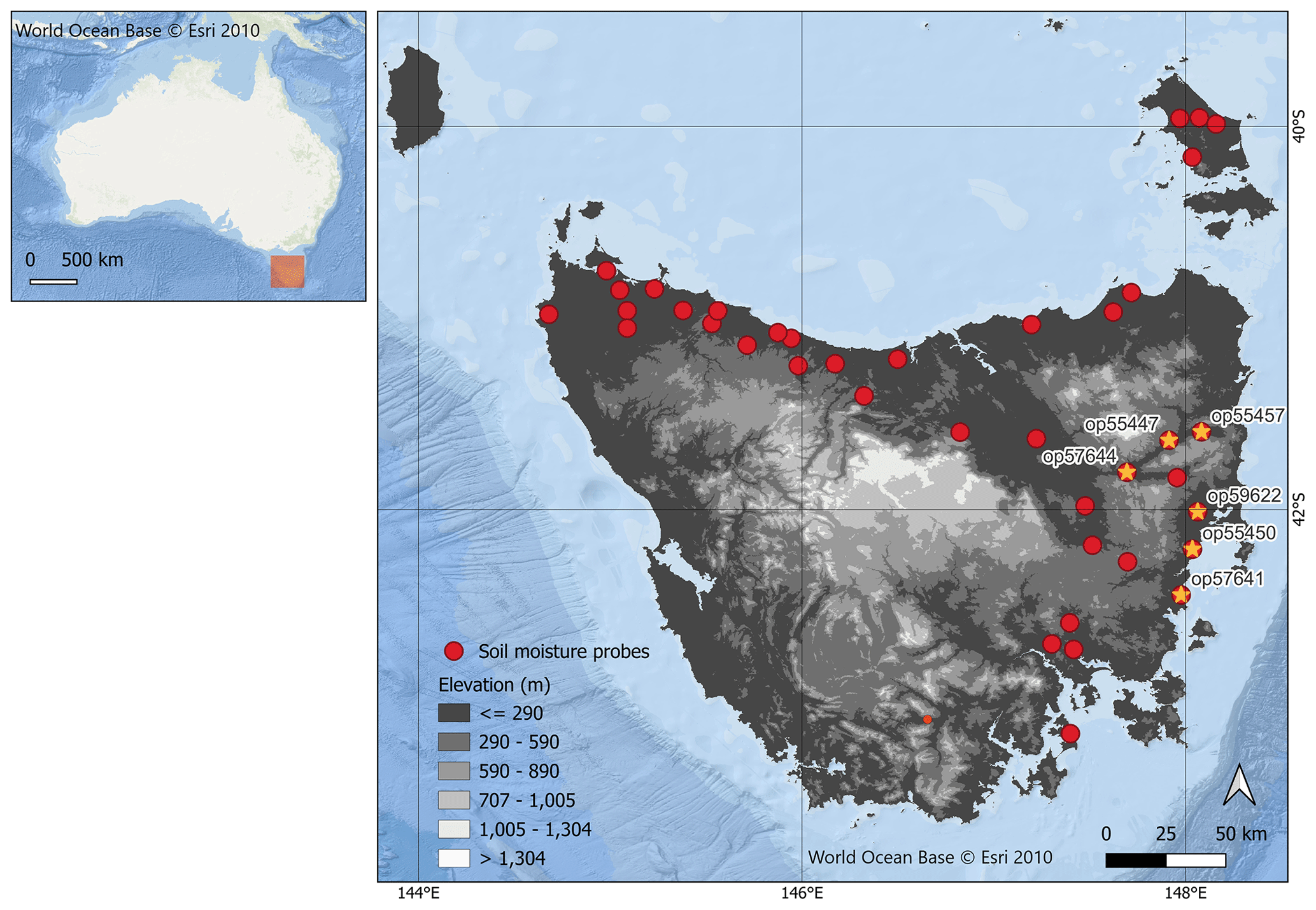
Figure 1 Elevation map of Tasmania. Red points represent soil moisture probes. The labeled points are stations that have recorded soil moisture data for more than 1 year.

2.2 Data sources

For the model development, we collected spatial data on parameters related to soil moisture from the Google Earth Engine database and Tasmanian geospatial layers. Soil moisture reference datasets were obtained from publicly available in situ and telemetered soil moisture measurements. We separated the Australia and Tasmania datasets. The detailed information on each dataset is summarized in Tables 1 and 2. Locations of the soil moisture stations are presented in Fig. 1 for Tasmania and in Fig. S1 in the Supplement for Australia. For Australia, data were collected from the OzFlux and OzNet databases. OzFlux provides SM data from the flux monitoring tower set up to understand the exchanges of carbon and water between terrestrial ecosystems and the atmosphere across Australia. OzFlux stations use a time domain reflectometry sensor to record moisture level at specific soil depths that vary among the stations (see the details at https://www.ozflux.org.au/, last access: 23 July 2023). Meanwhile, OzNet provides soil moisture records from several sites in the Murrumbidgee catchment, southern New South Wales, Australia. Each site measures soil moisture at 0–5 cm with a soil dielectric sensor (Stevens Hydraprobe^®) or 0–8, 0–30, 30–60, and 60–90 cm with water content reflectometers (Campbell Scientific) (Young et al., 2008).

For stations in Tasmania, soil moisture data were recorded using capacitance (EnviroPro) probes based on the frequency domain principle. Each device records a moisture value every 10 cm up to 80 cm soil depth with a frequency of 15 min.

Table 1 Sources of datasets as inputs for soil moisture modeling.

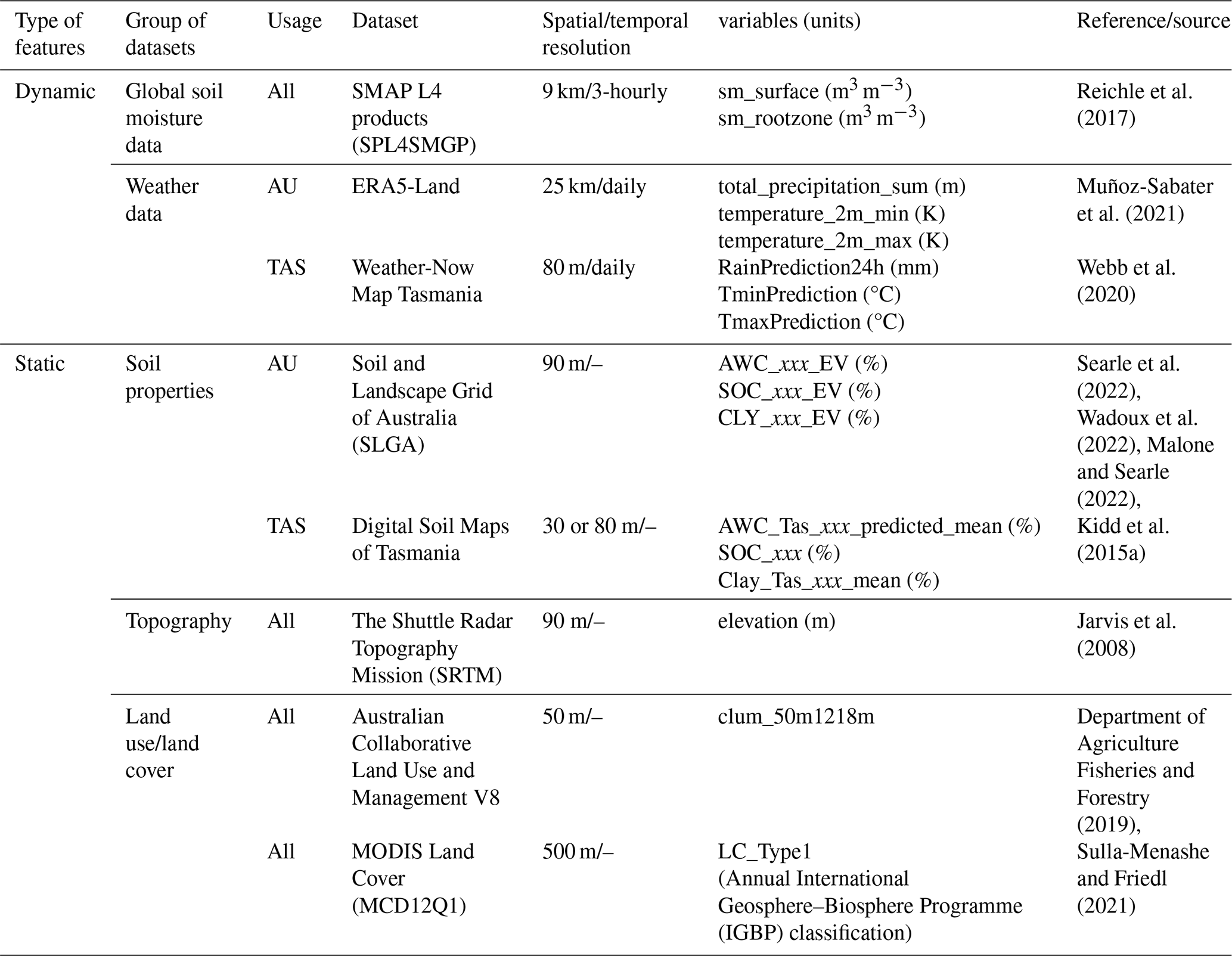
Note: xxx in soil datasets represents soil depth variation. Tmin=daily minimum air temperature, Tmax=daily maximum air temperature.

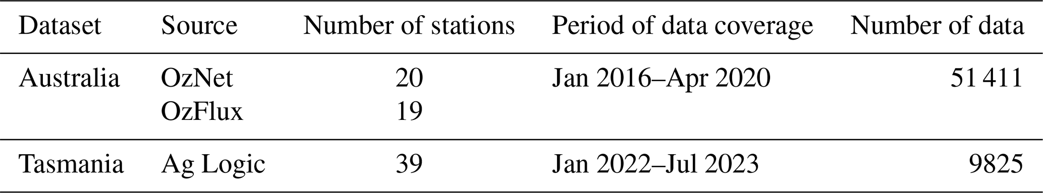
Table 2 Detailed information for the soil moisture data. The location of Australian stations used in this study can be found in the Supplement. “Number of data” refers to the dataset used for model training.

2.3 Deep learning approaches

In this work, we used three types of DL algorithms, which are multilayer perceptron, long-short term memory, and transfer learning, to develop soil moisture models. These algorithms were executed in Python using keras in the TensorFlow module (Abadi et al., 2015).

2.3.1 Multilayer perceptron

A multilayer perceptron (MLP) is a type of artificial neural network consisting of hidden layers between input and output layers (Park and Lek, 2016; Rumelhart et al., 1986). Each layer is connected by multiple perceptrons. A perceptron is a type of neuron with a logical threshold in producing an output value. In MLP, the weights attached to the input of perceptrons are combined into a weighted sum and become the base value against a threshold of whether the neuron will be activated. The threshold is set by an activation function.

Since the MLP algorithm contains more than one hidden layer, combinations of perceptrons between layers could resolve nonlinear relationships between input and output layers. The multilayer concept means that the perceptron's output values in one layer are propagated to the next layer as the input. At the end of the perceptron, the final output value is compared to the reference value and is evaluated using a cost function to quantify the difference between predicted and actual values. An optimization function is then used to minimize this difference metric. Additionally, this algorithm has a backpropagation scheme, which calculates the gradient error across all pairs of input and output into the first hidden layer and uses the gradient to update the weight values. All these processes are processed in an iteration or epoch. Detailed explanations of MLP as an advanced neural network can be found in Huang (2009).

2.3.2 Long short-term memory

Long short-term memory (LSTM) is a type of recurrent neural network (RNN) that overcomes the challenge of long-term dependency in regular RNN (Zhang et al., 2021). This approach is commonly applied to sequence datasets such as time series data (Lindemann et al., 2021). In one neuron of LSTM, there is a cell state representing the long-term memory responsible for filtering and controlling the information from input and other layers. This cell state decides which information will be stored and passed through as output and which information will be removed as it does not correlate with the function. There are two types of LSTM: unidirectional LSTM and bidirectional LSTM. The one-directional LSTM only stores information about the network that moves forward. Meanwhile, in bidirectional LSTM, the neural network can work in both forward and backward directions of the information flow. LSTM has been utilized for a wide range of problems, including soil moisture and soil temperature estimation (Li et al., 2023). The use of the LSTM approach in crop yield prediction research has been reviewed by Van Klompenburg et al. (2020) and Teixeira et al. (2023).

2.3.3 Transfer learning

Transfer learning (TL) is a technique in deep learning that transfers knowledge from a trained model to a new model that has a similar architecture (Lu et al., 2015). Theoretically, the new model does not need to be trained from scratch since the transferred knowledge has an overview pattern of the data. This can reduce training time or even increase the model's performance (Pan and Yang, 2010). A TL approach generally consists of three stages, which are (i) developing or selecting a pre-trained model, (ii) reusing the model, and (iii) fine tuning the model. A pre-trained model can be a globally accepted general model or a model developed based on a large dataset. Reusing the model means importing the weights of all or several layers from the pre-trained model to the new model. Fine tuning is the training process on the transferred new model using a new specific dataset. A clear illustration of how transfer learning works is presented in Padarian et al. (2019a).

2.4 Soil moisture modeling

2.4.1 Data preparation

Preparing datasets for model development included data cleaning of the reference soil moisture probes data, stacking images of covariates, and sampling the covariates based on probe locations. For the Tasmanian dataset, the recorded soil moisture data were in percentage values representing the proportion of water within the pore space in the soil. Since we need the proportion of water within the soil volume, we converted the measured data by multiplying them by total porosity calculated from bulk density (BD) values. The BD values were derived from the digital soil map of Tasmania extracted at each probe location. The Australian soil moisture dataset has been calibrated from each database source; thus, we use the values directly for analysis. We then calculated the measured moisture values at various depths into an aggregated mean value for the surface (0–30 cm) and subsurface (30–60 cm) soil layers. We applied the equal-area spline interpolation (Bishop et al., 1999) and calculated the average daily soil moisture from sub-hourly records. We also converted all soil moisture data in decimals of volumetric water content (m³ m⁻³).

Covariates were collected using the Google Earth Engine platform. We first stacked weather datasets, including daily accumulated rainfall and daily maximum and minimum temperature (Tmax and Tmin) as the reference date. Since rainfall has an extended effect on soil moisture levels, we included the current and the last 3 d of rainfall data in the covariate list. Thus, we had four layers of rainfall data for each day (RAIN_t, RAIN_t−1, RAIN_t−2, and RAIN_t−3).

Daily values of SMAP soil moisture were averaged, and we only selected the surface (surf_SMAP) and root zone bands (rootz_SMAP) representing 0–5 and 0–100 cm soil layers. Since SMAP-L4 products have a 3 d latency, we used backward 4–7 d windows to get the sequence of SMAP bands (SMAP_t, SMAP_t−1, …, SMAP_t−n with t as the day and n from 4 to 7 referring to the backward sequence). This series was then converted into a multiband image and stacked together with the weather data.

The multiband images of weather and SMAP data were then combined with land cover, elevation, and spatial soil property data. For the land cover, we used five categories, i.e., pasture, forest, rain-fed agricultural, savannah, and irrigation (PAST, FORE, AGRI, SAVA, and IRRI). FORE includes areas classified as native vegetation and native forest in CLUM or any type of forest defined in IGBP. Cropping and horticulture classes in CLUM are included in AGRI. The IRRI category covers area production from irrigated agriculture and plantations in the CLUM classification. SAVA includes areas defined as closed shrublands, woody savannahs, and savannahs in IGBP. The rest of the classes are categorized as PAST. We applied a one-hot-encoding method to convert land cover categories into a binary (zeros and ones) numerical format. Each class is represented as a separate column, where a value of 1 indicates the presence of that category, and 0 indicates its absence.

For soil properties, we selected three variables that affect the water storage of soils, including available water content (AWC), soil organic carbon (SOC), and clay content (CLY). Maps representing four layers of soil depth (0–5, 5–15, 15–30, and 30–60 cm) of each variable were incorporated as covariates. These were further named AWC_Lx, SOC_Lx, and CLY_Lx, with L being a layer and x an integer from 1 to 4.

Finally, the daily multiband image containing all covariates was generated based on the time frame of the Australian and Tasmanian datasets. Covariate values were then sampled at each location with measured soil moisture data, producing paired datasets of covariates and observed data for each date at every station. Any row that contained missing values in either covariates or observed data was excluded. This led to 51 411 observations covering the period of January 2016–April 2020 for the Australia dataset and 9825 observations for Tasmania from January 2022–July 2023.

2.4.2 Model setup

This study set the deep learning models to have two output values representing soil moisture for the surface and subsurface layers (0–30 and 30–60 cm, respectively). The structure of the MLP model consisted of four dense layers of 128, 64, 32, and 16 neurons as the hidden layer, existing in between the input and output layers. We used a Rectified Linear Unit (ReLU) and Adam optimizer as the activation and optimization functions, respectively. The learning rate, batch size, and number of epochs used in this algorithm were 0.0001, 128, and 150, respectively. To avoid overfitting in the training process, an early stopping was applied based on the validation loss, which halted the training if there was no improvement after five epochs.

For the LSTM algorithm, the time series dataset of SMAP was used as input in bidirectional LSTM. This part formed a 2×8 shape, which then passed through a dense layer of 100 neurons. Combined with the rest of the covariates, this became the input of four hidden layers with 128, 64, 32, and 16 neurons. To make a fair comparison, we set the activation and optimization functions, learning rate, batch size, and number of epochs in LSTM that are similar to the MLP.

During model training and validation, the value of 1−ρ_c (Lin's concordance correlation coefficient, Eq. 1) was used as a loss function. We aimed its minimum value for validation to get the best model performance. Lin's coefficient represents the distance of predicted data plotted against the observed data with the 45° line (Lin, 1989):

$$\begin{array}{}\text{(1)}& {\mathit{\rho }}_{\mathrm{c}}={\displaystyle \frac{\mathrm{2}{s}_{xy}}{s_x^{\mathrm{2}}+s_y^{\mathrm{2}}+(\stackrel{\mathrm{‾}}{x}-\stackrel{\mathrm{‾}}{y}{)}^{\mathrm{2}}}},\end{array}$$

where $s_x^{\mathrm{2}}$ and $s_y^{\mathrm{2}}$ are the variances, while $\stackrel{\mathrm{‾}}{x}$ and $\stackrel{\mathrm{‾}}{y}$ are the mean of the observed and the predicted soil moisture. s_xy is the covariance value calculated using Eq. (2):

$$\begin{array}{}\text{(2)}& s_{xy}={\displaystyle \frac{\mathrm{1}}{n}}\sum _{i=\mathrm{1}}^n(x_i-\stackrel{\mathrm{‾}}{x})(y_i-\stackrel{\mathrm{‾}}{y}),\end{array}$$

where n is the number of data, and i is the order of data being calculated. This function can represent how well the model captures temporal patterns of the observed data in a time series.

Figure 2 Soil moisture modeling scheme.

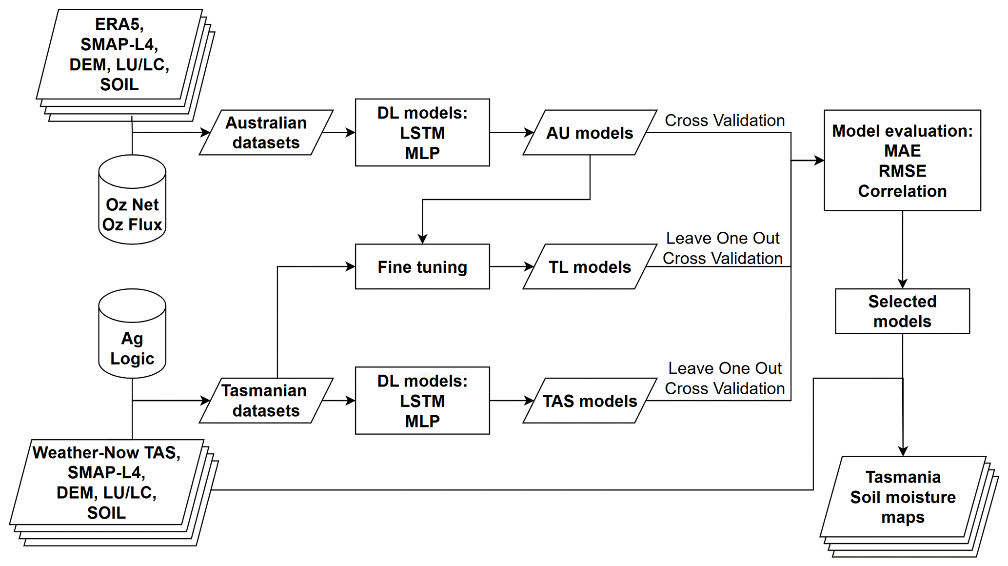
For analysis, we had three scenarios for feeding these two DL algorithms. Figure 2 shows the modeling scheme used in this study.

• a.

  The Australian (AU) model was trained on the Australian dataset. This was based on the model developed by Fuentes et al. (2022) with a modification of feature selection as model input: (1) used the most recent product of the SMAP dataset; (2) excluded variables having the least impact on DL predictions, which are the Sentinel-1 dataset, vegetation index, and land surface temperature; (3) added daily maximum and minimum air temperature. We derived only one AU model for each DL algorithm by splitting the dataset into 2016–2018 for training and 2019–2020 for validation.

• b.

  The Tasmanian (TAS) model was trained on the Tasmanian dataset. We derived multiple models for analysis using the leave-one-station-out cross-validation schema across 39 monitoring stations.

• c.

  The transfer learning (TL) model was also used. Here, we used the trained AU model and fine-tuned the model using the Tasmanian dataset. For MLP, we transferred the weights of the first three hidden layers of the AU model and kept them unchanged during the fine-tuning process. Meanwhile, for LSTM, we kept the first three hidden layers after LSTM output (128, 64, and 32 neuron layers) unchanged. The rest of the neurons, including the weights on LSTM architecture, were retrained.

2.4.3 Model evaluation

An evaluation was first conducted on AU models. We applied AU models to predict soil moisture in Tasmania and quantified the goodness of fit between predicted and measured values. Subsequently, the TAS and TL models were evaluated using the leave-one-station-out cross-validation (CV) testing scheme. This scheme comprised randomly selecting one station as a testing set, another station as a validation set, and the rest of the stations as the training set. The scheme was applied to all probes, thus resulting in 39 models for each of the TAS and TL models.

The goodness of fit between the prediction and observations was quantified based on mean absolute error (MAE), root mean square error (RMSE), and Pearson's linear correlation coefficient (Eqs. 3–5).

$$\begin{array}{}\text{(3)}& {\displaystyle }& {\displaystyle }\text{MAE}={\displaystyle \frac{{\sum }_{i=\mathrm{1}}^n|y_i-x_i|}{n}}\text{(4)}& {\displaystyle }& {\displaystyle }\text{RMSE}=\sqrt{\sum _{i=\mathrm{1}}^n{\displaystyle \frac{(y_i-x_i{)}^{\mathrm{2}}}{n}}}\text{(5)}& {\displaystyle }& {\displaystyle }r={\displaystyle \frac{{\sum }_{i=\mathrm{1}}^n(x_i-\stackrel{\mathrm{‾}}{x})(y_i-\stackrel{\mathrm{‾}}{y})}{\sqrt{{\sum }_{i=\mathrm{1}}^n(x_i-\stackrel{\mathrm{‾}}{x}{)}^{\mathrm{2}}}\sqrt{{\sum }_{i=\mathrm{1}}^n(y_i-\stackrel{\mathrm{‾}}{y}{)}^{\mathrm{2}}}}}\end{array}$$

Here, y_i is moisture prediction, x_i is an observation, and n is the amount of data. The final Tasmanian soil moisture maps were calculated from the average of 39 maps derived from the leave-one-station-out CV schema using the LSTM-TL algorithm. We also calculated the standard deviation from this model output to show the model's uncertainty.

2.4.4 Model interpretation

To explain the contribution of each input variable in soil moisture prediction, we calculated the Shapley value (Aas et al., 2021). The Shapley value is the marginal contribution of each predictor after considering all possible combinations. The SHAP value is derived from game theory and optimal Shapley values and has been widely used to interpret feature contribution in deep learning models (Padarian et al., 2020; Odebiri et al., 2022; Mohammadifar et al., 2022). In this study, SHAP calculation was based on the transferred LSTM model with a random split of 0.9:0.1 for training and testing. SHAP values resulting from the testing dataset were summed across different times or covariates for analysis. The calculation was done using the Shapley Additive exPlanations (SHAP) library in Python language (Lundberg and Lee, 2017).

3 Results

3.1 Distribution of moisture data

We first compared the soil moisture (SM) data from the Australian and Tasmanian datasets that were used for building the DL models. Figure 3 shows the distribution of SM data over the analysis period based on density probability and histogram plots. The Tasmanian data generally had a similar pattern to that of the Australian data. Both types of data were left-skewed for the surface layer and had a peak concentration of around 0.2 m³ m⁻³. Nevertheless, the Tasmanian data were slightly shifted to the right with a mean value of 0.26 m³ m⁻³ higher than the Australian one ($\text{mean}=\mathrm{0.17}{\mathrm{m}}^{\mathrm{3}}{\mathrm{m}}^{-\mathrm{3}}$). The Tasmanian data ranged from 0.07 to 0.54 m³ m⁻³, while the Australian data ranged 0.02–0.50 m³ m⁻³. The Tasmanian data showed a lower density value for soil moisture below 0.2 m³ m⁻³ compared to the Australian data but exhibited higher concentrations above 0.25 m³ m⁻³.

Figure 3 Distribution plot of the Australian (AU) and Tasmanian (TAS) soil moisture data.

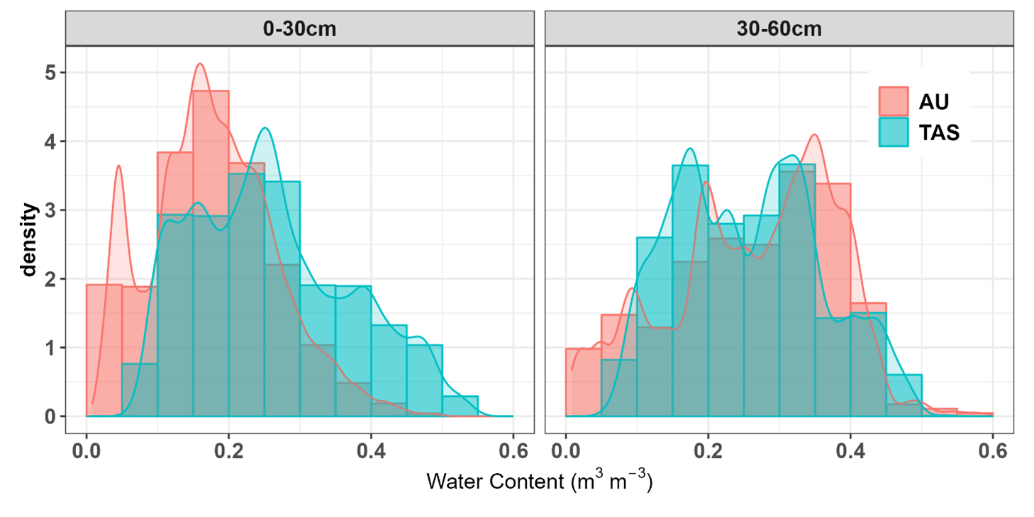
Meanwhile, for subsurface soil moisture data, both regions showed two peaks of data concentration (about 0.20 and 0.35 m³ m⁻³) yet different types of distribution. The Australian data were relatively skewed to the right (skewness −0.32), while the Tasmanian data were skewed to the left (skewness 0.23). The Australian data for this layer had a wider range (0.01–0.60 m³ m⁻³) compared to the Tasmanian data (0.06–0.54 m³ m⁻³). The Tasmanian data had more concentrations around 0.10–0.35 m³ m⁻³, while the Australian data had a fair distribution of moisture levels below 0.30 m³ m⁻³. Despite these differences, both types of subsurface data had a similar mean value of about 0.26 m³ m⁻³.

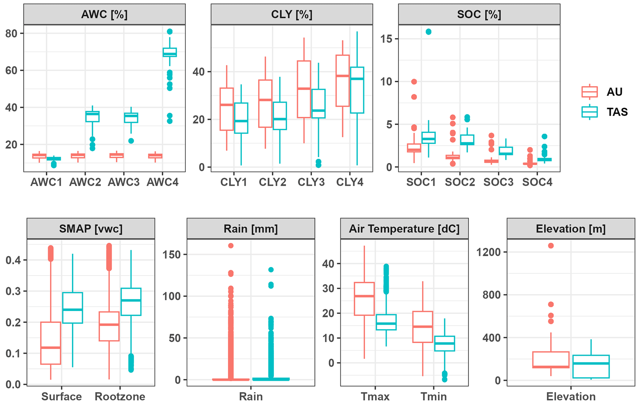
Figure 4 Comparison of the box plot from the Australian (AU) and Tasmanian (TAS) covariates used in this study, including available water content (AWC), clay content (CLY), soil organic carbon (SOC), soil moisture (in volumetric water content, m³ m⁻³) from SMAP, rainfall, air temperature, and elevation. The number next to soil properties refers to the soil layer of 0–5, 5–15, 15–30, and 30–60 cm depths.

We also plotted the distribution of data of each covariate for Australia and Tasmania (Fig. 4). The Australian soil data generally had lower values of available water and carbon content than the Tasmanian data. Soil moisture values extracted from the global SMAP dataset for Australia had lower mean values for both the surface and subsurface soil layers, yet they had a wider range of moisture levels. For the rest of the covariates (weather data and elevation), the Australian data covered a larger range of values than in Tasmania. The maximum rainfall data in Australia reached 160 mm d⁻¹, while in Tasmania it was up to 131 mm d⁻¹. The distribution of air temperature data also followed the same trend, with Tasmania having lower mean values for both the daily maximum and minimum.

3.2 SMAP prediction of soil moisture in Tasmania

Soil moisture content from the SMAP dataset was used as the primary covariate in our models. We first investigated the relationship between SMAP and field-observed soil moisture in Tasmania. Surface soil moisture of SMAP (0–5 cm) was directly compared to the first level of measurement (10 cm depth), while the SMAP root zone (0–100 cm) was against the average moisture values of all level measurements (10–80 cm depths). The overall correlation coefficient between SMAP and measured data was 0.37 for the surface and 0.49 for the root zone layer. SMAP SM data had a moderately high correlation coefficient with the measured data across different stations in Tasmania, with median values of 0.77 and 0.76 for the surface and root zone layer, respectively. The difference between SMAP and ground measurements for the root zone ($\text{MAE}=\mathrm{0.08}{\mathrm{m}}^{\mathrm{3}}{\mathrm{m}}^{-\mathrm{3}}$ and $\text{RMSE}=\mathrm{0.10}{\mathrm{m}}^{\mathrm{3}}{\mathrm{m}}^{-\mathrm{3}}$) was slightly lower than for the surface ($\text{MAE}=\mathrm{0.09}{\mathrm{m}}^{\mathrm{3}}{\mathrm{m}}^{-\mathrm{3}}$ and $\text{RMSE}=\mathrm{0.11}{\mathrm{m}}^{\mathrm{3}}{\mathrm{m}}^{-\mathrm{3}}$). According to the distribution of errors and correlation coefficients across the measuring stations, SMAP of the root zone layer had a wider range of errors and correlation coefficients compared to the surface layer (Fig. 5). In addition, there were more stations with negative correlation values for the root zone SMAP.

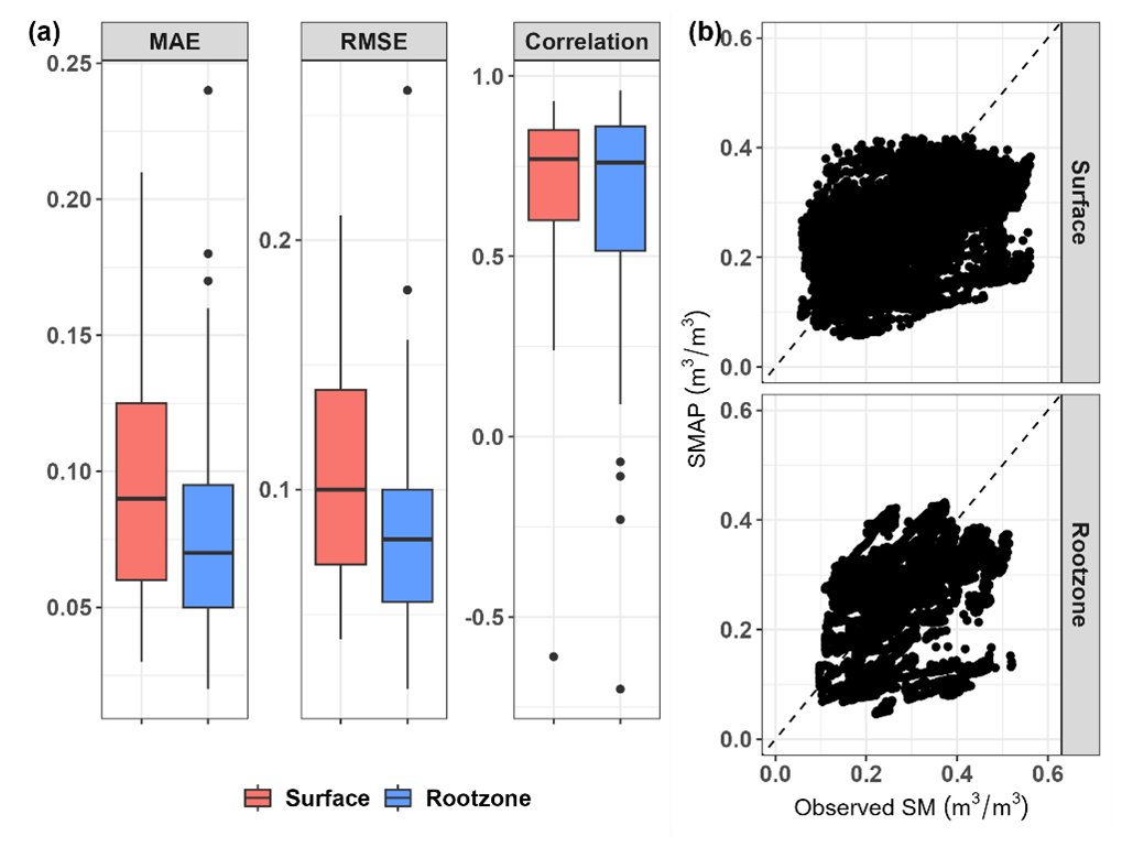
Figure 5 Performance of soil moisture derived from the SMAP dataset compared to measured data in Tasmania during the period of January 2022–April 2023: (a) the distribution of mean absolute error (MAE), root mean square error (RMSE), and correlation value at each probe location. (b) Overall performance on the scatter plot between predicted and measured soil moisture data compared to the 1:1 line (dashed line).

3.3 Model selection and performances

We evaluated the performance of deep learning models, calibrated with Australian data (referred to as Australian models), in predicting soil moisture levels in Tasmania. The models' predictions were compared to measurements of each station. In general, models with the MLP approach performed better than LSTM for both the surface and subsurface layers, with the MLP having an average MAE of 0.1m³ m⁻³, RMSE of 0.12 m³ m⁻³, and correlation of 0.49 compared to LSTM with an average MAE of 0.12 m³ m⁻³, RMSE of 0.15 m³ m⁻³, and correlation of 0.48 (Fig. 6). The MLP model resulted in predictions that were closer to the 45° line with the observed data. Furthermore, according to the distribution of performance across Tasmanian stations, the MLP model predictions had lower errors and less variation, as shown by the box plot. The LSTM model had good correlation coefficients (>0.6) in most stations. However, despite the promising performance of the MLP algorithm, the models did not demonstrate any improvement in prediction accuracy over using just the SMAP dataset alone (Fig. 5).

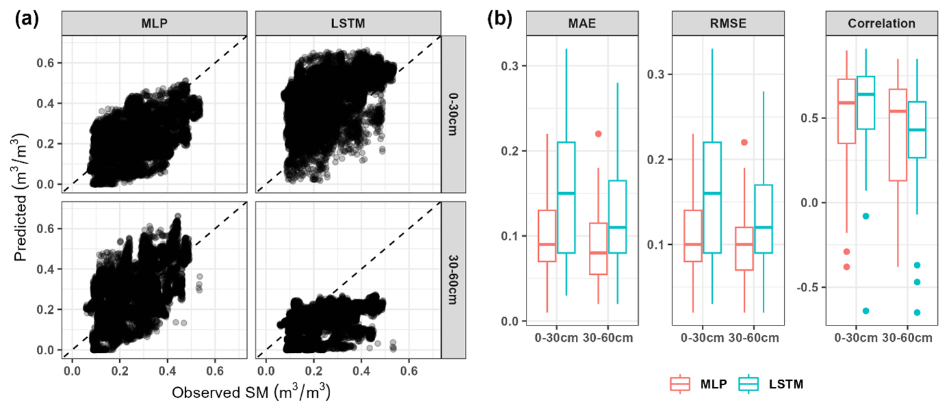
Figure 6 Performance of Australian models for soil moisture prediction in Tasmania based on multilayer perceptron (MLP) and long-short term memory (LSTM) approaches: (a) overall comparison between predicted and observed soil moisture data and the (b) distribution of mean absolute error (MAE), root mean square error (RMSE), and correlation value across 39 stations in Tasmania.

Thus, the second set of models was trained on Tasmanian data using the leave-one-station-out cross-validation scheme. The results show that the predicted soil moisture varied from 0 to 0.8 m³ m⁻³, giving a larger range than the observed data (Fig. 7). The scatter plots of predictions and observations show a large dispersion, with some zero-value predictions regardless of the variation of the observed data. Both DL approaches had similar results in performance valuation. The MLP models were slightly better than LSTM, with average MAE of 0.12 m³ m⁻³, RMSE of 0.15 m³ m⁻³, and correlation of 0.43, while the LSTM models had MAE of 0.13 m³ m⁻³, RMSE of 0.17 m³ m⁻³, and correlation of 0.26. Model evaluation for each station showed that the error values and correlation of both DL models for subsurface soil moisture prediction (0.01–0.48 m³ m⁻³ for MAE and RMSE; −0.63 to 0.96 for correlation) were more varied compared to surface moisture predictions (0.02–0.35 m³ m⁻³ for MAE and RMSE; −0.07 to 0.94 for correlation).

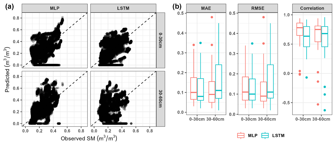
Figure 7 Performance of Tasmanian models for soil moisture prediction in Tasmania based on multilayer perceptron (MLP) and long-short term memory (LSTM) approaches: (a) overall comparison between predicted and observed soil moisture data and the (b) distribution of mean absolute error (MAE), root mean square error (RMSE), and correlation value across 39 stations in Tasmania based on a leave-one-out cross-validation scheme.

Finally, the transfer learning approach was deployed by transferring knowledge from the trained Australian models to Tasmania. Visually, data points resulting from TL models against the observed data were closer to the 45° line for both MLP and LSTM (Fig. 8). The predicted data for MLP were in the range of 0 up to 0.7 m³ m⁻³, which is larger than that of LSTM (0.03–0.63 m³ m⁻³). The overall performance of LSTM models showed MAE of 0.07 m³ m⁻³, RMSE of 0.08 m³ m⁻³, and correlation of 0.73. This was slightly better than the performance of the MLP models, with average MAE, RMSE, and correlation of 0.08 m³ m⁻³, 0.09 m³ m⁻³, and 0.62. The distribution of model performance for both DL algorithms on predicting soil moisture across all stations in Tasmania was quite similar. However, the LSTM model with transfer learning had a more consistent performance for the surface and subsurface layer, as shown by the upper quartile of the box plot for errors. The results indicate that most stations had error values less than 0.08 m³ m⁻³ for surface and subsurface predictions.

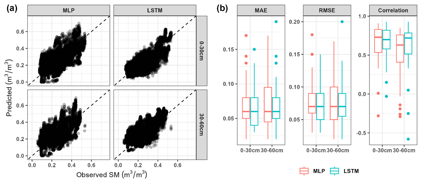
Figure 8 Performance of transfer learning models for soil moisture prediction in Tasmania based on multilayer perceptron (MLP) and long-short term memory (LSTM) approaches: (a) overall comparison between predicted and observed soil moisture data and the (b) distribution of mean absolute error (MAE), root mean square error (RMSE), and correlation value across 39 stations in Tasmania based on a leave-one-out cross-validation scheme.

Comparing the performance of the six models for predicting SM in Tasmania, it becomes evident that the LSTM with the transfer learning approach (LSTM-TL) was optimal. We further analyzed its performance according to station locations, time series, land cover types, and seasonal time.

The spatial distribution of the performance of the LSTM-TL model using different stations is shown in Fig. 9. Stations with high correlation values (>0.74) mostly corresponded to lower error, with RMSE lower than 0.087 m³ m⁻³. Meanwhile, stations with large errors ($\text{RMSE}>\mathrm{0.106}{\mathrm{m}}^{\mathrm{3}}{\mathrm{m}}^{-\mathrm{3}}$) had moderate to high correlation coefficients (>0.55). In addition, the stations with the lowest correlations had RMSE ranging from 0.068 to 0.106 m³ m⁻³.

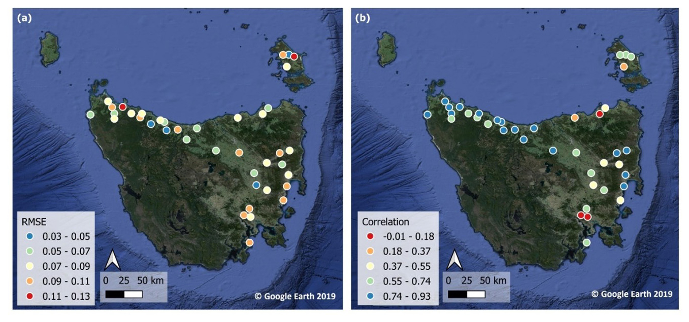
Figure 9 Spatial distribution of the performance of the long short-term memory (LSTM) model with transfer learning for predicting soil moisture at each station in Tasmania. The evaluations are an average of (a) root mean square error (RMSE) and (b) Pearson's correlation coefficient across the surface (0–30 cm) and subsurface (30–60 cm) soil layers.

Time series predictions for six typical stations compared to SMAP and observed data are plotted in Fig. 10. These cases show that our model predictions follow the dynamics of the observed data, with correlation coefficients varying from 0.43–0.84 for the surface layer and 0.35–0.85 for the subsurface layer. Our moisture predictions were relatively lower than the value from SMAP, yet the predictions better matched the observed data.

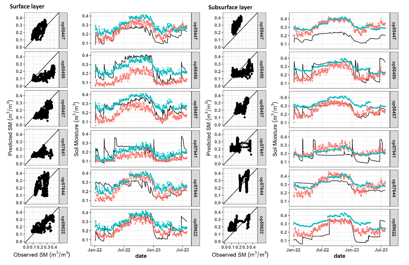
Figure 10 Performance of model results from the leave-one-station-out validation scheme for six stations with the longest observation periods: op55447, op55450, op55457, op57641, op57644, and op59622. The right panel shows the prediction of the entire series (red dots) compared to SMAP predictions (blue dots) and the observed data (black line). Note that SMAP predictions in the surface panel represent 0–5 cm, while the subsurface panel refers to 0–100 cm.

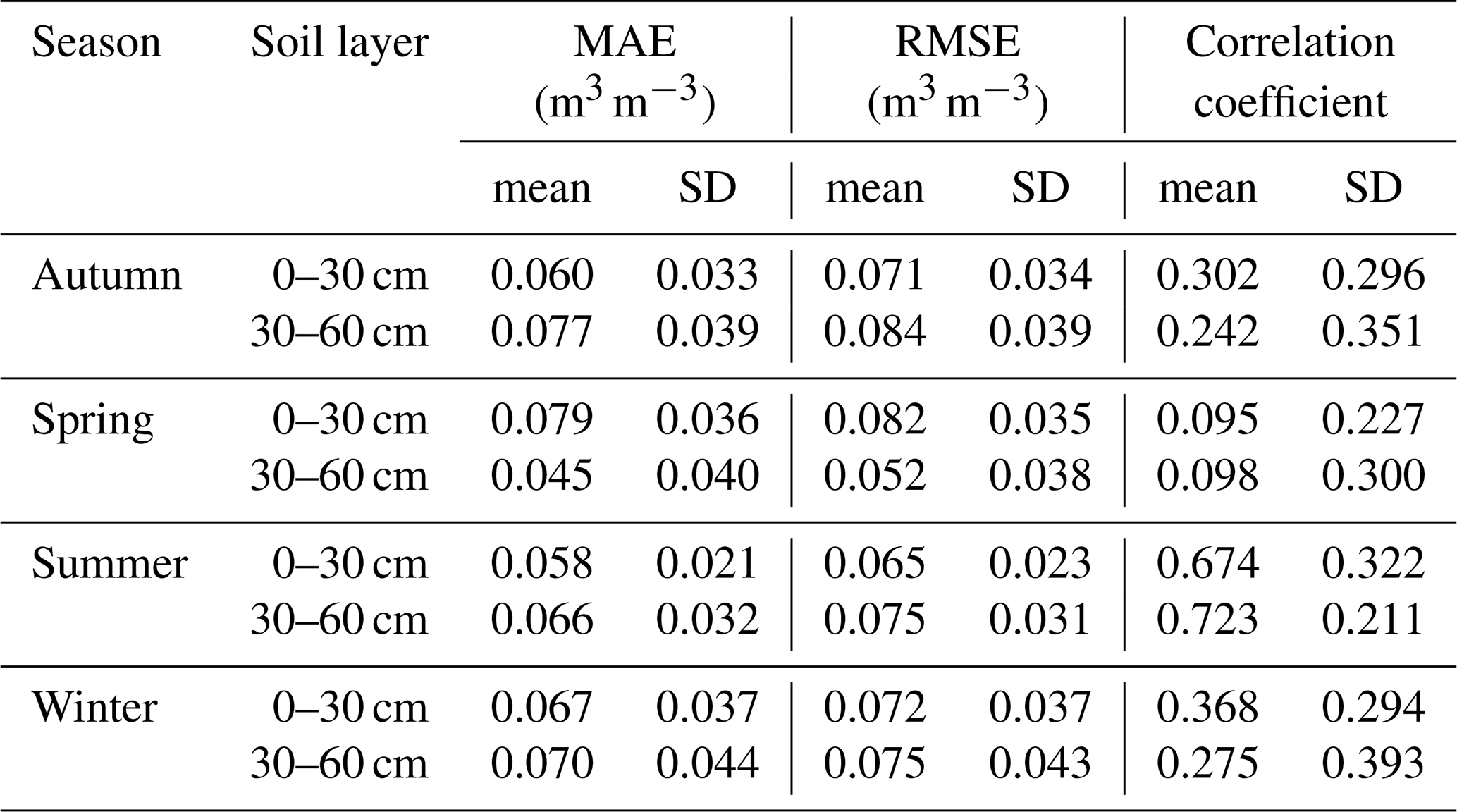
Table 3 highlights our model performance based on seasonal variations. The most accurate performance was achieved during summer, with an average correlation coefficient up to 0.72 and RMSE values around 0.06 m³ m⁻³. In other seasons, our model performed at MAE values ranging from 0.045 to 0.079 m³ m⁻³, with RMSE at 0.052 to 0.082 m³ m⁻³. Spring was identified as having a low correlation in both soil layers.

Table 3 Model performance during four seasons in Tasmania. The values were aggregated from all stations. MAE: mean absolute error, RMSE: root mean square error.

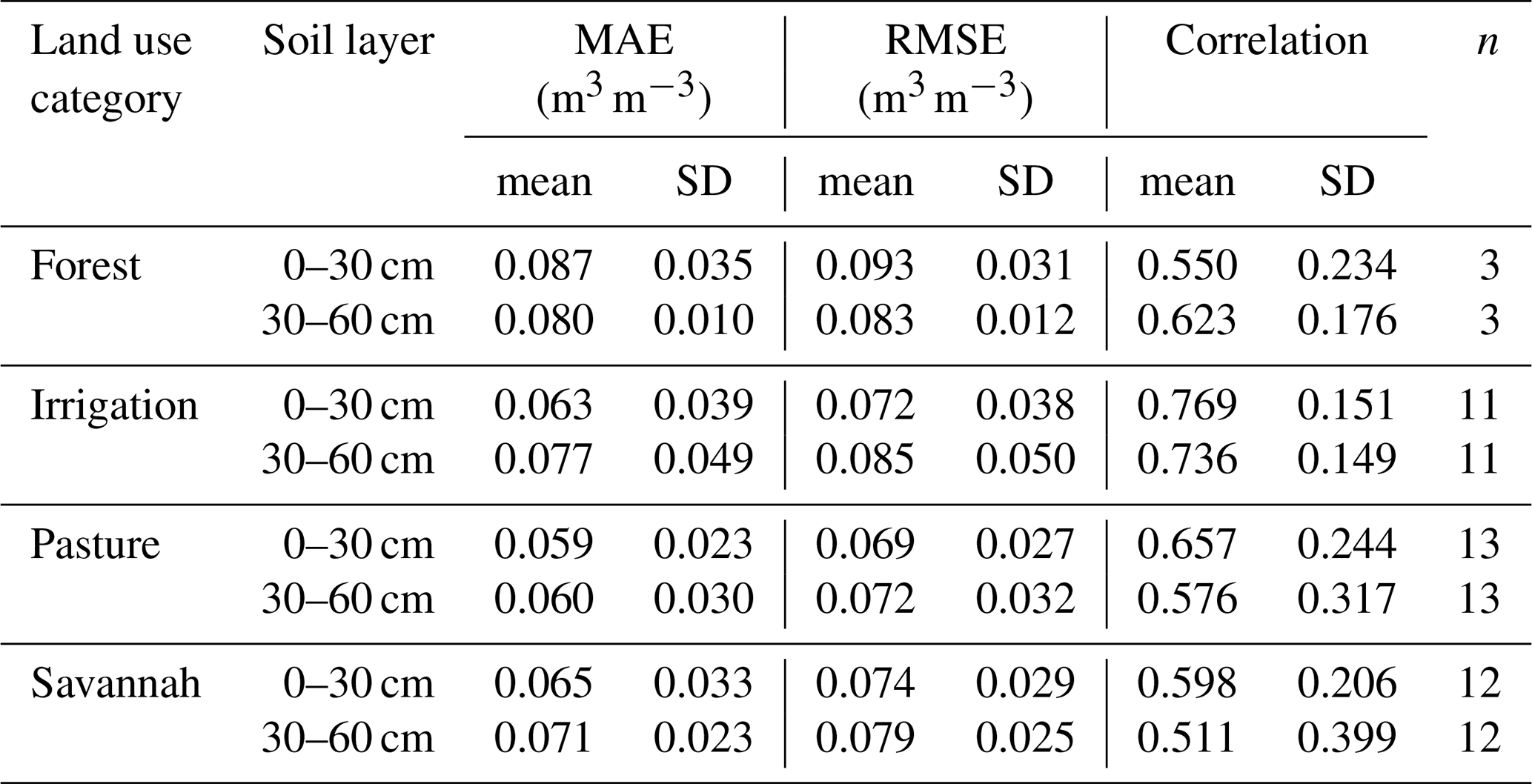
We also checked how our selected model performs in different land use categories (Table 4). Overall, the prediction consistently resulted in error values of 0.06 up to 0.09 m³ m⁻³ and correlation coefficients between 0.51 and 0.76 for both soil layers. Soil moisture prediction on the pasture area performed best, with the lowest error values ($\text{RMSE}=\mathrm{0.07}{\mathrm{m}}^{\mathrm{3}}{\mathrm{m}}^{-\mathrm{3}}$) and a high correlation coefficient (0.62). Forested area (with fewer stations) had the lowest correlation (0.550 and 0.623 for the surface and subsurface), followed by savannah (0.598 and 0.511 for the surface and subsurface).

Table 4 Performance of the selected model for predicting soil moisture in both soil layers aggregated by land use and land cover class (mean and standard deviation). MAE: mean absolute error, RMSE: root mean square error, n: number of stations.

3.4 Spatial pattern of predicted soil moisture

We then applied our calibrated models to predict soil moisture for the whole area of Tasmania at a daily time step and aggregated the values for each season (Fig. 11). High soil moisture occurred in the western part of Tasmania and small forested areas in the northeast. However, the western part was predicted as the driest area at the subsurface layer in all seasons. Our models estimated subsurface soil moisture at 0.01 to 0.55 m³ m⁻³ during the summer–autumn and up to 0.62 m³ m⁻³during the winter–spring. The average on the standard deviation maps varied up to 0.08 m³ m⁻³ for both soil layer predictions. In most of the high-moisture-level areas (near 1 m³ m⁻³), the deviation maps show the lowest value for surface moisture prediction. Higher deviation was identified in the central highland areas and hilly regions in the east and northeast. Meanwhile, the deviation map for subsurface soil moisture prediction depicts a higher uncertainty model over the western part of the state.

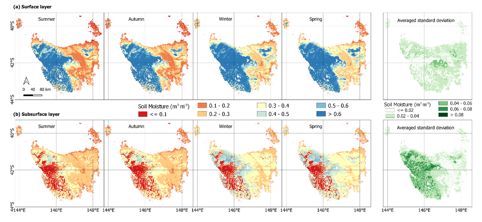
Figure 11 Spatial pattern of seasonal average predicted soil moisture along with its averaged standard deviation in Tasmania for (a) surface (0–30 cm) and (b) subsurface (30–60 cm) layers using LSTM models with the transfer learning approach. Soil moisture values are in m³ m⁻³.

An example of the 80 m resolution soil moisture maps for each soil layer and their uncertainty values over an area in the eastern part of Tasmania is given in Fig. 12. The Fingal Valley region encompasses agricultural lands with irrigation systems, including identifiable center pivot systems, distributed along the river between mountainous areas. The surface soil moisture map effectively captured topographical variations, as indicated by distinct color differences between the mountainous areas and their surroundings. Agricultural areas had lower moisture values (orange color), whereas higher values were predicted in mountainous areas. The uncertainty values were mostly less than 0.025 m³ m⁻³, except for the high-elevation area. Similarly, subsurface predictions can represent the spatial variation of the area of interest, particularly in irrigation areas and rivers. The uncertainty was more varied than the surface prediction, with no clear spatial pattern.

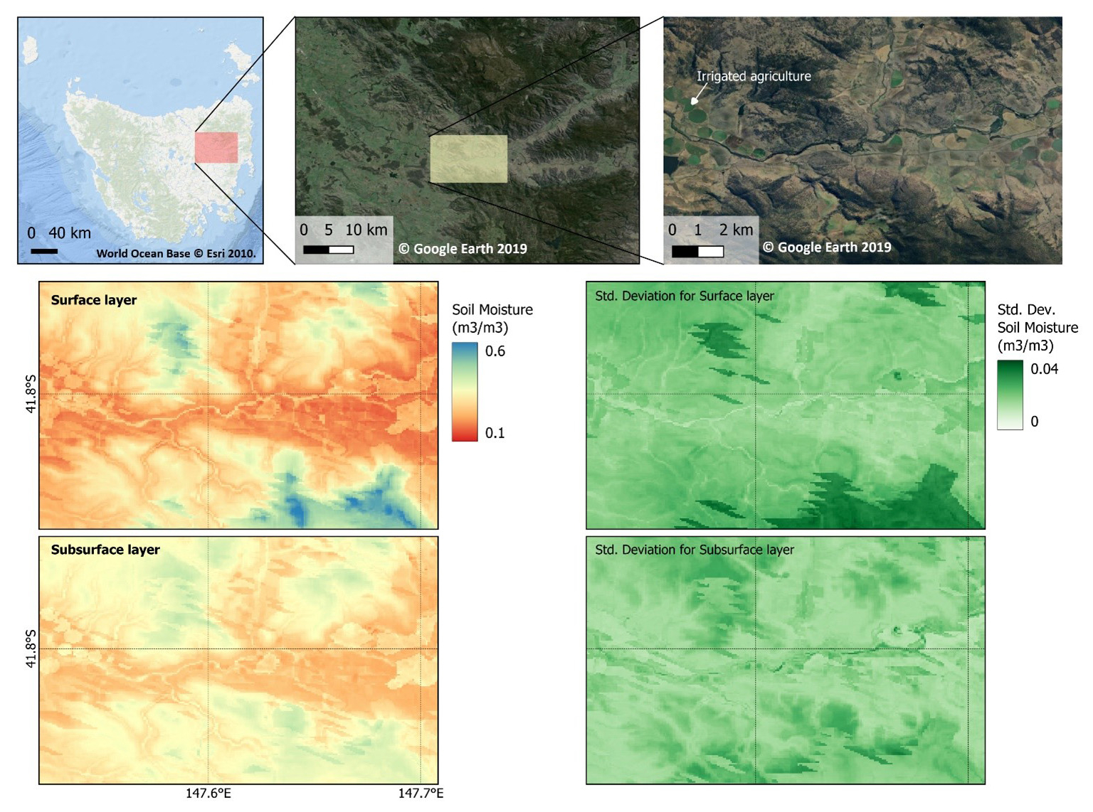
Figure 12 Soil moisture predictions and its standard deviation for surface and subsurface layers on 10 September 2023 as an example of an 80 m resolution map. The zoomed panel represents an area of the Fingal Valley.

3.5 Feature contribution

The importance of each input variable for the LSTM transfer learning model outputs was analyzed using the SHAP value. The violin plot (Fig. 13) summarizes three pieces of information: (1) overall comparisons in feature importance, (2) the distribution and variability of the SHAP value of each feature, and (3) the value of the feature shown by color scaling from low to high. Based on the testing dataset (n=884), it indicates that the SMAP dataset was the most important feature in predicting both surface and subsurface soil moisture. These were followed by LU/LC (land use and land cover) and soil properties (SOC and clay content). Elevation and weather data, including temperature and rainfall, were the least important covariates in our models. The SMAP surface had the widest range of SHAP values varying from −0.25 to 0.35. A high density of SMAP SM surface occurred in negative SHAP values, implying a reduction of the model output. High soil moisture in the SMAP surface gave additional value to the output prediction. However, the SMAP root zone had a reverse pattern, with a fair distribution of SHAP values ranging from −0.2 to 0.2; high soil moisture in the SMAP root zone negatively impacted the model output, and vice versa. Other covariates had less impact on the model output with SHAP values within −0.1 to 0.1. Land use and daily minimum air temperature predominantly gave a positive impact on the output.

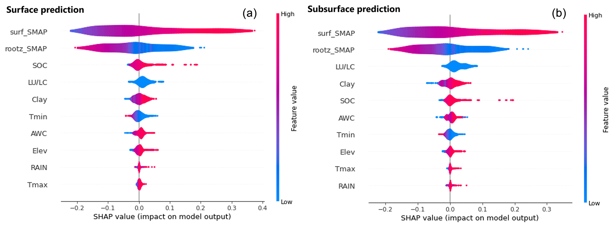
Figure 13 Aggregated SHAP value for each input dataset representing its impact on surface (left) and subsurface (right) soil moisture prediction based on the LSTM with the transfer learning model.

4 Discussion

4.1 MLP and LSTM approaches

We compared the MLP and LSTM as modeling algorithms to predict surface and subsurface soil moisture simultaneously. Our results revealed that MLP outperformed LSTM when directly applied to the Australian models to predict Tasmania soil moisture, yet contradictory results were found when using TL models. Nevertheless, both algorithms with the TL approach were equally good in predicting SM (Fig. 8). In the case of Australian models, the LSTM only records the “memory” of how the previous moisture and rainfall change daily soil moisture in Australia. When the LSTM is directly used to process SMAP in Tasmania, the memory of the Australian data might not apply in Tasmania, causing a larger error. In transfer learning, we let the weight of each cell in LSTM change during a fine-tuning process. This means that the model can update its memory of daily SMAP according to the Tasmanian dataset.

We chose the LSTM approach as our final model as it provides consistent results in predicting surface and subsurface soil moisture. Fuentes et al. (2022) compared the performance of LSTM and MLP in Australia. Their MLP models resulted in a slightly lower error compared to the LSTM, yet they chose the concatenated LSTM over stand-alone MLP as the recurrent neural networks could capture the delayed effect of soil moisture change occurring between soil layers. Another research study comparing LSTM and MLP to forecast soil moisture up to 6 d ahead in multilayers of soil showed that the LSTM model consistently resulted in a lower RMSE value (less than 0.09) (Han et al., 2021). However, we noted that their study used one output value for each soil layer, not implementing simultaneous predictions. Additionally, the LSTM approach has been widely investigated to model soil moisture with reliable performances in terms of spatial, time series, and forecast analysis (Li et al., 2022a; Park et al., 2023; Fang and Shen, 2020; Datta and Faroughi, 2023).

4.2 Comparing Australia, Tasmania, and transfer learning models

Based on our three scenarios, Australian models (AU) performed the worst regardless of the type of deep learning approach. High error in AU predictions was likely due to the differing value distributions between the Australian and Tasmanian datasets. These results further indicate that the direct application of deep learning models to other local areas necessitates careful consideration of data similarity. Comparing the performance of the Tasmanian (TAS) and the transfer learning (TL) models, TL models resolved the drawback of the TAS model, which could not fully capture the variations across Tasmania. As illustrated in Fig. 7, the TAS models exhibited shortcomings in predicting soil moisture, notably yielding zero values in some conditions. This outcome suggests that based on data from 39 stations, the model's training was inadequate in encompassing the full range of variability within the testing dataset. Consequently, this limitation hindered the TAS model's capacity to estimate soil moisture values when confronted with input values that extend beyond the scope of the training dataset. The small sample size in the training dataset may have limited the model's ability to generalize over Tasmania's major landscapes, topographical features, and soil properties.

To address this issue, the TL models effectively assimilated knowledge from the more extensive Australian dataset, resulting in a substantial enhancement in the performance of the TAS model. This approach significantly enhanced the training of the TL model, as it only required adjustments to the previously learned weight values to align them with the characteristics of the Tasmanian dataset. In contrast, the TAS model required a complete training process from scratch, with random values assigned to the weights of the DL layers as the initial conditions.

Adopting a transfer learning approach has shown significant potential for enhancing both training effectiveness and model performance. Our TL models, in particular, exhibited remarkable performance improvements, surpassing the TAS models by a factor of 2. This translated to error reductions of up to 45 % and a 50 % increase in correlation coefficients. Furthermore, these enhancements were consistently reflected in the accurate prediction of both surface and subsurface soil moisture levels.

The efficacy of transfer learning has been explored for several applications; for example, Li et al. (2021) demonstrate that employing transferred DL models based on ERA5-land data led to a substantial increase in the explained variation of observed data, exceeding 20 % in some areas of China. Padarian et al. (2019a) also reported that the transferred local model, designed for predicting soil properties from infrared spectra, outperformed both individually trained global and local models.

4.3 Spatiotemporal variation of predicted soil moisture

Soil moisture maps for Tasmania were generated using the LSTM with transfer learning models (Fig. 12). At an 80 m resolution, the model's performance is on par with the original models designed for 90 m soil moisture predictions in Australia (Fuentes et al., 2022). Nevertheless, there were still some limitations of the spatiotemporal coverage. Some stations with less than 1 year of observational data could give strange results when evaluating models' performance. This is shown by some stations, mainly with observational data for less than 3 months, that also have high correlation yet high error (Fig. 9).

While the map effectively captured the SM variation of the eastern part of Tasmania, our predictions struggled to capture the variability of SM in the rocky, mountainous areas in the western part of Tasmania (Fig. 1). This limitation is due to the absence of observational data in these remote regions, meaning that our model lacked the necessary information to learn and make accurate predictions. The western part of Tasmania has soil organic carbon (SOC) content exceeding 20 % (Kidd et al., 2015a). These peatlands with high SOC levels surpassed the maximum value of SOC present in our training dataset, which had a maximum of 15 %. As a consequence, our models produced very high moisture values (near 1) for surface predictions and small values (near 0) for subsurface predictions. The SHAP value indicated that SOC contributed significantly to the soil moisture prediction in this area, overshadowing the contribution of the SMAP dataset (refer to Fig. 14). Those results align with the low predicted soil thickness (<50 cm) across western Tasmania (Kidd et al., 2015a), which certainly contributed to the low moisture level in the subsurface layer.

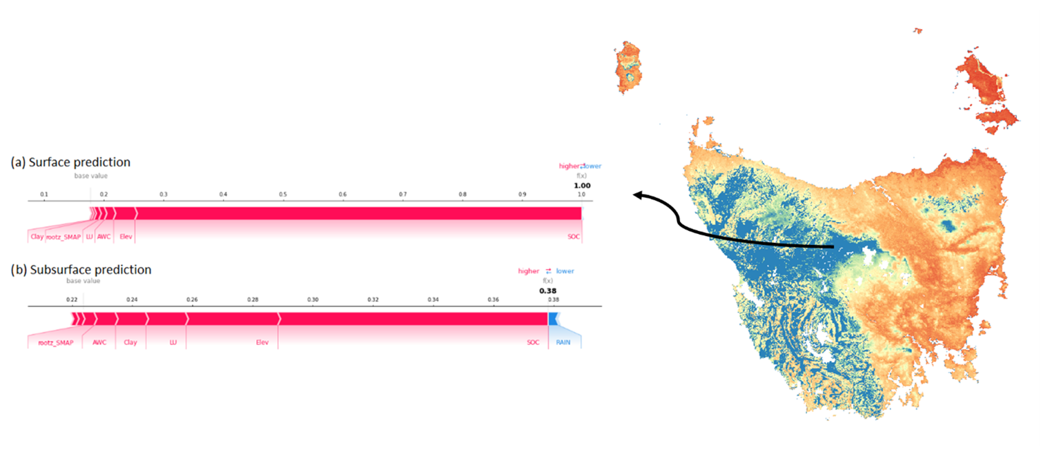
Figure 14 An illustration of feature contributions in generating soil moisture prediction in remote areas. The base value represents the average of model output over the training set specifically for SHAP analysis, while f(x) is the final prediction of the soil moisture value.

4.4 Assumptions and limitations

While we demonstrated the ability of the transfer learning model to accurately predict soil moisture using a leave-one-station-out testing protocol, we recognize some assumptions and limitations of the study. We assumed that our reference data represent actual moisture level values in each soil layer, but there are possible biases from the interpolation and calibration procedure on recorded data from the probes. Moreover, the limited number of stations (6 out of 39) that cover soil moisture dynamics for more than 1 year of records may not sufficiently capture the overall temporal and spatial variation of moisture in Tasmania. In addition, we believe that our cross-validation scheme has not sufficiently covered all the spatial and temporal dimensions of soil moisture prediction.

4.5 Future work

In this research, we only tested two algorithms, namely LSTM and MLP, which are combined with transfer learning techniques. Other DL algorithms could improve soil moisture map accuracy at fine resolutions in Tasmania. For example, the input covariates could include spatial context represented as images using convolutional neural networks (Padarian et al., 2019b). Our models could further consider remote sensing data which are commonly used as covariates in soil moisture mapping, such as vegetation index and surface temperature (Xu et al., 2022, 2021; Zhao et al., 2022). Feature selection as the input for models can be explored further to derive better model performance.

However, a major consideration in this study lies in the need to incorporate a greater number of field-measured stations covering unrepresented regions, thereby enhancing the spatiotemporal representation of the data. As additional data become available from the existing soil moisture stations, the opportunity exists to refine the model even further, enabling it to capture a more comprehensive range of temporal variations. In addition, the incorporation of process-based models would enhance the prediction and also allow for soil moisture forecasting (Liu et al., 2022; Minasny et al., 2024).

5 Conclusions

This study addresses the issue of using DL for mapping soil moisture in Tasmania given limited training datasets. Transfer learning within the deep learning framework has become a prevalent technique for enhancing model performance. This approach was successfully applied to estimate daily soil moisture levels in Tasmania. In this context, a pre-trained soil moisture model, derived from the Australian dataset, serves as the reference.

The transferred models tailored for Tasmania had a superior performance in predicting soil moisture from the surface to a depth of 60 cm, all at an 80 m resolution. When combined with the LSTM algorithm, transfer learning effectively doubles the performance compared to non-transferred models. These enhancements signified that the transferred LSTM models can be effectively employed for daily monitoring of soil moisture levels throughout Tasmania.

The model is now available live at https://sdi.tas-hires-weather.cloud.edu.au/shiny/ (last access: 4 April 2025), predicting soil moisture at a daily interval along with weather information (rainfall, temperature), enabling land managers and farmers to make informed decisions on managing soil water for crop production and environmental monitoring.