Shapley values reveal the drivers of soil organic carbon stock prediction

Insights into the controlling factors of soil organic carbon (SOC) stock variation are necessary both for our scientific understanding of the terrestrial carbon balance and to support policies that intend to promote carbon storage in soils to mitigate climate change. In recent years, complex statistical and algorithmic tools from the field of machine learning have become popular for modelling and mapping SOC stocks over large areas. In this paper, we report on the development of a statistical method for interpreting complex models, which we implemented for the study of SOC stock variation. We fitted a random forest machine learning model with 2206 measurements of SOC stocks for the 0–50 cm depth interval from mainland France and used a set of environmental covariates as explanatory variables. We introduce Shapley values, a method from coalitional game theory, and use them to understand how environmental factors influence SOC stock prediction: what is the functional form of the association in the model between SOC stocks and environmental covariates, and how does the covariate importance vary locally from one location to another and between carbon-landscape zones? Results were validated both in light of the existing and well-described soil processes mediating soil carbon storage and with regards to previous studies in the same area. We found that vegetation and topography were overall the most important drivers of SOC stock variation in mainland France but that the set of most important covariates varied greatly among locations and carbon-landscape zones. In two spatial locations with equivalent SOC stocks, there was nearly an opposite pattern in the individual covariate contribution that yielded the prediction – in one case climate variables contributed positively, whereas in the second case climate variables contributed negatively – and this effect was mitigated by land use. We demonstrate that Shapley values are a methodological development that yield useful insights into the importance of factors controlling SOC stock variation in space. This may provide valuable information to understand whether complex empirical models are predicting a property of interest for the right reasons and to formulate hypotheses on the mechanisms driving the carbon sequestration potential of a soil.

1 Introduction

Understanding how soil organic carbon (SOC) stocks and storage behave with ecosystem change has attracted much attention, not only for scientific purposes but also for policy-making and to encourage economic incentives for carbon sequestration. Soils are a major component of the global carbon balance, storing about two-thirds of the terrestrial carbon pool (Batjes, 1996). SOC stocks are related to a number of functions provided by soils (e.g. nutrient cycling, habitat for biodiversity) which are determinants of the overall soil functioning. There has also been growing interest in policy-makers in the role that soil could play in carbon sequestration and climate change mitigation. For example, SOC stocks are one of the three land degradation neutrality indicators developed by the United Nations Convention to Combat Desertification (UNCCD). This interest in soils to tackle climate change has also led to the development of economic incentives to store soil carbon (e.g. greenhouse gas emission trading scheme; Keenor et al., 2021). For these reasons, there have been many studies that have attempted to estimate SOC stocks spatially for large areas and to understand how SOC stocks vary in space as a result of change in the environment (e.g. Van Wesemael et al., 2010; Rahman et al., 2018; Wang et al., 2022).

Spatial modelling of SOC stock over large areas can be performed by statistical models that interpolate soil SOC data from profiles using a set of environmental covariates of which maps are available, such as remote sensing imagery and terrain attributes. A recent example study using this approach is that of Kempen et al. (2019) for mapping SOC stocks in Tanzania using a geostatistical model with a spatially varying mean. Dynamic modelling has mainly been achieved using semi-mechanistic models such as DNDC, CENTURY or RothC, which were applied, for example, by Lugato et al. (2014) and Martin et al. (2021). Semi-mechanistic models are attractive because they do more justice to the underlying soil processes involved in SOC storage and enable the integration of existing knowledge into the modelling. They are also particularly suited when the objective is not only predicting but also understanding the factors driving SOC sequestration. There remain, however, several challenges for the application of semi-mechanistic models over large areas (e.g. model parametrization, boundary conditions and forcings), which have been only partly solved in the literature. In recent years complex, statistical and algorithmic tools from the field of machine learning have become popular for mapping SOC stocks. Martin et al. (2011), for example, used boosted regression trees for SOC mapping in mainland France, whereas Guo et al. (2021) used a complex neural network for mapping SOC stocks in agricultural fields of Iowa in the United States. Complex machine learning models are popular because they usually are more accurate than simple statistical models, but obtaining insights into the functioning of these models and their structure is complex.

Methods have been developed in the statistical and machine learning literature to extract information from complex machine learning models, methods which then were applied and became popular to interpret complex model of SOC stocks. Studies in soil science usually report statistics that measure the relative importance of biotic and abiotic covariates used as predictors in the model. In a study investigating the factor controlling SOC stocks in agricultural soils of Germany, Vos et al. (2019) calculated the relative importance of a set of biotic and abiotic factors for SOC stock modelling. Also, in a study over mainland France, Mulder et al. (2015) reported the covariate importance of a cubist model to understand the large-scale controlling factor of SOC storage. Reviewing the literature, we found that studies on interpretation of complex models of SOC stocks report a global variable importance metric, such as a mean decrease in accuracy obtained by permutation of the covariates, in nearly all cases. While valid and useful, these metrics only report a global measure of variable importance. Variable importance is only one aspect of model understanding, with the nature of the relationship between the covariates and the response variables being another one. Further, in spatial modelling it is sensible to assume that the importance of environmental factors for SOC stock modelling varies spatially and between areas.

This work builds on the recent study of Wadoux and Molnar (2022), in which several methods to interpret complex models of soil variation were reviewed and discussed. They stressed the importance of using global and local methods jointly to interpret differentiable aspects of the model and showed how methods can reveal not only the overall covariate importance but also the functional form of the association between the soil property and the environmental covariates, as well as how the importance varies from one location to another. It is worthwhile to include these developments for the interpretation of complex models of SOC stock variation. Interpretation of complex models to help us in formulating hypotheses on the underlying soil processes has also recently been highlighted as one of the challenges for pedometric research (Wadoux et al., 2021a, Challenge 3).

Amongst the various methods for the interpretation of complex models, the use of Shapley values was seen as a promising line of research in several recent studies (e.g. Padarian et al., 2020; Mohammadifar et al., 2021; Beucher et al., 2022). The study of Padarian et al. (2020), for example, used SHapley Additive exPlanations (SHAP), a local method for the estimation of Shapley values, to interpret a convolutional neural network model for mapping soil organic carbon in Chile. In Beucher et al. (2022), SHAP was also used to interpret two models – a random forest model and a convolutional neural network model – for mapping classes of potential acid sulfate soils in a wetland area of Denmark. In each of these studies, it was found that Shapley values could reveal new insights and that they were particularly suited for use in a spatial context.

In this paper we show how Shapley values can help explain the relationship found by a complex machine learning model between a soil property and environmental covariates for a large area. Shapley values were originally developed in coalitional game theory as a means to distribute the gain to the different players according to their relative participation in a game. Recently, Shapley values were introduced into the field of statistical learning to explain the prediction of complex models. In a case study in mainland France, we use Shapley values on a random forest model with a large number of trees and describe how the values are used for (i) understanding the average importance of drivers of SOC stocks; (ii) obtaining insights into the spatial variation in the variable importance, that is, how the importance varies locally, in space and by carbon-landscape areas; and (iii) deriving the functional form of the association between SOC stock and environmental factors.

2 Material and methods

2.1 Study area

Large-scale controlling factors of SOC stocks are investigated in mainland France, excluding Corsica and other islands. Mainland France is about 543 965 km² and has a wide variety of landscapes, climates and soil types which are characteristic of continental western Europe as a whole. Landscapes in France vary from coastal plains with low elevation in the south-west and north to the mountainous areas of the Massif Central in the south, of the Vosges and Jura in the east, of the Pyrenees in the south-west, and of the Alps in the south-east with an altitude exceeding 4000 m. Climate is influenced by both a west–east and north–south gradient with local effects of altitude and relief: average annual temperature increases from north to south, whereas precipitation increases markedly with higher altitude while temperature declines. Climate in the south is Mediterranean, and it is temperate oceanic in the north and tends to be semi-continental further away from the Atlantic Ocean. The varying climate types, landscapes and geological formations have resulted in a heterogeneity in soil types with large areas covered by sandy soils (Podzols in the Landes and Sologne), fertile loess soils (Luvisols in the north), calcareous soils (Leptosols and Calcisols in Champagne and the Ardennes) and soils from the weathering of different parent materials (dystric Cambisols in the Massif Central and Brittany) (Laroche et al., 2014). These large differences in soil types are further influenced locally by vegetation and land use, which results in important differences in stored SOC across France (Jones et al., 2005).

2.2 Soil organic carbon and physical properties

Soil organic carbon concentration and physical property data are available within the framework of the soil monitoring network programme (RMQS). This network is based on a systematic random sampling design following a 16 km × 16 km square grid. The sampling units are selected at the centre of the grid cells, resulting in about 2206 soil sampling sites for mainland France. In the case of soil being inaccessible at the centre of the cell (i.e. due to urban areas, roads, rivers, etc.), an alternative location with a natural (i.e. undisturbed or cultivated) soil is selected as nearby as possible and within 1 km of the centre of the cell (for more information, see Arrouays et al., 2002). This soil monitoring programme covers a broad spectrum of climatic, soil and environmental conditions. At each site, 25 individual core samples were taken from the topsoil and subsoil (broadly 0–30 and 30–50 cm) using a hand auger according to an unaligned design within a 20 m × 20 m area. Individual samples were mixed to obtain a composite sample for each soil layer.

Bulked soil samples were air-dried, and a subsample of 500 g (step 1) was sieved to 2 mm before analysis. Following step 1, subsampling of a 30 g aliquot (step 2) was performed using an automatic divisor. This subsample was finely ground to 250 µm using a planetary mill, and 50 mg of the resulting earth (step 3) was analysed by dry combustion (step 4; ISO 10694, 1995). In summary, four steps are necessary to measure the SOC content. The Soil Analysis Laboratory of INRAE at Arras, which is the accredited and recognized laboratory for soil and sludge analysis, performed all analyses. SOC content was determined for a 0.5–10 g subsample of each composite sample.

The mass of fine earth for each observation site was determined for six samples of known volume that were extracted from a soil pit adjacent to the site. The methods used varied according to the particle size distribution of the samples. The samples were dried prior to analysis. The cylinder method was used for soils with little to no gravel. The cylinder used was 90 mm high with a diameter of 84 mm, i.e. 500 cm³. When the use of the cylinder method was not possible, i.e. for gravelly or stony soils, the water method was applied. The water method is adapted from the sand method. In this method, circular holes of between 1000 and 3000 cm³ are dug into the soil. The exact volume of soil extracted is determined by lining the hole with a plastic bag and measuring the volume of water required to fill the hole.

2.3 SOC conversion to stocks

In this study, SOC stocks were estimated for the 0–50 cm depth interval following the fixed-depth approach (Rovira et al., 2022):

$$\begin{array}{}\text{(1)}& {\text{SOC stock}}_{\mathrm{0}-\mathrm{50}\mathrm{cm}}=\sum _{i=\mathrm{1}}^n{p}_i{\mathrm{BD}}_i{\mathrm{SOC}}_i\left(\mathrm{1}-{\mathrm{rf}}_i\right),\end{array}$$

where n is the number of depth intervals at which measurements of SOC were made within the 0–50 cm depth interval; BD_i (g cm⁻³), rf_i ( %) and SOC_i ( %) are the bulk density, percentage of rock fragments (relative to the mass of soil) and the SOC concentration in the ith depth interval, respectively; and p_i is the width of the horizon considered (in metres). The values of SOC stocks obtained this way along with their spatial location are shown in t ha⁻¹ in Fig. 1.

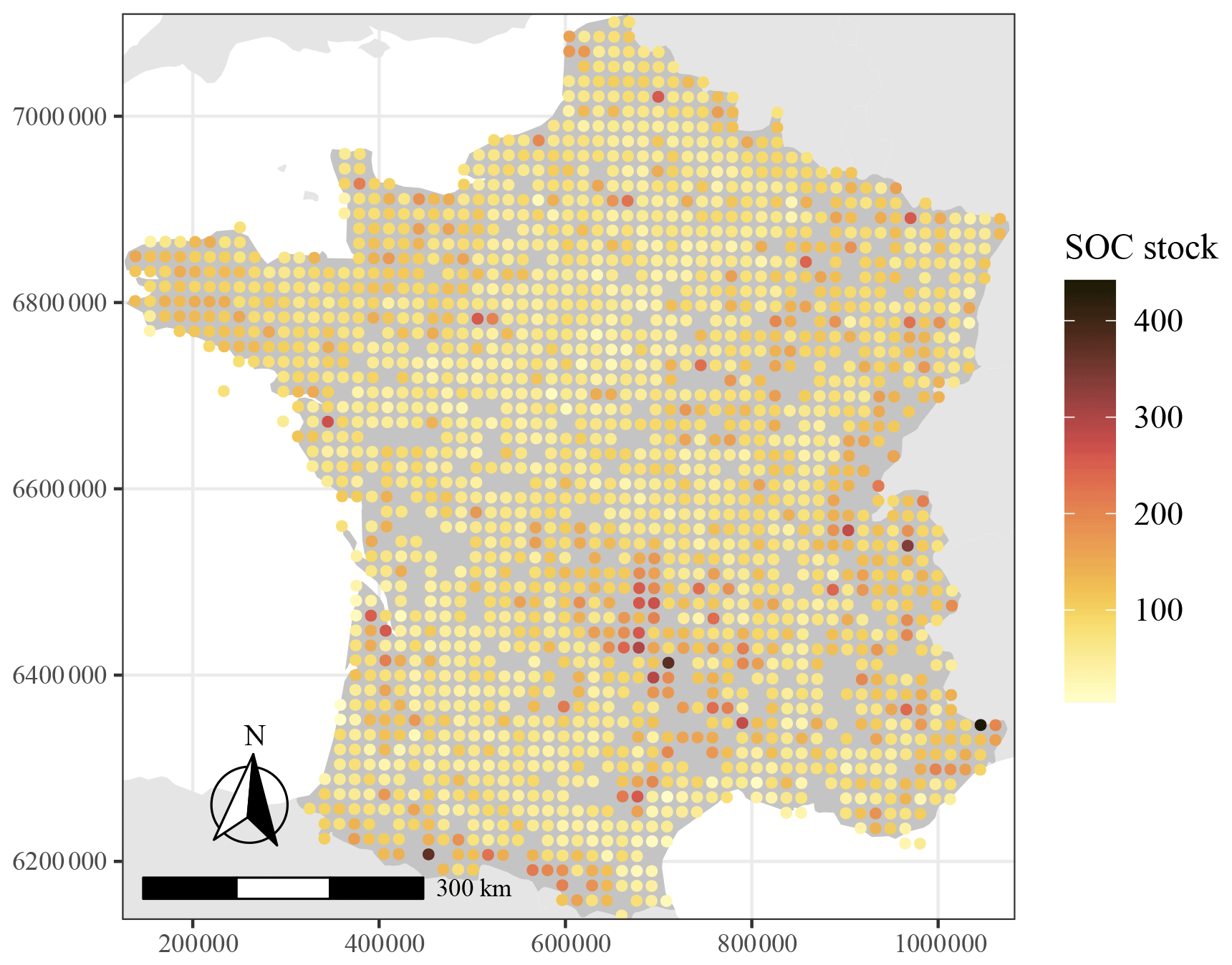
Figure 1 Location of the soil organic carbon stock data (in t ha⁻¹) for mainland France.

2.4 Exhaustive explanatory variables

We use a set of 23 publicly available spatially continuous environmental covariates. The covariates provide information on the main biotic and abiotic factors which are known to affect SOC stocks. The main sources of covariates were the database from BioClim, SoilGrids and a Shuttle Radar Topography Mission (SRTM) elevation model with derivatives. We also used MODIS products from which the normalized different vegetation index (NDVI) map was calculated from the NIR and red spectral bands and a high-resolution land-cover map with seven classes obtained by Sentinel-2 images. Covariates were further grouped into six categories representing (1) the average climate condition, (2) climate seasonality, (3) extreme climate conditions, (4) topography and terrain derivatives, (5) soil properties, and (6) organisms/vegetation. A list of factors and covariates, along with their units and references, is provided in Table 1.

Fick and Hijmans (2017)Fick and Hijmans (2017)Zomer et al. (2008)Fick and Hijmans (2017)Fick and Hijmans (2017)Fick and Hijmans (2017)Fick and Hijmans (2017)Fick and Hijmans (2017)Fick and Hijmans (2017)Fick and Hijmans (2017)Fick and Hijmans (2017)Trabucco et al. (2008)Rabus et al. (2003)Yamazaki et al. (2017)Yamazaki et al. (2017)Yamazaki et al. (2017)Pelletier et al. (2016)Hengl and Gupta (2019)Hengl and Gupta (2019)Poggio et al. (2021)Poggio et al. (2021)Tuanmu and Jetz (2015)Running and Zhao (2019)Lyapustin et al. (2018)Thierion et al. (2018)

Table 1 List of environmental covariates used as predictors in the random forest model with units and associated references when applicable. Covariates are grouped into categories representing average climate conditions, climate seasonality, extreme climate conditions, topography, soil and organisms/vegetation. Covariates have the coordinate system Lambert-93 (EPSG:2154) and the following extent: 6028362–7141392^∘ S, 16877.61–1251060^∘ E.

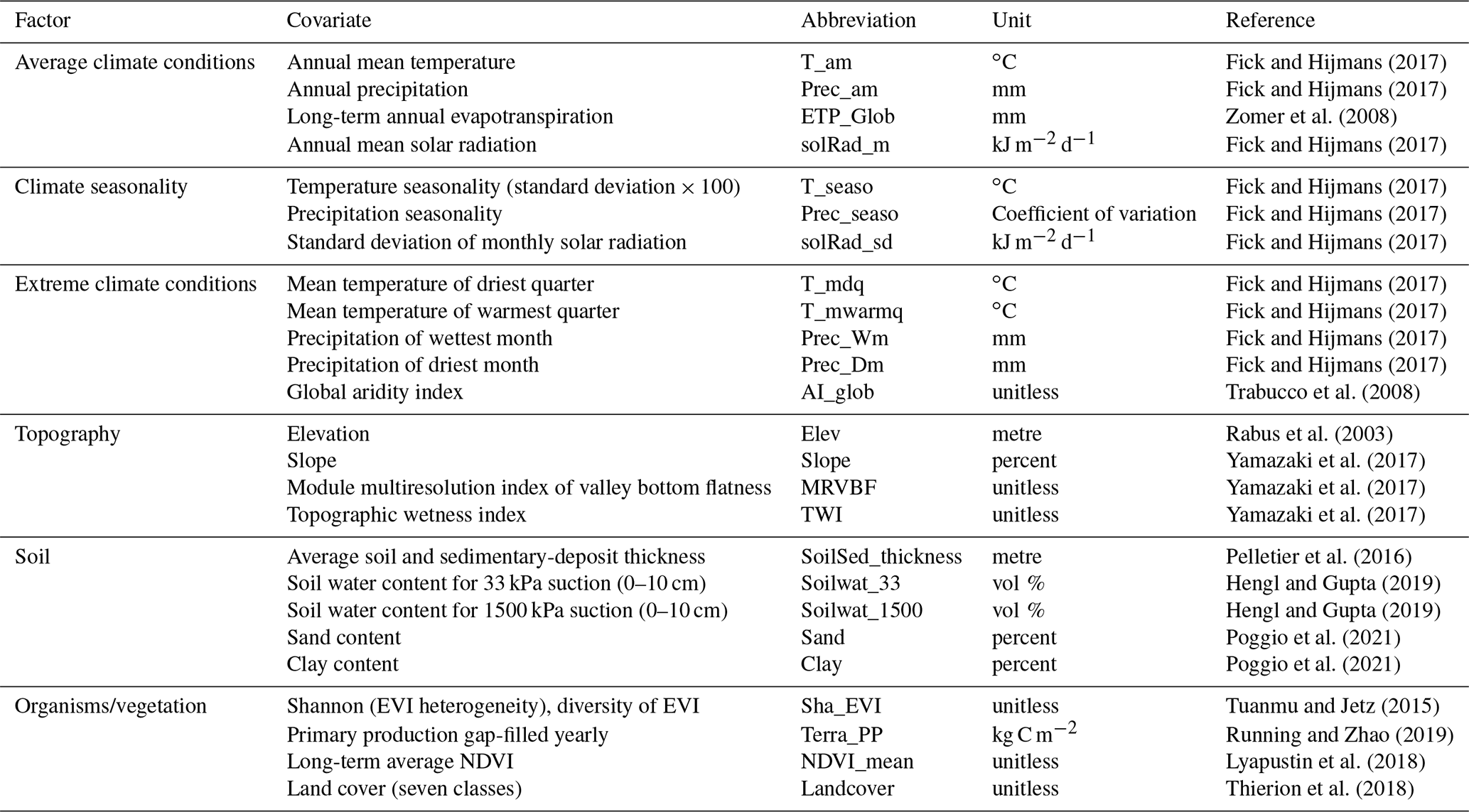
The original covariate resolution spanned from grid cell sizes of 90 m × 90 m to 1 km × 1 km, which we transformed into a common resolution with grid cells of 250 m × 250 m by either resampling with bilinear interpolation or aggregation. Covariates were then converted to the coordinate system Lambert-93 and transformed into a common extent.

2.5 Modelling and mapping of SOC stocks

The SOC stock data and their matching values of environmental covariates were used to build a regression matrix. The modelling approach to establish the relationship between the SOC stocks and environmental covariates is based on random forests.

A random forest (RF; Breiman, 2001) is an ensemble machine learning algorithm based on decision trees. A single decision tree is fitted by partitioning the covariate values of the calibration dataset. Partitions are evaluated based on a splitting metric, and the partition providing the optimal value of the metric is selected. This procedure is repeated until a user-defined value of the node size is reached. The prediction value of a single tree is taken as the average prediction of all nodes at the terminal leaf. In RF, an additional procedure of bootstrapping and aggregating is introduced, where a user-defined number of trees are built from bootstrap samples of the calibration data. In each tree, a random perturbation is further introduced where only a subset of the covariates are used for fitting the tree. The final prediction from a RF model is the average of all the decision trees. The theory of RF has been extensively described in the literature, and we refer the reader to standard textbooks for more details (e.g. Hastie et al., 2009).

Modelling and mapping of SOC stocks with RF are performed with a standard procedure in three steps: (i) model parameter selection, (ii) model fitting and validation, and (iii) prediction. We optimized three parameters: the number of trees, the minimum number of observations in the terminal node and the number of covariates drawn randomly from the covariate set at each split. In the machine learning literature, these parameters are usually denoted ntree, node.size and mtry, respectively. We used the model-based optimization procedure described in Probst et al. (2019) using the mean square error of the out-of-bag prediction as the objective function and 500 iterations. The optimal parameters were ntree =500, node.size =12 and mtry =10. All other parameters were held to their default value.

The performance of the model with optimized parameters was evaluated using a standard random 10-fold cross-validation strategy. The dataset was randomly split into 10 folds of approximately equal size, where 9 folds were used to calibrate the RF model and the remaining fold was left apart for validation. This procedure was repeated 10 times, each time setting aside a single fold. The independent observed values and those predicted by the RF model are used to compute the usual validation statistics. The predictions did not show systematic over- or under-prediction (mean error (ME) was close to 0) and had a root mean square error of 36.4 t ha⁻¹ and a modelling efficiency coefficient (MEC) of 0.31.

The final model for prediction is fitted using all available SOC stock data and the optimized set of RF parameters. Predictions are made for the whole of France at a resolution of 250 m using the spatially exhaustive set of covariates as predictors. This final model along with prediction for the whole of France is used for interpretation with Shapley values.

2.6 Interpretation with Shapley values

The RF model is interpreted with Shapley values (Shapley, 1953), which were described and used in soil science in Wadoux and Molnar (2022). Shapley values were originally developed within coalitional game theory. Consider a game where each covariate is a player and the prediction is the payout; Shapley values distribute the gain to the players (i.e. covariates) according to their relative participation in the outcome. The gain is the prediction for a particular unit minus the average prediction, and the players are the covariates that contribute to the prediction and “collaborate” to receive a gain.

In statistical terms, let a set of covariates of size p be defined by 𝒮 and $\mathcal{S}\backslash \mathit{\{}\mathrm{1},\mathrm{\dots },p\mathit{\}}\setminus \mathit{\left\{}j\mathit{\right\}}$ be a subset of covariates which excludes covariate j. The Shapley value ϕ_0,j for covariate j for a spatial location composed of the vector of covariates x₀ is given by

$$\begin{array}{}\text{(2)}& \begin{array}{rl}{\mathit{\varphi }}_{\mathrm{0},j}=& \sum _{\mathcal{S}\subseteq \mathit{\{}\mathrm{1},\mathrm{\dots },p\mathit{\}}\backslash \mathit{\left\{}j\mathit{\right\}}}{\displaystyle \frac{\left|\mathcal{S}\right|\mathrm{!}\left(p-\left|\mathcal{S}\right|-\mathrm{1}\right)\mathrm{!}}{p\mathrm{!}}}\\ & \left({\widehat{f}}^{*}\left({\mathit{x}}_{i,\mathcal{S}\cup \mathit{\left\{}j\mathit{\right\}}}\right)-{\widehat{f}}^{*}\left({\mathit{x}}_{i,\mathcal{S}}\right)\right),\end{array}\end{array}$$

where $\left|\mathcal{S}\right|$ is the size of the subset which excludes the jth covariate, 𝒮∪{j} is the subset 𝒮 with the jth covariate added, and ${\widehat{f}}^{*}\left({\mathit{x}}_{i,\mathcal{S}}\right)={\mathrm{E}}_{{\mathbf{X}}_{\mathcal{C}}}\left[\widehat{f}\right({\mathit{x}}_{i,\mathcal{S}},{\mathbf{X}}_{\mathcal{C}}\left)\right]$ is the prediction function where covariates not contained in 𝒮 are marginalized (similarly to 𝒮∪{j}). The calibrated RF model is defined by $\widehat{f}$, and X is the matrix containing the covariates from the calibration dataset; X_𝒞 is a subset of covariates where 𝒞 represents the set of covariates not included in 𝒮. Note that ${\widehat{f}}^{*}\left({\mathit{x}}_{i,\mathcal{S}\cup \mathit{\left\{}j\mathit{\right\}}}\right)-{\widehat{f}}^{*}\left({\mathit{x}}_{i,\mathcal{S}}\right)$ can be interpreted as a marginal contribution to the prediction when adding covariate j to the subset of covariates 𝒮. Equation (2) has two components: the first is the marginal contribution for a subset of covariates, whereas the second is a weighted average, giving equal weight to each of marginal contributions of all possible subsets of covariates. The contribution of a covariate to the prediction of a single spatial location is then given by ϕ_0,j.

Calculating the exact solution for Eq. (2) is computationally intractable because it requires estimating the sum of the marginal contribution for a 2^p−1 combination of covariates. To solve this, we use the approximation algorithm developed by Štrumbelj and Kononenko (2014) and based on Monte Carlo sampling. In Štrumbelj and Kononenko (2014), the covariate effect is approximated by integrating over the observations of the calibration dataset. We refer to Štrumbelj and Kononenko (2014) and Molnar (2020, chap. 9) for more detail on the approximation algorithm.

A Shapley value should be interpreted as the contribution of a covariate to the difference between the prediction and the average prediction. One advantage of Shapley values is the set of mathematical axioms from which they are derived, which provide the basis for a rigorous interpretation of their meaning. Further, Shapley values are additive and symmetric: the individual contribution of a covariate to a spatial location can be averaged over a region or a dataset. We give three example uses in the next paragraph.

A Shapley value can be obtained for any single value of the calibration dataset and any prediction at an unobserved location, in the unit of the prediction (e.g. the soil property of interest). They are usually used to evaluate the individual contribution of a covariate to the prediction of a single location (i.e. to perform a local interpretation of the model). Hereafter we describe three uses of the Shapley values for both local and global interpretation.

• Average contribution. Absolute Shapley values can be summed over the individual observations from the calibration dataset to obtain an overall variable contribution to the prediction. Note that while it is similar to the variable importance plot obtained by permutation and often reported in soil modelling studies with machine learning, the average contribution plot has a different interpretation because it is not based on a decrease in model accuracy (unlike permutation plots).

• Partial dependence. A scatterplot of the average of the Shapley values in the calibration dataset against the value of a single covariate gives an indication of the functional form of the association between the soil property and the covariate (i.e. the partial dependence; Hastie et al., 2009). To ease visualization, the individual dots in the scatterplot are fitted with a smooth curve.

• Local and spatial evaluation. The local contribution of the covariate to the prediction is obtained by Shapley values and can be used to generate a spatial pattern. This pattern can in turn be used to obtain the average contribution for areas, such as bioclimatic regions or soilscapes, or for an individual pedon. This approach is computationally very intensive as it requires estimating Shapley values for all spatial locations (discretized into a finite number of grid cells) in the area of interest.

2.7 Practical implementation and computational aspects

The framework for mapping used in this study follows the usual procedure used in digital soil mapping studies; see for example the summary in Hengl et al. (2017, their Fig. 5). In short, SOC stock data obtained at point locations are overlaid with environmental covariates used as predictors to build a regression matrix. This regression matrix is then used to fit and validate the random forest model using 10-fold cross-validation. The final model is fitted using all data and can then be used for spatial prediction using the covariates known exhaustively. Shapley values are estimated on the final fitted RF model using the covariate values and the measured values of SOC stocks. We use the R programming language (R Core Team, 2022) for the SOC stock calculation, covariate pre-processing, model parameter selection, model fitting and prediction, and estimation of the Shapley values. The RF model was fitted using the “ranger” package (Wright and Ziegler, 2017), and the parameter was selected with the tuneRanger function from the “tuneRanger” package (Probst et al., 2019). Estimation of Shapley values was made with the “fastshap” package (Greenwell, 2020). The procedure for estimating the Shapley values spatially was parallelized and combined with a subsampling approach to ease computation. A total of 12 495 098 grid cell locations were taken using a systematic grid sample of 800 000 cells, for which the Shapley values were estimated. We used a number of Monte Carlo samples that was as large as feasible, i.e. 500 in all cases. Calculations were done on an eight-core computer and took approximately 6 d.

3 Results

3.1 Average contribution

Figure 2 shows the magnitude of the covariate contribution to the prediction of SOC stocks averaged over the calibration dataset (average of absolute values in Fig. 2) or for each individual point of the calibration dataset (Fig. 2). Figure 2b indicates that elevation is on average the most important covariate contributing to the prediction of the SOC stocks. NDVI, the mean temperature of the warmest quarter and the annual mean temperature also make a relatively important contribution to the prediction with an average absolute value of nearly 4.3, 4 and 3 t ha⁻¹. Figure 2b further shows that the four most important covariates have a wide range of Shapley values. Elevation, for example, has values between of −10 and 55 t ha⁻¹. The colour scale in Fig. 2b also shows that large positive Shapley values for the elevation covariate are obtained for high elevation, whereas a negative contribution of this covariate to the prediction is obtained for low values of elevation. Other covariates have a similar pattern. For example, while the soil and sedimentary-deposit thickness covariate (SoilSed_thickness) makes a small contribution to the prediction (i.e. the average value in Fig. 2a is 0.7 t ha⁻¹), large values of soil and sedimentary-deposit thickness make a strong positive contribution to the prediction of the SOC stocks.

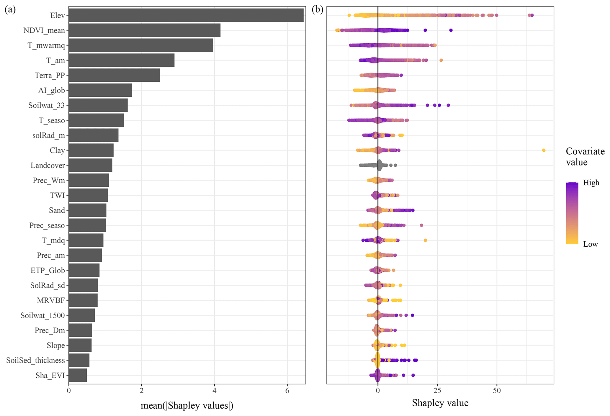
Figure 2 Magnitude of the covariate contribution to the prediction of SOC stocks in France. Plot (a) shows the absolute Shapley values averaged over the calibration dataset, whereas plot (b) shows the Shapley values for each individual point in the calibration dataset, i.e. the contribution of the covariate to the prediction of the SOC stock at that location. The colour scale represents the covariate value normalized in the range [0, 1]. Note that plot (a) is the average of the absolute values presented in plot (b).

3.2 Partial dependence

Figure 3 shows the relative covariate contribution to the individual SOC stock observations of the calibration dataset as a function of covariate values. The four most important covariates of Fig. 2 contributing to the predictions have a well-defined pattern. The covariate contribution to the SOC stock prediction tend to increase with elevation and temperature for values up to 1800 m and 5 ^∘C, respectively, but sharply decreases for higher annual mean temperature or levels off for higher elevation. For high annual mean temperature (i.e. above 10 ^∘C), the Shapley values are negative, which means that the covariate contributes negatively to the SOC stock prediction of these observations. Covariate mean temperature of warmest quarter has a very similar pattern as covariate mean annual temperature. Covariate NDVI contributes negatively to the SOC stock prediction for NDVI values up to 0.6, after which Shapley values are positive. Large values of NDVI make a strong positive contribution (i.e. above 10 t ha⁻¹) to the prediction of SOC stocks. Shapley values of land cover are nearly always positive for six out of the seven classes but nearly always negative for the annual-crop class.

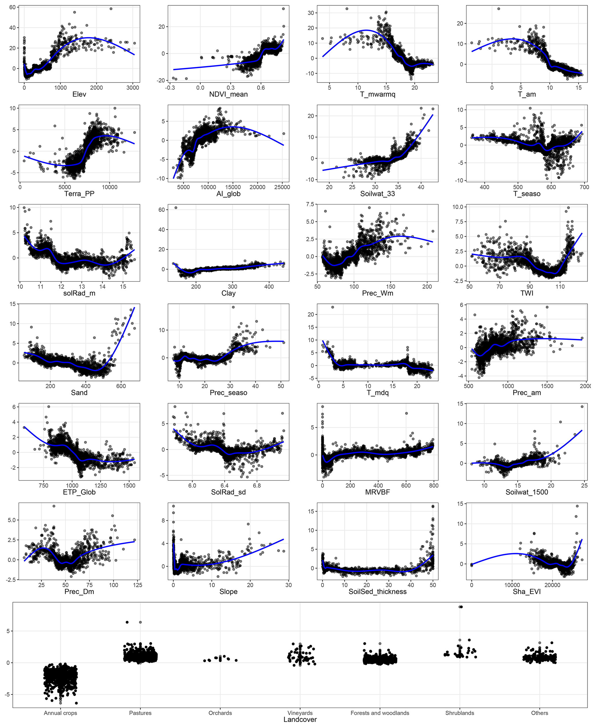
Figure 3 Relative covariate contribution to the SOC stock prediction of the calibration dataset. The x axis shows the covariate values and the y axis the Shapley value of the calibration dataset for this covariate. The blue line is a smoothed curve fitted on the Shapley values for visualization purposes.

3.3 Spatial evaluation

The spatial pattern of Shapley values for the three most important covariates (Fig. 2) is presented in Fig. 4. Note that we present the maps for three covariates but that maps for all covariates are presented in the Supplement (Figs. S1–S3). The three maps presented in Fig. 4 have a smooth and detailed pattern with significant spatial variation. Both elevation and mean annual temperature have a similar pattern of positive contribution in areas of high elevation (e.g. in the Massif Central, the Pyrenees and the Alps mountains), whereas they have negative values in most of south-western France. Elevation also seems to follow the pattern of the two main rivers in the northern part of France, with a noticeable negative contribution of elevation in the streambed. The map of Shapley values estimated for NDVI shows a different spatial pattern with detailed variation. On the southern Mediterranean coast, NDVI has a negative contribution to the SOC stock prediction. An opposite pattern is found on the northern Atlantic coast and in Brittany, where NDVI contributes positively to the SOC stock prediction.

Figure 4 Spatial pattern of the Shapley values over mainland France for the three most important covariates. A dark colour indicates a negative contribution of the covariate to the SOC stock prediction, whereas a bright colour indicates a positive contribution.

Figure 5 is a map of the most important covariates contributing to the SOC stock prediction along with a map showing the proportion of this covariate contribution to the total. To ease visualization, only the five most important covariates are represented. Climate covariates are the most important predictors for nearly all mountainous areas, either T_am in the Massif Central and in the Vosges or T_mwarmq in the Alps and Pyrenees. Vegetation covariates Terra_PP and NDVI_mean are the most important in a large area in the northern part of France and in the extreme east (Terra_PP), whereas NDVI_mean is the most important locally in large patches in Brittany and locally around the Massif Central. Elevation is the most important covariate in the south of the Landes (south-west) and in small areas in Champagne (east of Paris). Figure 5 also shows that the most important covariates contribute between 20 % and 85 % of the total SOC stock prediction but with considerable variation between regions. There is an east–west gradient of decreasing proportion with some local large proportions (e.g. small patches on the Atlantic coast). Large values of proportion are found for all covariates in the Pyrenees and in the Alps and also for small areas in the Massif Central. Small values are found for most of the eastern part of France, with values lower than 0.4, which means that in these areas, the most important covariate shown on the left-hand side of the figure is the most important but contributes a small proportion to the total SOC stock prediction in these areas.

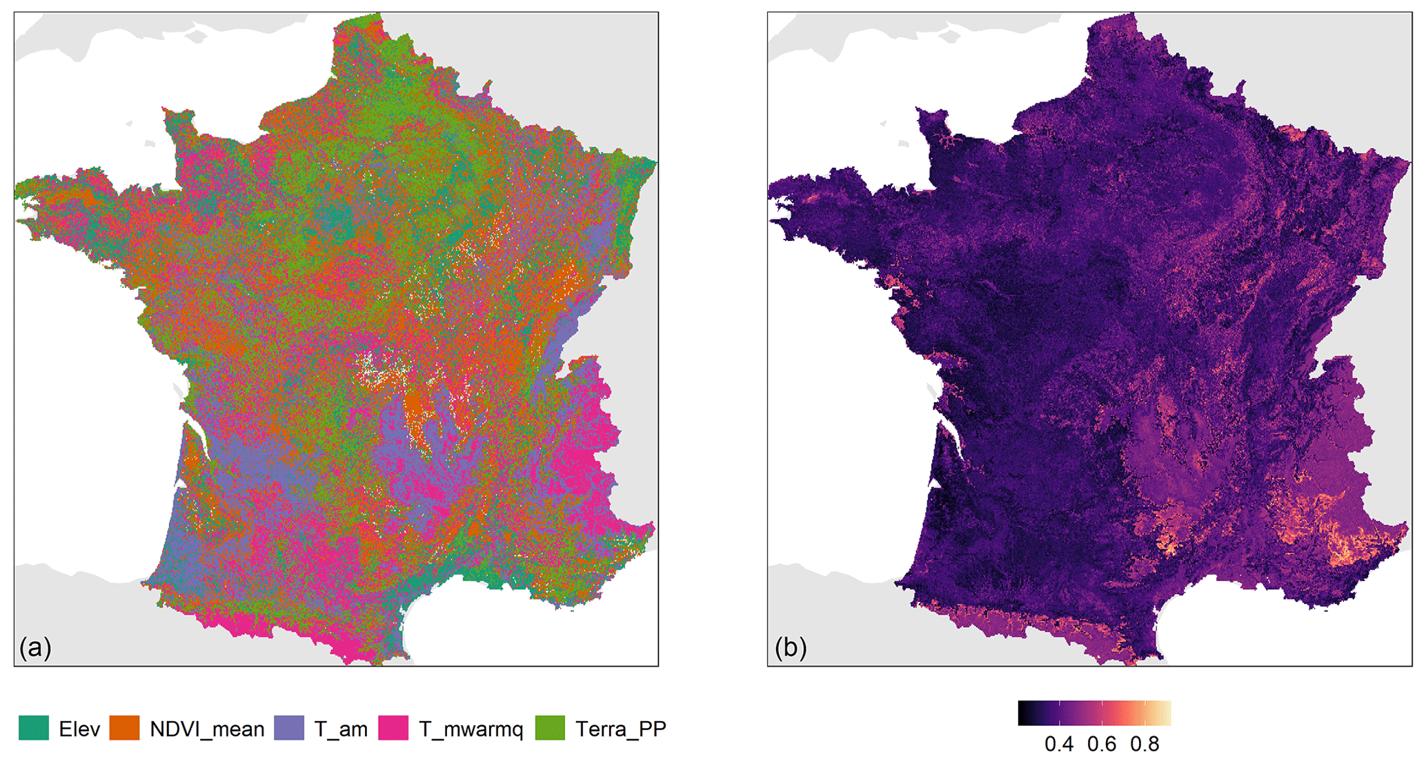
Figure 5 Map of the most important location-specific covariate contributing to the SOC stock prediction (a) for 5 covariates (out of 24) and the proportion of this location-specific covariate relative to the total SOC stock prediction (b).

Figure 6 shows two maps: a map of the most important group of covariates contributing to the SOC stock prediction and a map showing the proportion of this group of covariates relative to the total SOC stock contribution of all groups. The group of covariates related to vegetation is the most important in most parts of France and also shows a high proportion relative to the total (i.e. higher than 0.45). The topography group is the most important in nearly all mountainous areas such as in the Alps, Pyrenees and Massif Central and also forms a relatively high proportion of the contribution to the total SOC stock prediction. The three groups of covariates related to climate seem to not be the most important over large areas but to be important only locally. For example, mean climate condition covariates are important in south-west of France, whereas the group of extreme climate condition covariates is the most important in the eastern part of Brittany. Soil group covariates are the most important in a small area in the north of the Landes where they also contribute to the SOC stock prediction with a proportion of up to 0.5.

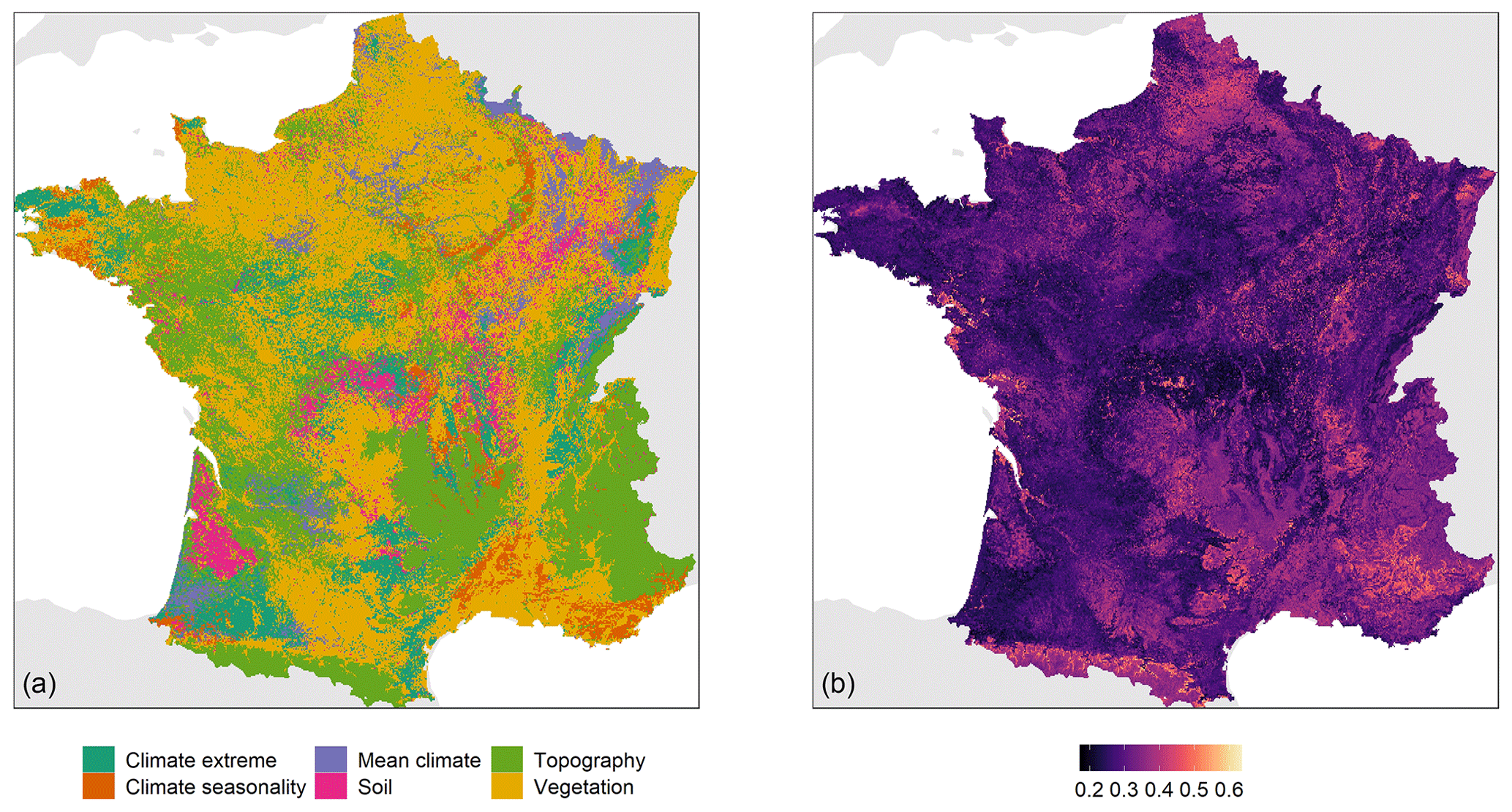
Figure 6 Map of the most important location-specific group of covariates contributing to the SOC stock prediction (a) and proportion of this group relative to the total SOC stock prediction (b).

Using the carbon-landscape zones from Chen et al. (2019), we calculated and report in Fig. 7 the average absolute Shapley value for each group of covariates and for each of the 10 carbon-landscape zones (CLZs). Figure 7 shows that overall some groups of variables are more important than others. For example, vegetation and topography covariates are, for nearly all CLZs, more important (i.e. with larger absolute Shapley values) than other groups such as climate seasonality and soil. Mountainous areas which have higher SOC stocks also have high Shapley values for mean and extreme climate conditions, but the highest values are found for topography. Vegetation is relatively important in nearly all CLZs and is the most important for the CLZs corresponding to areas in a large part of southern France.

Figure 7 Maps of the most important group contributing to the SOC stock prediction for the 10 carbon-landscape zones of mainland France. Values are absolute Shapley values averaged spatially by carbon-landscape zone.

3.4 Local evaluation

Figure 8 shows the contribution (i.e. the Shapley values) of the covariates to the SOC stock prediction at two spatial locations in (a) a forested area in the Landes (south-western France) and in (b) an agricultural area of Champagne (north-eastern France). The two locations have predicted SOC stock of 98 and 92 t ha⁻¹, respectively. There is large difference in the estimates of Shapley values between the two locations. For the Landes, the soil and sedimentary thickness covariate is the main positive contributor (8.3 t ha⁻¹) to the SOC stock prediction, followed by NDVI_mean, Terra_PP and sand. The two main negative contributors are Elev and T_mwarmq. A very different pattern is observed for the Shapley values in Champagne, where T_am is the main positive contributor, whereas the land-cover class annual crops is the main negative contributor with a value of −4.9 t ha⁻¹. The variables NDVI_mean and Terra_PP are also major negative contributors.

Figure 8 Contribution of the covariates to the SOC stock prediction at two spatial locations in (a) a forested area in the Landes (south-western France) and in (b) an agricultural area of Champagne (north-eastern France). Both locations have a close range of predicted values of SOC stocks of around 95 t ha⁻¹. The blue colour indicates a positive contribution of the covariate to the SOC stock prediction, whereas a red colour indicates a negative contribution. The y axis shows the covariate value for the prediction at the location. Satellite images from © Google Maps (2022, CNES/Airbus, Maxar Technologies, available through https://www.google.com/maps/, last access: 2 July 2022).

4 Discussion

4.1 Modelling and mapping of SOC stocks

The validation statistics obtained by the RF model were in good agreement with previously published studies, although it is generally difficult to draw conclusions on the quality of the fitted RF model compared to other studies mapping SOC concentration or density. The MEC obtained in our study is within the upper range of the R² values for large-area mapping of SOC reported in Minasny et al. (2013). When mapping SOC stocks over large areas, differences in model performance can arise from whether the bulk density is measured or estimated and from the covariate set used to fit the model. Other causes of difference are the modelling procedure and the validation strategy (e.g. (spatial) cross-validation, independent validation with probability sampling), which can both have a substantial impact on the resulting map quality. Our fitted RF model had no bias and a MEC of 0.31. This is similar to previous studies on mapping SOC stock for large areas. For example, Martin et al. (2014) fitted a boosted regression tree model on a similar set of the RMQS sampling sites in France and obtained an R² of 0.36 and negligible bias, whereas Mishra et al. (2009) obtained a ME and R² of −0.1 and 0.46, respectively, for mapping SOC stocks in the state of Indiana (USA). Also, Lacoste et al. (2014) reported an R² of 0.43 for modelling SOC stocks in the O horizon of the French forest soils. The spatial pattern of the SOC stock map for the 0–50 cm depth intervals (not shown) obtained by prediction with the RF model also agreed with past studies. Studies by Martin et al. (2011, 2014) reported similar patterns of SOC stocks in France for the 0–30 cm depth interval. The later study of Martin et al. (2014) performed a rigorous validation assessment of several modelling approaches to SOC stocks in France, from which we found no systematic difference with the maps made in this study or with the error maps made in Martin et al. (2011) or Meersmans et al. (2012). Overall, the validation statistics and spatial pattern of prediction by the RF model suggest that the RF fitted in this study is sufficiently accurate to serve as a basis for the interpretation with Shapley values.

4.2 What did Shapley values reveal about the drivers of SOC stocks in mainland France?

The Shapley values revealed that the covariate contribution to the SOC stock prediction varied greatly among spatial locations and between CLZs. The results suggest relationships between environmental covariates and SOC stocks which have been abundantly documented in the literature and other relationships that may highlight the limitations of empirical modelling for the SOC stock prediction. Hereafter we describe how the group of covariates relates to potential acting processes of soil carbon storage and how the Shapley values revealed potential limitations of the empirical modelling of SOC stocks.

4.2.1 Climate

The effect of climate on SOC stocks, here through the temperature and precipitation variables (i.e. T_am and P_am), is usually linked to a number of soil carbon decomposition processes as well as plant growth. In our case, covariates related to temperature (i.e. T_am, T_mwarmq and T_mdq) were the most important average contributors to the SOC stock prediction, but the pattern reported in Figs. 2 and 3 shows that the relationship with SOC is complex (i.e. non-monotonic, non-linear and with strong discontinuities). In fact, temperature is one of the most important climate drivers affecting SOC mineralization while at the same time also affecting net primary productivity (Martin et al., 2011). Here, after a certain threshold (i.e. 6 ^∘C), the relationship between SOC and temperature decreases, likely because of the combined effects of the negative impact of extreme temperatures on plant productivity and their positive effect on SOC mineralization. The impact of temperature is also exemplified in the CLZs related to high SOC stocks in mountainous areas (Fig. 7); the group of climate covariates makes the most important contribution, which may be caused by the low-mineralization processes due to cold temperature. Figure 9 illustrates the combined effect of mean temperature and NDVI on SOC stocks. Optimum conditions in term of SOC stocks correspond to high NDVI mean levels (around 0.75) and moderate temperature (hence mineralization) close to 7.5 ^∘C on average. Similar optimal conditions are found for lower NDVI levels but where low temperature enables slow turnover of soil organic matter (SOM).

This relationship is also modulated locally by the extreme climate condition, which acts as a limiting factor in carbon storage (Reichstein et al., 2013). Indeed, Fig. 8 shows that T_mwarmq importance is overall greater than the importance of T_am, and Fig. 3 shows that variations in SOC stocks induced by T_mwarmq are greater than variations in T_am. The shape of the relationship between T_mwarmq and SOC stocks is close to that of T_am and SOC. This might be because, overall, similar (and possibly opposing) processes relating temperature to both plant productivity and SOM mineralization come into play. Also, for T_mdq above 19 ^∘C, SOC stocks remain constant. To our knowledge there is no best explanation, but there is a probable correlation with other variables, such as land use, or other climate variables including precipitation. Typically in areas with a very hot summer, drought possibly also limits SOM mineralization, avoiding temperature increases to further facilitate SOC stock depletion.

4.2.2 Topography

Topographic covariates control many of the redistribution processes influencing SOC stocks. In our study case, elevation was on average the most important covariate for explaining the SOC stock variation, with a trend (Figs. 2 and 3) of increasing Shapley values for higher elevation (i.e. elevation contributes positively to the SOC stock prediction). In fact, the higher SOC stocks in France are found in the mountainous areas of the Pyrenees, Massif Central and Alps. This is an expected finding already reported in the literature for various ecosystems (e.g. by Lemenih and Itanna, 2004) and which is usually attributed to the combined effect of temperature and precipitation (Saby et al., 2008). In our study, the Shapley values revealed that the effect of elevation is merely related to its relationship with temperature; see, for example, the inverse relationship between these two variables in Fig. 3. The slope covariate had overall a positive effect on SOC stock prediction (Fig. 2), but the maps of slope in the Supplement (Fig. S3) show that this occurs both in mountainous areas (e.g. the Alps) and in river streambeds (e.g. the Seine River stream). The effect of slope on SOC stocks is logical in this study case and has already been reported elsewhere (e.g. Stevens et al., 2014). However, in Stevens et al. (2014) the relationship between slope and SOC stocks is negative. This suggests that in our case the positive effect of slope might be due to the location of steep slopes, i.e. mostly in mountainous areas. Higher SOC stocks with steeper slopes might also result from the combined effect of orientation and resulting effects on moisture and temperature.

4.2.3 Soil

Soil clay has a well-known effect on SOC stock through physical interaction and protection of organic matter from decomposition (Stewart et al., 2008). We found that prediction of SOC stocks monotonically increased with higher values of clay, which is consistent with previous studies on the same area (e.g. Martin et al., 2011). The soil water regime made a relatively moderate contribution to the SOC stocks, but this was very contrasted locally for the Soilwat_ covariate. For example, large agricultural and semi-mountainous areas from the centre to north-west of France had a positive Shapley value for this covariate (see also the Supplement, Figs. S1–S3). For these areas there might be a contribution of processes relying on soil moisture for SOC storage, such as soil carbon mineralization by microbes (Orchard and Cook, 1983). From the available results, however, it is disputable to draw conclusions on this process. We also found that the soil covariate SoilSed_thickness, which represents the soil thickness to the unweathered bedrock, was not an important contributor on average but that for the deep sandy soils of the Landes, this variable was a very important predictor of the SOC stocks. In this regard, the sand covariate was an important factor contributing to SOC stock prediction in the Landes because in these areas the SOC stocks are mainly characterized by acidic sandy soils that were undisturbed for a long time by agriculture. The high SOC stocks in these areas, however, are not due to the sandy soils but due to the combined effect of land use and carbon input (see below). It is likely that the empirical model of SOC stocks predicts high values in these areas for the wrong reasons.

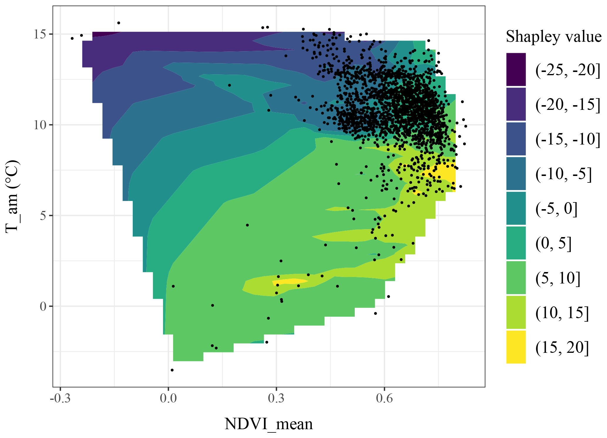
Figure 9 Two-dimensional visualization of NDVI_mean and T_am contributions to the SOC stock prediction. Black dots indicate a point in the calibration dataset. The colour represents the Shapley values. The surface was obtained by linear interpolation of the Shapley values obtained from the calibration dataset.

4.2.4 Organisms/vegetation

Both NDVI_mean and Terra_PP were important covariates for predicting the SOC stocks not only on average (Fig. 2) but also locally in many parts of France (Figs. 5 and 6). SOC stocks are mediated by a balance of net C input and net loss, and vegetation acts on SOC stocks through C inputs. This is shown in Fig. 4 where the map of Shapley values for NDVI_mean has high values in large forested areas. Land use also has an important effect on SOC stocks over time. In Fig. 3 it is shown that six out of seven categories make a positive contribution to the SOC stock prediction but that for annual crops the contribution was nearly always negative. This is a realistic result that has been reported abundantly in the literature as arable land cropping systems are characterized by large human appropriation of the net primary productivity (Plutzar et al., 2016). In the Mediterranean CLZs, conversely, NDVI and Terra_PP covariates were not important. In Mediterranean areas, carbon storage is mitigated by land use and mediated by water availability. We also note the stepped pattern of the NDVI_mean covariates in the SOC stock prediction shown in Fig. 3. This suggests that NDVI compensates for a missing carbon input covariate or an insufficient number of land-use classes. In our case the Shapley values reveal that the covariates are not sufficiently precise or that potential covariates are missing to predict the SOC stocks. For example, mitigation occurs by land use between NDVI and the carbon input.

Finally, the Shapley values presented for two spatial locations in Fig. 8 reveal a well-known relationship of SOC stocks with their environment. In the Landes the SOC stock is relatively high because despite sandy acid soils that do not store the carbon well, the system is stable over time with no cultivation and a land use of pine forest. The Landes is also characterized by Podzols with accumulation horizons which are likely to contain more SOC in the subsoil. This is reflected in the Shapley values: the soil thickness and sand content are important predictors of the SOC stocks, as well as vegetation. This is counter-intuitive, and this suggests that the model did not capture well the land-use information or that we did not have sufficient land-use classes to discriminate historical land use. The spatial location in Champagne, conversely, is within an area with relatively high clay content (high physical protection), and low temperature reduces carbon mineralization in cold winters. It is therefore no surprise that the two most important variables contributing to the SOC stocks in this location are temperature and clay content but that this was strongly mitigated by the land-use class.

4.3 Comparison with previous studies

We found no notable difference in results with previous studies investigating the controlling factors of SOC (Arrouays et al., 2001) and SOC stock variation in France (e.g. Martin et al., 2011; Mulder et al., 2015). In these studies too, the authors concluded that land use or vegetation, soil physical and chemical properties, and climate had the most important effect on SOC levels. In our case, we had a different set of explanatory variables and we investigated the controlling factors for a single depth interval (i.e. 0–50 cm). In spite of these differences, we also found the climate and vegetation were major factors contributing to the SOC stock prediction. The reported effect of clay and soil water regime is the same as reported in Martin et al. (2011), but they also reported that rainfall was consistently the most important predictor, whereas in our case temperature was the most important. The effect of these two variables on SOC storage is dependent on many factors (e.g. chemical protection, freezing, plant productivity), which may be accounted for by a different set of covariates. Both precipitation and temperature as important predictors are plausible outcomes of the modelling, but more thorough analysis is need to investigate this. In Mulder et al. (2015), it was found that evapotranspiration, net primary productivity and clay content were important predictors, for both topsoil and subsoils. They too found that the influence of environmental factors varied greatly among soil-landscape zones.

4.4 Limitations of Shapley values and the interpretation of complex models

The results appear realistic, both in relation to the existing known soil carbon storage processes and with regards to previous studies in the same area. One must take care however when interpreting Shapley values as potential causal mechanisms describing the spatial pattern of SOC stocks. Despite selecting a set of covariates that were intended to represent underlying mechanisms involved in SOC storage, these are only proxy variables and do not necessarily relate to processes involved in SOC stock variation. Several studies have argued in this sense (e.g. Wadoux et al., 2020). In this work we limited our analysis of the Shapley values to the connection of the relationship found between environmental covariates and SOC stocks to possible processes involved in soil carbon decomposition and storage, but we did not proceed any further in assuming that we inferred causal conclusions from these values. Doing so would require additional experiments and a more thorough analysis. Another aspect to be considered when interpreting Shapley values from the derived relationships between covariates and the response variable is the accuracy of the covariates. This is particularly important when using the covariate rankings provided by Shapley values. We also stress that the present-day SOC stocks are the outcome of the integrated effect of processes over time, which for SOC can last decades to centuries. The covariates that we used only reflect the current situation and do not represent past processes well (e.g. climate or land use). This may also affect the model accuracy and limit the interpretation of the relationships reported in this study.

An interesting and novel aspect of the use of Shapley values is the possibility of understanding whether the complex model is predicting for the right reasons. Empirical models used in soil mapping studies include little or no pedological knowledge on the property of interest. Instead the models search for correlation among the data and predict using empirical rules. Often these models are more accurate than simple models (i.e. linear regression), but it is unclear whether they are able to predict because of spurious associations between data or through a correlation that has an underlying causal structure (Wadoux et al., 2021b, Sect. 5.2). In our study, the Shapley values revealed that in the Landes, for example, SOC stocks were accurately predicted but that the model used the correlation with the sand to predict these high values, instead of the expected historical land use and carbon input information. An obvious solution to this problem is to obtain better covariates and more covariates on carbon input and historical land use, which should allow the model to discern better the controlling factor of SOC storage.

Although we used Shapley values to obtain the pattern of controlling factors in a large area, Shapley values require a lot of computing time. In our case computing took approximately 6 d of parallel processing in a standard eight-core desktop computer, but processing time is largely determined by the number of Monte Carlo simulations. We used 500 Monte Carlo simulations, which we considered sufficient. This was tested by a scatterplot of the Shapley values estimated by a number of Monte Carlo simulations against another set of Shapley values estimated by the same number of Monte Carlo simulations. The results (not shown) suggested that any number greater than 100 would provide a sufficiently accurate estimate of the values. Excessive computing time, however, might often preclude the use of Shapley values for continental and global studies. To date, two approaches exist for approximating Shapley values: the one described in Štrumbelj and Kononenko (2014) that we used in this study, and the one described in Lundberg and Lee (2017) called SHAP (see also studies in soil science using SHAP; Padarian et al., 2020; Beucher et al., 2022). The SHAP approach might be valuable too although we did not consider it in our case. SHAP can be viewed as a local approximation of Shapley values and might provide a computationally efficient (near-)exact approximations of Shapley values for specific families of models such as gradient-boosted decision trees. To the best of our knowledge, we are not aware of studies describing the differences between the two approaches and whether they have an impact on the estimated values. This may be investigated further in future works.

5 Conclusions

We introduced and implemented the Shapley values for interpreting a machine learning model. Using the soil organic carbon stocks for the 0–50 cm depth intervals and a large set of environmental covariates as predictors, Shapley values revealed insights into the global and local factors contributing to the SOC stock variation and into how the model adjusted the prediction locally. The main conclusions are as follows:

• Shapley values not only revealed the global contribution of environmental factors to the SOC stock prediction but also enable us to obtain the functional form of this association and a spatial pattern of the covariate contribution to the prediction.

• The covariate contribution for SOC stock prediction varied greatly by spatial location and between carbon-landscape zones.

• The results of the interpretation were valid in light of existing and well-described soil processes acting in soil carbon decomposition in the area.

• In a test of predicting SOC stocks in two spatial locations with similar stock values but very different environments, we obtained Shapley values that show individual covariate contributions to the prediction.

• In our case study, a comparison with existing works investigating the controlling factors of SOC stock variation showed that Shapley values found similar relationships between SOC stocks and environmental factors.

• We need to further test the use of Shapley values on covariates that are more precise (for example, measured at site) and more directly linked to factors conditioning SOC stock variation, for example by using covariates linked to carbon inputs instead of NDVI.

The results and comparison with existing studies suggest that Shapley values are a useful tool to give insight about the controlling factors of SOC stock variation, both globally and locally for specific spatial locations. We conclude that Shapley values comprise a promising tool to interpret complex models and that their main added value is to enable a local interpretation of the environmental factors contributing to a prediction.