Spatial prediction of organic carbon in German agricultural topsoil using machine learning algorithms

As the largest terrestrial carbon pool, soil organic carbon (SOC) has the potential to influence and mitigate climate change; thus, SOC monitoring is of high importance in the frameworks of various international treaties. Therefore, high-resolution SOC maps are required. Machine learning (ML) offers new opportunities to develop these maps due to its ability to data mine large datasets. The aim of this study was to apply three algorithms commonly used in digital soil mapping – random forest (RF), boosted regression trees (BRT), and support vector machine for regression (SVR) – on the first German agricultural soil inventory to model the agricultural topsoil (0–30 cm) SOC content and develop a two-model approach to address the high variability in SOC in German agricultural soils. Model performance is often limited by the size and quality of the soil dataset available for calibration and validation. Therefore, the impact of enlarging the training dataset was tested by including data from the European Land Use/Cover Area frame Survey for agricultural sites in Germany. Nested cross-validation was implemented for model evaluation and parameter tuning. Grid search and the differential evolution algorithm were also applied to ensure that each algorithm was appropriately tuned . The SOC content of the German agricultural soil inventory was highly variable, ranging from 4 to 480 g kg⁻¹. However, only 4 % of all soils contained more than 87 g kg⁻¹ SOC and were considered organic or degraded organic soils. The results showed that SVR produced the best performance, with a root-mean-square error (RMSE) of 32 g kg⁻¹ when the algorithms were trained on the full dataset. However, the average RMSE of all algorithms decreased by 34 % when mineral and organic soils were modelled separately, with the best result from SVR presenting an RMSE of 21 g kg⁻¹. The model performance was enhanced by up to 1 % for mineral soils and by up to 2 % for organic soils. Despite the ability of machine learning algorithms, in general, and SVR, in particular, to model SOC on a national scale, the study showed that the most important aspect for improving the model performance was to separate the modelling of mineral and organic soils.

1 Introduction

Soil organic carbon (SOC) is the largest terrestrial carbon pool (Wang et al., 2020) and plays an essential role in agriculture. As SOC influences various physical, chemical, and biological properties of soil (Reeves, 1997), numerous studies recognise it as a crucial indicator of soil quality (Castaldi et al., 2019; Meersmans et al., 2012a; Reeves, 1997); therefore, its decline is identified as a threat that leads to soil degradation (Castaldi et al., 2019; Poeplau et al., 2020a). Moreover, when considering carbon sequestration, the SOC pool provides the option for climate change mitigation (Meersmans et al., 2012a; Ward et al., 2019). Thus, SOC monitoring is important in the frameworks of various international treaties, such as the European Union Soil Thematic Strategy and the United Nations Framework Convention on Climate Change (Meersmans et al., 2012b; Poeplau et al., 2020a), and there is growing interest in understanding the spatial distribution of SOC at different scales in response to the increasing demand for a better assessment of SOC (Minasny et al., 2013). This is particularly important for agricultural land due to its potential for carbon sequestration (Lal, 2004).

In digital soil mapping (DSM), a soil attribute is described by an empirical quantitative function of seven factors: soil properties, climate, organisms, topography, parent material, time, and spatial position (McBratney et al., 2003). This function, known as the SCORPAN model, can be applied to spatially predict the soil property of interest (Minasny et al., 2013). Within this framework, machine learning algorithms aim to automatically extract information from the data for predictive purposes (Behrens et al., 2005). This is of particular interest in view of the recent expansion of soil databases and the vast amount of data available to approximate the soil forming factors (McBratney et al., 2003; Wadoux et al., 2020), thereby making DSM cost-effective, time-efficient, and applicable over large areas with good results (Behrens and Scholten, 2006; Camera et al., 2017).

Despite the advantages of DSM, it is crucial to note that its application requires soil databases of an adequate sample size for training and testing. Furthermore, consistent and quality-checked datasets are a prerequisite for DSM. Several soil inventories and monitoring networks for SOC have been established on a national scale in countries such as Sweden (Poeplau et al., 2015), France (Belon et al., 2012; Arrouays et al., 2002), Denmark (Taghizadeh-Toosi et al., 2014), and Scotland (Chapman et al., 2013). However, the most critical shortcomings of soil inventories in Germany concern the lack of large-scale, high-quality SOC monitoring (Wiesmeier et al., 2012) with periodic and standardised sampling focused on agricultural soils (Prechtel et al., 2009). These issues have now been addressed in the first German agricultural soil inventory (Poeplau et al., 2020a). This inventory was carried out on a national scale considering a sampling depth of 1 m at 3104 sampling sites covering agricultural land. Furthermore, on the European scale, the Land Use/Cover Area frame Survey (LUCAS), undertaken in 2009, is the first harmonised topsoil survey with physico-chemical analyses of georeferenced topsoil samples from 23 European states (Tóth et al., 2013). Therefore, by taking advantage of DSM and of both the German agricultural soil inventory and the LUCAS survey, it is possible to regionalise from single-point measurements to obtain high-resolution cover soil data nationwide and, thus, provide a baseline for both SOC monitoring and environmental and climatic modelling for Germany.

Boosted regression trees (BRT), random forest (RF), and support vector machine for regression (SVR) are among the most widely used algorithms in DSM (Padarian et al., 2020). For example, Martin et al. (2014) predicted topsoil SOC on a national scale for France using the BRT algorithm by comparing its results when the same algorithm was coupled with a geostatistical approach. The above-mentioned authors concluded that, due to the large distances between sampling sites, spatial autocorrelation is unlikely in most national inventories, and the BRT algorithm alone is sufficient for this purpose. This algorithm has also been used on a national scale in China for data from the 1980s and 2010s in order to predict topsoil SOC and its spatial–temporal change as well as the main drivers of its variability (Wang et al., 2021). RF has also become more popular in DSM due to its relative simplicity and performance. For example, this algorithm was implemented to map topsoil SOC on a national scale in Madagascar and identify its main drivers (Ramifehiarivo et al., 2017). Ramifehiarivo et al. (2017) concluded that the uncertainty of the map generated by RF model training was lower when compared with the maps that had formerly been generated for the country. Moreover, this algorithm was compared with the Cubist algorithm for mapping SOC at different resolutions on a regional scale in China and was found to outperform it (Li et al., 2021). Fewer studies have used SVR than RF to predict SOC. Studies have mainly implemented SVR on a regional scale with a limited number of samples (Forkuor et al., 2017; Were et al., 2015) or on a national scale (Switzerland) with very few samples (150 samples from the European LUCAS survey) (Zhou et al., 2021). However, in a study comparing different algorithms, including SVR and RF, on a continental scale and within each country in Latin America, the results indicated that the algorithm that showed the best performance varied from country to country (Guevara et al., 2018). The difference mainly depended on data density, quality, representativeness, and country size, which affect the heterogeneity of land use and environmental conditions.

Another important consideration when applying machine learning is the impact of the parameter-tuning strategy on algorithm performance. This is particularly crucial when the objective of the study is to compare different machine learning algorithms. Although some algorithms are less sensitive to tuning, this step is more important for others, particularly those with a higher number of parameters (Tziachris et al., 2020; Wadoux et al., 2020). Furthermore, as algorithms differ by parameter type (continuous or discrete), the chosen strategy should be aligned with this difference (Ließ et al., 2021). For example, the performance of SVR and BRT has been shown to be better and more stable when optimised by a differential evolution (DE) algorithm than when tuned by grid search (Zhang et al., 2011; Gebauer et al., 2020). Despite this importance, in a review of studies that have applied DSM, Wadoux et al. (2020) state that almost half of the studies implemented parameter tuning, with grid search being the most common strategy applied for this purpose. This finding indicates that the role of parameter tuning and optimisation is unfortunately undermined in DSM. This is particularly evident when the application of machine learning in this field is compared with other fields, where various studies have shown the impact of parameter-tuning strategies on the performance of algorithms such as SVR and BRT (Liang et al., 2011; Santos et al., 2021; Bhadra et al., 2012; Deng et al., 2019).

Therefore, the aims of the present study were as follows: (i) to address the above-mentioned parameter-tuning issue and, consequently, provide a true comparison of the performance of BRT, RF, and SVR in modelling the SOC content of German agricultural topsoils (0–30 cm); (ii) to assess the impact of the training dataset size by extending the data of the German agricultural soil inventory with LUCAS data for model calibration; and (iii) to develop a two-model approach to address the high variability in SOC in German agricultural soils and compare it with a single-model approach.

2 Materials and methods

2.1 Soil data

The models were built using SOC content data from two soil inventories. The first dataset was from the German agricultural soil inventory, which is comprised of 3104 sites collected along a 8 km × 8 km grid throughout Germany (Poeplau et al., 2020a). The sites were sampled and analysed for different soil properties, including the SOC content measured via dry combustion, for the upper 30 cm of the soil between 2012 and 2018. The second dataset was the European LUCAS survey that provides SOC content, similarly also measured via dry combustion, with the sampling depth limited to 0–20 cm (Tóth et al., 2013). For Germany, data collected on agricultural soils cover 1223 sites. Therefore, in order to harmonise the depths of both datasets, they were subdivided into two classes – mineral and organic soils – according to a SOC threshold value of 87.0 g kg⁻¹. Accordingly, all soils above this threshold were considered to be organic soils, comprising peat soils and disturbed and degraded peat soils (Poeplau et al., 2020a). Linear regression functions were derived for both mineral, Eq. (1), and organic, Eq. (2), soil classes using the data of the German agricultural soil inventory to relate the SOC content of the 0–30 cm data to that of the 0–20 cm data. These functions were then applied to the corresponding soil class from the LUCAS data in order to estimate the 0–30 cm topsoil SOC. The generated 0–30 cm LUCAS data and the original 0–20 cm LUCAS data were then used by each algorithm to check the effect of depth extrapolation.

$$\begin{array}{}\text{(1)}& {\displaystyle }y=\mathrm{1.01}+\mathrm{0.881}x\text{(2)}& {\displaystyle }y=\mathrm{1.6}+\mathrm{1.02}x\end{array}$$

2.2 Covariates

Covariates from multiple sources were included to approximate the SCORPAN factors throughout Germany. In the case of multiple data products for one covariate, the one with the best quality (fewer artefacts) and the highest spatial resolution was added. These were then resampled in ArcGIS (Esri, 2013) using the INSPIRE standard grid at a 100 m resolution (Eurostat grid generation tool for ArcGIS, https://www.efgs.info/information-base/best-practices/tools/eurostat-grid-generation-tool-arcgis/, last access: 10 December 2020). The resampling method was either the nearest-neighbour technique for categorical covariates or the bilinear interpolation technique for continuous covariates. The same INSPIRE grid was also used to rasterise the vector covariates. Finally, they were stacked and overlaid on SOC databases in order to extract values at the sampling points.

Following the SCORPAN framework, 24 covariates including x and y coordinates for spatial position were compiled. In order to represent the climate factor (C factor), precipitation (DWD, 2018c), sunshine duration (DWD, 2017), summer days (DWD, 2018b), and minimum temperature (DWD, 2018a) were applied according to the study of Schneider et al. (2021). Using principal component analysis, these four covariates were identified to be the most important out of 34 available climate factors for SOC in the German agricultural soil inventory dataset. Moreover, the agricultural land use type is one of the main drivers of SOC variability on a national scale (Poeplau et al., 2020a); therefore, the land use map from the official Topographic–Cartographic Information System (BKG, 2019) with its corresponding classes according to the German agricultural soil inventory was rasterised and included. This is a categorical covariate, representing the organism factor of SCORPAN (O factor), which distinguishes croplands from grasslands and captures their spatial distribution throughout Germany.

The Digital Elevation Model over Europe (EU-DEM; European Union Copernicus Land Monitoring Service and EEA, 2016) with an original resolution of 25 m was resampled to 100 m. Six covariates derived from the resampled layer were also added to integrate the relief parameter (R factor). Slope, plan curvature, and profile curvature, generated with the System for Automated Geoscientific Analyses (SAGA; Conrad et al., 2015), were included to capture the slope's gradient, convexity–concavity, and convergence–divergence. These factors influence the soil distribution throughout the landscape (e.g. affecting flow over the surface), thereby impacting SOC and its dynamic (Ritchie et al., 2007). Moreover, slope exposition (aspect) was calculated from the EU-DEM, as it influences soil development and subsequently affects SOC (Carter and Ciolkosz, 1991). The circular variable was then decomposed into northness and eastness. The topographic wetness index (TWI), generated on SAGA, was also added because it captures the soil moisture distribution of the landscape and some studies have shown its direct correlation with SOC (Pei et al., 2010). The “Geomorphographic Map of Germany” (BGR, 2007) featuring 25 geomorphic categories was also used to distinguish between four different landscape areas of the country: the North German Plain, the Central German Uplands, the Alpine foothills, and the Alps.

Continuing with the framework, a large-scale soil landscape unit map (“Soilscapes” of Germany; BGR, 2008) comprising 38 classes was used. This covariate divides Germany by various geographical factors that can be compiled into a map with 12 soil regions. Similarly, a soil-climate region map (Roßberg et al., 2007) with 50 classes was added. Moreover, the hydrogeological units were assigned according to the Hydrogeological map of Germany (BGR and SDG, 2019). The hydrogeological map provides information about hydrogeologically relevant attributes including consolidation, type of porosity, permeability, type of rock, and geochemical classification. These categorical maps were rasterised and applied to the model as the P factor of SCORPAN. Moreover, the soil factor of the framework (S factor) was captured by eight covariates that represent different aspects of its properties: the map of organic soils (Roßkopf et al., 2015) that distinguishes mineral soils from organic ones and explains their spatial distribution throughout the country as well as the maps of nitrogen (Ballabio et al., 2019) and clay content (Ballabio et al., 2016) because they directly correlate with SOC. As nitrogen is a crucial component of soil organic matter, regions with higher total nitrogen have higher SOC (Ballabio et al., 2019). Furthermore, with respect to clay content, different studies have shown that coarser soil textures tend to have a lower accumulation of SOC (Zhong et al., 2018; Hoyle et al., 2011). The map of pH from Ballabio et al. (2019) was included because soil pH directly impacts microbial activity that influences the turnover of soil organic matter and, consequently, negatively correlates with SOC (Malik et al., 2018). Moreover, a map of available water capacity (Ballabio et al., 2016) was used, as this soil property is another factor that interacts with SOC via plant productivity and soil texture (Burke et al., 1989; Yu et al., 2021). Soil erosion is also a key factor in the SOC cycle (Li et al., 2019) and was added through a map of Europe's net soil erosion and deposition rates (Borrelli et al., 2018). Based on the Water and Tillage Erosion Model and Sediment Delivery Model (WaTEM/SEDEM), this map illustrates the potential spatial displacement and transport of soil sediments due to water erosion (Borrelli et al., 2018). Figure S1 in the Supplement provides a more detailed view for better visualisation of the covariates that were used in this study.

2.3 Boosted regression trees

Developed by Friedman et al. (2000), BRT is a tree-based algorithm that applies boosting to improve accuracy. Boosting relies on combining several approximate prediction models rather than obtaining one highly accurate model (Schapire, 2003). Thus, the decision trees are grown sequentially so that each decision tree predicts the residual of the previous one; therefore, the number of trees influences the performance of the algorithm and requires tuning. However, to incorporate randomness in the model and subsequently increase the robustness of performance, the trees are grown on a randomly selected data subset with no replacement (Friedman, 2002). The size of this subset is controlled by a parameter known as a bag fraction. Furthermore, the contribution of each new tree to the final model is regularised by the learning rate, also known as shrinkage (Hastie et al., 2009). Finally, the number of splits in each tree that divides the response variable into subsets is optimised by the interaction depth. The BRT model was built in R using the “gbm” package (Greenwell et al., 2019).

2.4 Random forest

Similar to BRT, RF is another tree-based algorithm. RF uses bootstrap sampling of the dataset for growing a decision tree. Subsequently, by aggregating the results of a large number of decision trees, the bias and variance of the final model can be reduced (Breiman, 2001). The method of bootstrapping in conjunction with aggregating, known as bagging, increases the robustness and stability of RF. However, the trees from different bootstraps may form a similar structure if all covariates participate in a split of each node. Thus, the variance cannot be reduced optimally via the bagging process (Kuhn and Johnson, 2013). In order to avoid this tree correlation, a random subset of covariates (i.e. predictors) is selected at each split. The parameter m_try defines the number of predictors included in this subset and should be tuned (Kuhn and Johnson, 2013). The RF algorithm was implemented by setting the number of trees to 1000 and using the “Ranger” package (Wright and Ziegler, 2017) in R.

2.5 Support vector regression

SVR is a form of support vector machine adopted for regression. From all possible solutions (i.e. estimation functions) for the problem, SVR tries to obtain an estimation function that has at most ε deviation from the response values of the training data while minimising model complexity (Smola and Schölkopf, 2004). Thus, a symmetrical tolerance threshold, ε-insensitivity zone, is created around the estimation function (Awad and Khanna, 2015). The data vectors of the samples that lie on the boundary of the ε-insensitivity zone are called support vectors. The vectors lying within the insensitivity zone are not penalised. ε is an optimisable parameter that controls the width of ε insensitivity, alters the model complexity, and inversely impacts the number of support vectors (Cherkassky and Ma, 2004). Moreover, the trade-off between model complexity and tolerance of ε deviation is controlled by a parameter named C (Smola and Schölkopf, 2004; Cherkassky and Ma, 2004). Optimising the C parameter has a crucial impact on SVR performance because a high C can lead to overfitting, whereas a low C can cause underfitting (Kuhn and Johnson, 2013). The use of kernel functions makes SVR a powerful tool for nonlinear problems. By implementing these functions, SVR can map the data space to a higher-dimensional space where a nonlinear problem can be solved linearly. In this study, the radial basis function (RBF) kernel was used with gamma (γ) as its tuneable parameter. This parameter affects the generalisation performance of SVR by inversely controlling the influence of support vectors (Battineni et al., 2019). SVR was implemented from the “e1071” package in R (Hornik et al., 2021).

2.6 Performance evaluation

When training a predictive model, it is important to evaluate its generalisation performance on unseen data of the same type (Hawkins et al., 2003). However, as the number of available samples is usually a limiting factor, the evaluation process is often done by k-fold cross-validation (CV). Therefore, the dataset is divided into k folds: k−1 folds are used for training the model, and 1 fold is used for testing. This process is repeated k times so that each fold participates in training and testing. However, to ensure the robustness of the model, each model training step should be performed within the CV. This includes finding the best parameter sets for the chosen algorithm (Varma and Simon, 2006). Thus, the algorithms in this study were applied on a stratified nested CV.

First, to ensure that the SOC distribution was represented in the CV scheme, Germany was divided into 50 strata using a 100 km × 100 km INSPIRE grid. Random samples from each stratum were then taken and compiled into a fold. This procedure was continued to create five folds and was repeated five times, forming the outer loop of CV used for model evaluation. A long distance between neighbouring samples, 8120 m on average, prevents training and test data from being spatially autocorrelated. As the aim was to tune the algorithms' parameters, the training set of the outer loop of CV was nested, creating five folds as the inner loop on which the parameter tuning was performed. To evaluate the performance of algorithms, the root-mean-square error (RMSE; Eq. 3), the mean absolute error (MAE; Eq. 4), and the mean absolute percentage error (MAPE; Eq. 5), were used. Furthermore, Akaike information criterion (AIC; Eq. 6), the Bayesian information criterion (BIC; Eq. 7), and the percentage bias (%BIAS; Eq. 8) are also included in Table S2 in the Supplement for a more detailed comparison.

$$\begin{array}{}\text{(3)}& {\displaystyle }\mathrm{RMSE}=\sqrt{{\displaystyle \frac{\mathrm{1}}{n}}\sum _{i=\mathrm{1}}^n(P_i-O_i{)}^{\mathrm{2}}}\text{(4)}& {\displaystyle }\mathrm{MAE}={\displaystyle \frac{\mathrm{1}}{n}}\sum _{i=\mathrm{1}}^n(P_i-O_i)\text{(5)}& {\displaystyle }\mathrm{MAPE}={\displaystyle \frac{\mathrm{1}}{n}}\sum _{i=\mathrm{1}}^n\left|{\displaystyle \frac{P_i-O_i}{O_i}}\right|\times \mathrm{100}\text{(6)}& {\displaystyle }\mathrm{AIC}=-\mathrm{2}\ln \left(L\right)+\mathrm{2}k\text{(7)}& {\displaystyle }\mathrm{BIC}=-\mathrm{2}\ln \left(L\right)+\log \left(n\right)k\text{(8)}& {\displaystyle }\mathit{\%}\mathrm{BIAS}={\displaystyle \frac{\mathrm{1}}{n}}\sum _{i=\mathrm{1}}^n{\displaystyle \frac{(P_i-O_i)}{O_i}}\times \mathrm{100}\end{array}$$

Here, n is the number of samples, L is likelihood, k is the number of parameters, and P_i and O_i are the respective predicted and observed values.

2.6.1 Parameter tuning

As mentioned previously, choosing a suitable strategy for parameter tuning is a crucial step in machine learning, particularly when comparing the performance of algorithms. Therefore, two strategies were applied depending on the algorithm: (1) a grid search for RF and (2) optimisation with the DE algorithm for BRT and SVR. One major problem with applying the grid search strategy for algorithms that comprise continuous parameters such as BRT and SVR is that it is impossible to consider the whole continuous parameter space. Thus, the parameter combination for testing should be determined. However, this is not problematic for tuning RF in the present case because m_try is a parameter with discrete values. The DE algorithm however, is a stochastic approach to solve an optimisation problem that can be applied to both continuous and discrete parameters. This method is described in more detail by Storn and Price (1997). Therefore, SVR and BRT are optimised using this strategy, as the former algorithm has continuous parameters and the latter one has both continuous and discrete parameters. For the optimisation task in the present study, the “DEoptim” R package was applied (Peterson et al., 2021). Table S1 shows the parameters and their tuning range for each algorithm.

2.6.2 Variable importance

Variable importance was assessed by permutation (Ließ et al., 2021). The values of a particular covariate in the test set were shuffled prior to applying the respective model to eliminate any predictor–response relationship present with regards to that predictor. The variable importance corresponds to the relative increase in the test set RMSE. This procedure was repeated 10 times for each covariate. The resulting values were averaged Thus, the variable importance of each covariate in terms of relative change in RMSE was obtained.

2.7 Modelling approaches

We followed a two-by-two strategy, resulting in four modelling approaches to test the performance of the algorithms (Table 1).

Table 1 Modelling approaches.

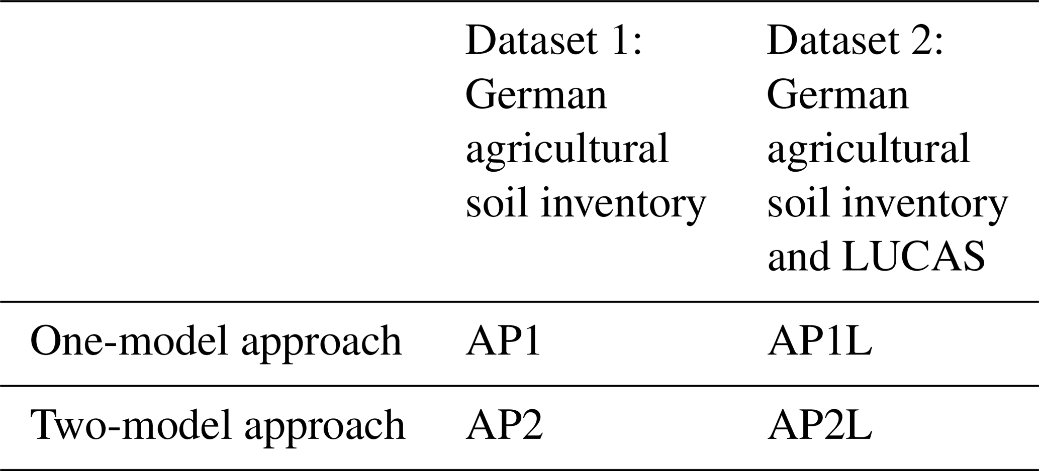
On the one hand, we only used the SOC data from the German agricultural soil inventory and corresponding values from the covariates to train the models (AP1). Due to the high variability in SOC in the agricultural soils of Germany, we then trained two separate models for organic and mineral soils (AP2) to identify whether this could improve model performance. Accordingly, the German agricultural soil inventory was subdivided into mineral and organic soils using a threshold of 87 g kg⁻¹.

The impact of enlarging the training dataset on model performance was then examined for both AP1 and AP2. Thus, 1223 depth-extrapolated samples of the LUCAS data were added to the training sets of AP1. The corresponding modelling approach was named AP1L. Moreover, the above-mentioned threshold (87 g kg⁻¹) was used to subdivide this dataset, and each soil class was included in the training set of the corresponding soil class of AP2. This modelling approach was then named AP2L.

The test sets for the model performance evaluation remained the same for all four approaches to make the results comparable. The results of the AP1 approach served as a baseline on which the model improvement for each algorithm in the other approaches was assessed.

3 Results and discussion

3.1 Comparison of algorithms using data from the German agricultural soil inventory (AP1)

The range of the topsoil SOC content for the German agricultural soil inventory dataset was 4 to 480 g kg⁻¹, with a mean of 27 g kg⁻¹ and a median of 16 g kg⁻¹. Figure 1 shows the spatial distribution of the data. For the first approach (AP1), BRT, RF, and SVR were applied to model SOC using data from the German agricultural soil inventory. The RMSE and MAPE indicated that SVR had a better general performance than the other two algorithms (Fig. 2). In this respect, the RMSE of SVR was 5 % lower than that from RF and 4 % lower than that from BRT. Furthermore, its MAPE was 3 % and 7 % lower than that from RF and BRT respectively. However, despite the difference in overall performance, the spatial distribution of relative residuals indicated that all three algorithms were less accurate in northern Germany compared with the central and southern regions of the country (Fig. 3a). This can be explained by the characteristics of the northern region and its higher SOC variability. The northern part of Germany is lowland that is dominated by a sandy soil texture from Pleistocene sedimentation with geomorphological structures such as ground moraines, terminal moraines, and aprons (Roßkopf et al., 2015). Despite general geomorphological and pedological similarities throughout the region, (1) organic soils under agricultural use are mainly located in the north, and (2) mineral soils with the lowest and highest SOC contents are located in the north-east and north-west respectively. Therefore, the northern region of Germany has the widest SOC range.

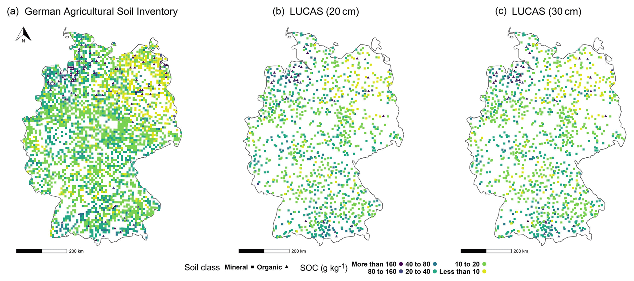
Figure 1 Soil organic carbon content in the topsoil of two soil inventories: (a) the German agricultural soil inventory (0–30 cm) and (b) LUCAS at its original sampling depth (0–20 cm) and (c) after depth extrapolation (0–30 cm).

Figure 2 Performance indicators of the three algorithms: the (a) the RMSE (g kg⁻¹), (b) the MAE (g kg⁻¹), and (c) the MAPE (%) for the one-model approach (without LUCAS data, AP1, and with LUCAS data, AP1L) versus the two-model approach (AP2 and AP2L). The whiskers of the boxplots show 1.5 times the interquartile range. Please note that the y axis is shortened for better visibility and does not display a zero. The abbreviations used in the figure are as follows: BRT – boosted regression trees, RF – random forest, and SVR – support vector regression.

Consequently, the variable importance (Fig. 4a) indicated that the map of organic soils was the most important covariate. The value of the variable importance for this covariate was 65 % in SVR, 72 % in RF, and 84 % in BRT. These values show (1) the crucial role of the map of organic soils for the algorithms in explaining the variability in SOC and (2) the comparatively greater importance of this predictor and the lower variable importance of other predictors in the BRT model compared with the SVR model. Despite the importance of the organic soil map, the scatterplots (Fig. 5a) show that all three algorithms underpredicted the SOC of organic soils and had similar heteroscedasticity patterns in their residuals. Thus, while most residuals from mineral soils followed the 1 : 1 line, they became more scattered in soils with a higher SOC content. The underprediction of SOC in organic soils can be explained by their small sample size, resulting in a dataset with a wide SOC range and a unimodal distribution that leaves these soils in the tail. Consequently, the organic soils were under-represented, and the results were systematically pulled towards mineral soils, irrespective of the choice of algorithm. Different studies have shown that predicting soil properties with mineral and organic soils combined can lead to an underprediction or overprediction of one soil class, depending on the distribution of the dataset (de Brogniez et al., 2015; Guio Blanco et al., 2018; Mulder et al., 2016).

Although the map of organic soils was able to distinguish between the two soil classes (i.e. between mineral and organic soil), it could not separate the mineral soils with a low SOC content in the north-east from those with a high SOC content in the north-west. The spatial distribution of the residuals (Fig. 6a) showed that SVR and BRT generally underpredicted the mineral soils in the north-west part of Germany, whereas RF overpredicted them. Furthermore, unlike RF and SVR, BRT appreciably overpredicted the SOC of north-east Germany's mineral soils, which have the lowest SOC content (<10 g kg⁻¹). This result indicates that the algorithms differed in their performance in mineral soils. This difference was mainly due to the information that they obtained from the land use map. As the second most important covariate for all three algorithms (Fig. 4a), the variable importance value for this covariate was 22 % in SVR, but it was only 11 % in RF and 9 % in BRT. Thus, SVR exploits more information from this covariate than RF and, particularly, BRT. Land use is one of the main drivers of SOC variability on a national scale due to the higher SOC content in grasslands compared with croplands (Poeplau et al., 2020a). Therefore, this covariate was able to differentiate between the soils of the north-east, which are under cropland, and those in the north-west, which are more under grassland. Consequently, the reliance of BRT on the map of organic soils at the expense of land use could explain why this algorithm overpredicted SOC in croplands in the north-east.

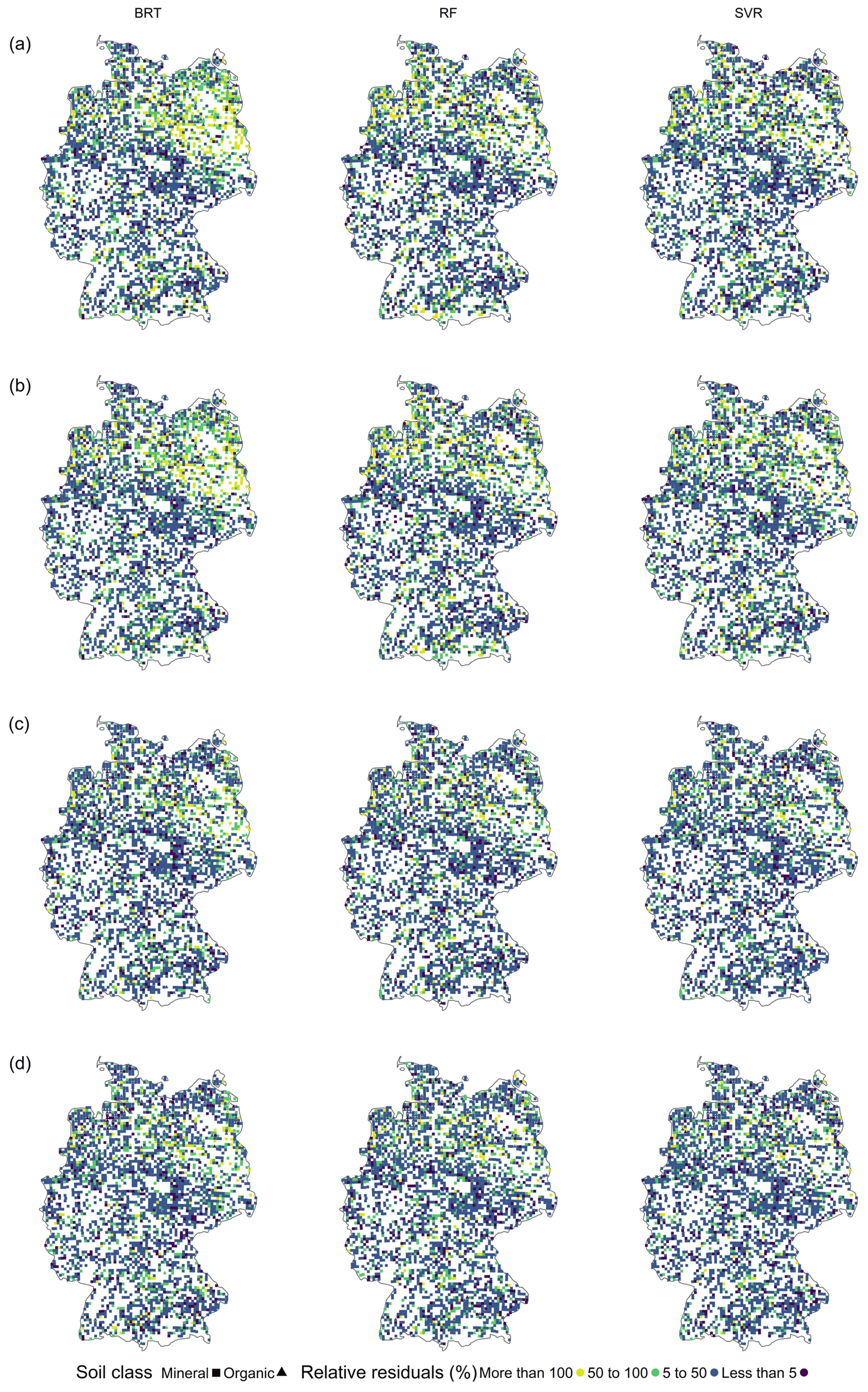
Figure 3 Spatial distribution of relative residuals for (a) the AP1 approach, (b) the AP1L approach, (c) the AP2 approach, and (d) the AP2L approach. The abbreviations used in the figure are as follows: BRT – boosted regression trees, RF – random forest, and SVR – support vector regression.

Figure 4 Variable importance in terms of average relative change (%) in RMSE for (a) AP1, (b) a mineral soil subset of AP2, and (c) an organic soil subset of AP2. The full name for each abbreviation on the y axis is presented in Table S4. The abbreviations used in the headings are as follows: BRT – boosted regression trees, RF – random forest, and SVR – support vector regression.

3.2 Enlarging the dataset with additional soil inventories (AP1L)

A larger soil dataset may provide additional information and, consequently, improve model performance. This possibility was explored in the AP1L approach by adding LUCAS data. The SOC content of LUCAS data at their original depth ranged from 4 to 500 g kg⁻¹, with a mean of 30 g kg⁻¹ and a median of 18 g kg⁻¹. After extrapolating the depth to 30 cm, the new range was from 5 to 512 g kg⁻¹, with a mean of 28 g kg⁻¹ and a median of 17 g kg⁻¹. The spatial distribution of LUCAS data at their original and extrapolated depths is shown in Fig. 1.

A statistical test was performed on the residuals of models built on LUCAS data with the original and extrapolated depths. This was done to identify whether extrapolating the depth of LUCAS data to that of the German agricultural soil inventory would significantly affect model performance after their inclusion in the training set. With the Shapiro–Wilk test rejecting the normality assumption of residuals of all corresponding algorithms at 20 and 30 cm, the non-parametric Kruskal–Wallis test showed no significant difference between the residuals at either depth. Thus, the extrapolation of soil depth had no significant impact on data quality when regionalising the SOC. As a result, any further change in the performance of the algorithms after adding LUCAS data was due to enlargement of the training dataset. The result of the algorithms at both depths can be found in the Supplement (Fig. S3).

After enlarging the training set from 2278 to 3501 sampling points, BRT obtained the lowest RMSE (Fig. 2a1) and MAE among the algorithms (Fig. 2b1). A comparison of the error metrics of corresponding algorithms from the AP1 approach with those from the AP1L approach showed that BRT had the highest error reduction: 7 % in the MAPE and 5 % in the RMSE and MAE. Furthermore, although the error metrics of RF did not improve as much as those of BRT, additional training points were still beneficial for this algorithm. However, SVR did not follow any systematic change using the AP1L approach. Despite a 2 % decrease in the MAPE, the RMSE increased by 3 %, and MAE remained unchanged. To explore the potential explanation for this behaviour by SVR, the residuals of mineral soils were separated from those of organic soils. Additional samples reduced the RMSE in mineral soils for all algorithms by between 9 % and 13 %. However, this error increased by 9 % in the organic subset for SVR, whereas it increased by just 1 % for RF and even decreased by 1 % for BRT. This indicated that enlarging the training set using data with similar characteristics had a greater influence on the systematic error of the under-represented soil class in SVR. This influence is understandable when considering the higher optimised ε in the AP1L approach compared with that of AP1 approach. The higher value of ε means that the hyperplane for the training set is less complex (Cherkassky and Ma, 2004) and, thus, more suitable for predicting most soil samples (i.e. mineral soils). Thus, when this hyperplane was fitted to the same test set as that used in the AP1 approach, the generalisation performance was hindered because it could not capture the variability in samples with higher SOC values (i.e. organic soils).

Further evaluation revealed that, regardless of the change in error metrics, the relative residuals of the three algorithms had a similar spatial pattern to their counterpart from AP1. Thus, they all showed lower accuracy in the northern region of Germany for similar reasons (Fig. 3b). Moreover, the scatterplots had a similar pattern with underpredicted organic soils (Fig. 5b). This confirmed that, when organic soils are modelled with mineral soils, enlarging the training set does not provide enough information for BRT nor RF to capture the high variability in SOC, particularly in the north of Germany.

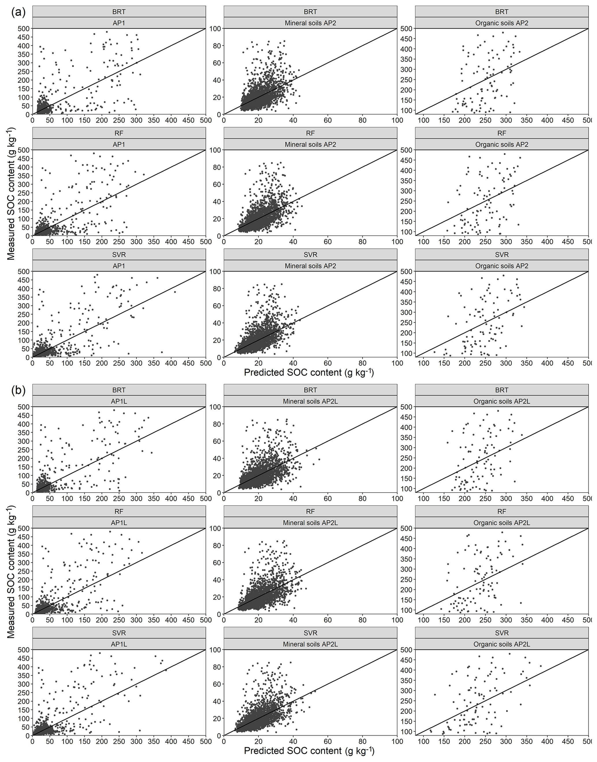
Figure 5 Scatterplot of residuals for (a) the AP1 approach and mineral and organic soils of AP2 and for (b) the AP1L approach and mineral and organic soils of AP2L. The abbreviations used in the figure are as follows: BRT – boosted regression trees, RF – random forest, and SVR – support vector regression.

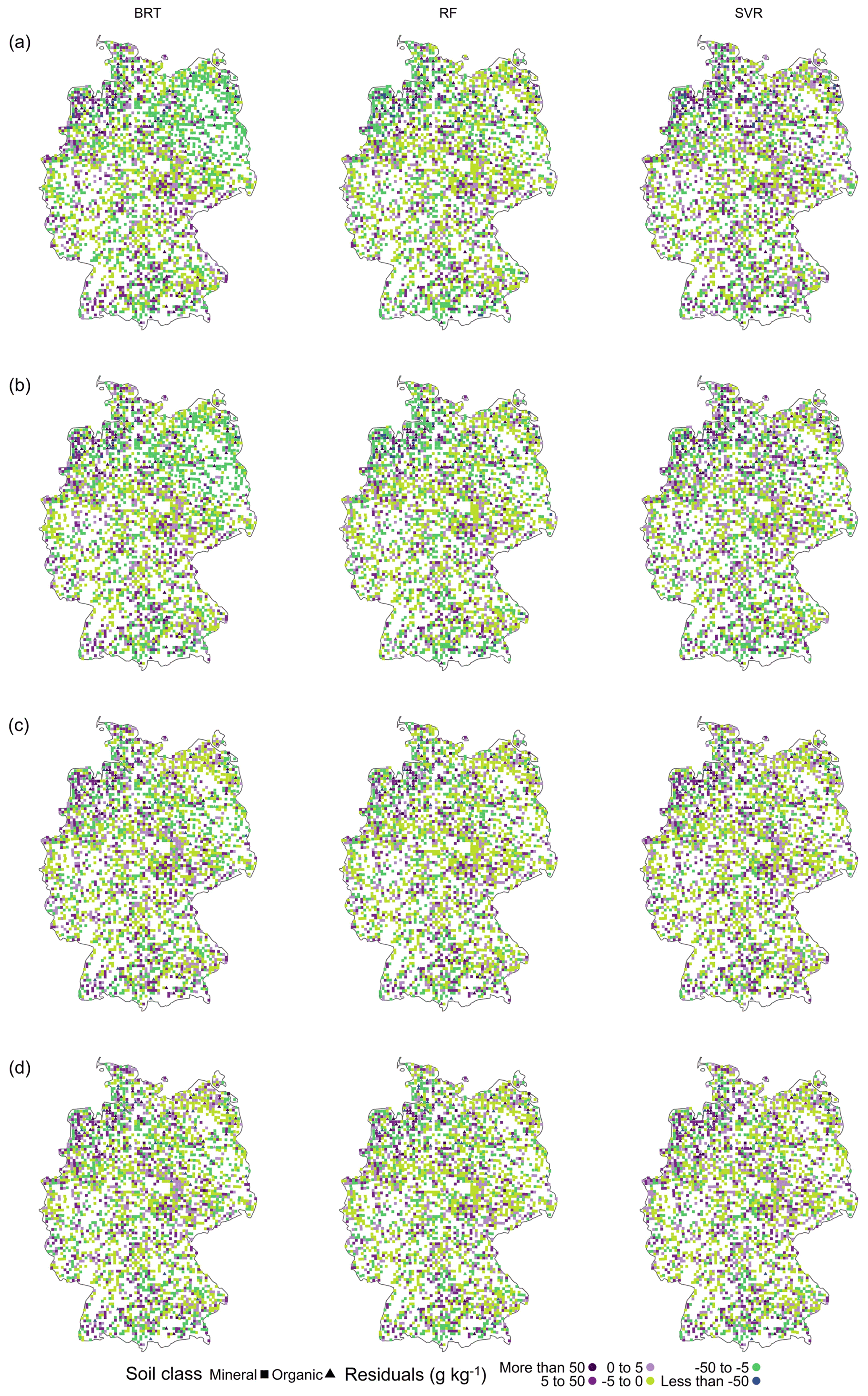
Figure 6 Spatial distribution of residuals for (a) the AP1 approach, (b) the AP1L approach, (c) the AP2 approach, and (d) the AP2L approach. The abbreviations used in the figure are as follows: BRT – boosted regression trees, RF – random forest, and SVR – support vector regression.

3.3 Subdividing soil inventories into mineral and organic subsets (AP2 and AP2L)

As outlined in the sections above, the modelling of the SOC content when mineral and organic soils were combined led to a systematic underprediction of soils with higher SOC values by all three algorithms, irrespective of the number of training samples. Therefore, by implementing the AP2 approach with two models, one for mineral soils and one for organic soils, a noticeable improvement in the performance of all algorithms was observed (Table S3B), with SVR showing the best error metrics (Fig. 2a6, b6, c6). This meant a 34 % lower RMSE, a 30 % lower MAE, and a 32 % lower MAPE than when this algorithm was trained using the AP1 approach with one model for all soils. As the high variability in SOC was initially hard to capture, the subdivision of the dataset provided a range that better represented each soil class. This was particularly beneficial for mineral soils (ranging from 4 to 85 g kg⁻¹) because the number of samples did not decrease drastically (only by 99 samples). Thus, the algorithms could better capture the relationship between SOC and covariates. Consequently, the overall performance improved when the under-represented soil class was modelled separately. This is in line with the study of Rawlins et al. (2009), who recommended the separate modelling of mineral and organic soils.

Nonetheless, following the AP2L approach with additional data, the RMSE and MAPE of the algorithms improved by less than 2 % compared with AP2 (Table S3E). However, the greatest change was observed in the MAE of SVR, which showed a 2 % improvement. Therefore, additional training samples did not greatly influence the performance because the majority of these samples were in mineral soils, while the limiting factor was the high variability in organic soils combined with the low number of samples for this soil class. However, an improvement was noted in relation to all error metrics of SVR in the AP2L approach. This contrasted with when the training set was enlarged without subdividing the data (i.e. AP1L). Therefore, it further confirmed that it is more important for SVR (than for BRT or RF) to model the soil classes separately when the training set is enlarged by datasets with similar characteristics.

Furthermore, the improvement in the algorithms in AP2 and AP2L was particularly noticeable in their relative residuals. By comparing these results with those from AP1 and AP1L, it was evident that the greatest improvement was observed in the northern region, and the spatial distribution of relative residuals was more homogenous throughout the country for all algorithms, although particularly for RF and SVR (Fig. 3c, d). This is understandable because, by subdividing the data, the algorithms can no longer exploit any information from the map of organic soils regarding the spatial variability in SOC in mineral soils. Thus, they obtain information from other covariates for this soil class (Fig. 4b). Although land use and total nitrogen were still among the most important variables for the algorithms in mineral soils, the importance of the predictors representing the SCORPAN C and P factors increased in the absence of an organic soil map. This was to be expected because north-east Germany, for example, has a continental climate (Roßkopf et al., 2015) and young moraine landscapes, whereas the north-west has a more oceanic climate (Roßkopf et al., 2015) with old moraine landscapes.

It is unsurprising that all the algorithms still relied on the map of organic soils to explain SOC in the organic soil class. However, while SVR and RF obtained information from other covariates, the variable importance value of this map alone was 93 % in BRT (Fig. 4c), which makes this algorithm prone to greater errors, as can be seen from its error metrics (Table S2). Similar to mineral soils, the order of covariates was different between the algorithms in organic soils. In other words, in AP1, the three algorithms obtained almost all of the information from the map of organic soils, land use, and total nitrogen in that order of importance. In contrast, after subdividing the data, the algorithms differed from each other with respect to the order of the variable importance of covariates (Fig. 4).

A comparison of the error metrics of each soil class in AP2 with their respective counterparts in AP2L revealed that the additional 1177 samples had a minor influence on the performance (from 0 to a maximum of 2 %) of the algorithms in mineral soils (Table S2). These results indicated that the German agricultural soil inventory offers a good representation of the spatial variability in SOC in mineral soil under agricultural use throughout the country and that the inclusion of more sample points did not provide additional information about SOC variability in this soil class.

However, 46 additional organic soil samples from the LUCAS dataset improved the MAPE and MAE by 12 % and 6 % for SVR, by 10 % and 4 % for RF, and by 7 % and 2 % for BRT respectively, but the RMSE of the three algorithms was improved by less than 2 %. Thus, additional organic samples mainly influenced the average magnitude of the error. This could be explained by organic soils having a wide range of SOC values and by the number of samples being limited. Thus, the addition of LUCAS data to the training set gave the algorithms more information about the spatial variability in SOC in this soil class. Despite this limitation, SVR had the best overall performance among the algorithms in AP2 and AP2L. It should be noted that training samples must span the complexity of the parameter space in order for the model to be able to match the training data effectively and generalise unseen data. Therefore, a small sample size can negatively influence the predictive power of the algorithms. This complexity can be addressed by structural risk minimisation (SRM) (Al-Anazi and Gates, 2012). Implementation of SRM makes SVR capable of performing well on such datasets. Other studies have compared the performance of algorithms on different sample sizes with respect to predicting soil properties and have shown that SVR is one of the best choices, if not the best, when the number of samples is a limiting factor (Al-Anazi and Gates, 2012; Khaledian and Miller, 2020). In contrast, in a study by Zhou et al. (2021), 150 samples with different sets of covariates at different resolutions were used to compare RF, BRT, and SVR to predict the SOC content in Switzerland. Their results showed that the algorithm with the best performance varied depending on the resolution and covariates. However, the best performance throughout all scenarios was obtained by BRT. The discrepancy between their results and the results of the present study may be due to the parameter-tuning method of the algorithms, as they only used grid search or other factors, including the spatial distribution of samples or the chosen set of covariates.

Table 2 Means of the error metrics of the three models for each approach.

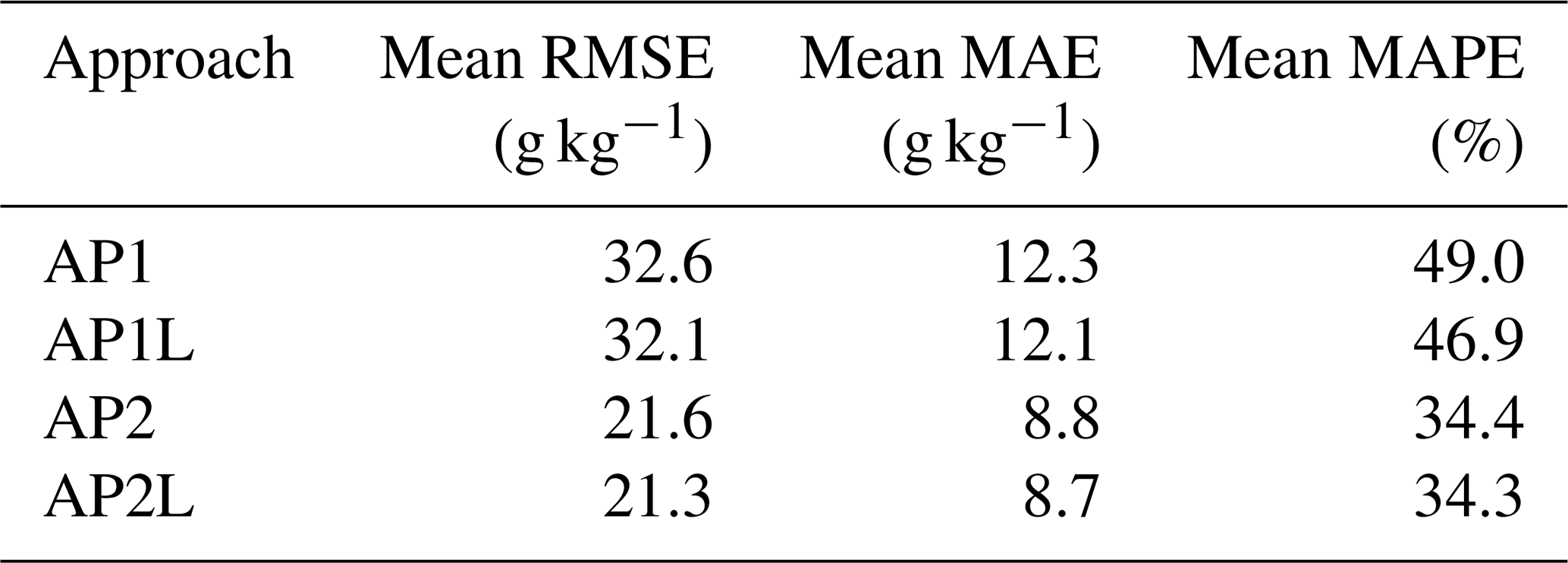
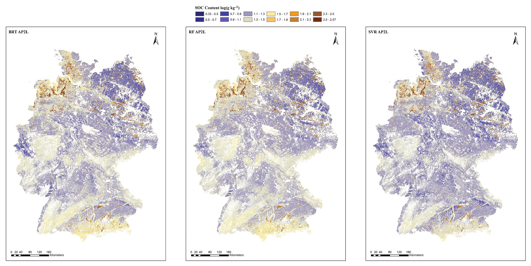
Figure 7 Spatial prediction of the SOC content (g kg⁻¹) of German agricultural soils based on the two-model approach for the three algorithms (BRT AP2L, RF AP2L, and SVR AP2L). The abbreviations used in the figure are as follows: BRT – boosted regression trees, RF – random forest, and SVR – support vector regression. It is important to note that the provided spatial prediction of the SOC content must not be used to identify the organic soils of Germany nor to determine their spatial distribution.

Overall, the change in performance across different sample sizes, different algorithms, and different approaches (Table S3) indicated that the most important aspect of modelling the SOC content of German agricultural topsoil is a two-model approach. Although combining soil inventories for more training samples can possibly improve model performance, the effect was not noticeable compared with when each soil class was predicted by its dedicated model (Table S3B, D). The advantage of two-model approach can also be seen in the average error metrics of the three models (Table 2). While the average RMSE of the models decreases by less than 1 g kg⁻¹ after enlarging the training set, the same error metrics decrease by more than 10 g kg⁻¹ in AP2 and AP2L (Table 2). Therefore, it is also recommended to consider the two-model approach in soil landscape settings similar to Germany or situations where a one-model approach cannot have good predictive performance.

The map of organic soils was used to spatially distinguish each soil class to map the SOC content of the class using its corresponding model. Figure 7 shows the spatial distribution of the SOC content using the AP2L approach for the three algorithms. Although SVR captured a wider range of SOC (2 to 371.5 g kg⁻¹) than BRT (8 to 341.1 g kg⁻¹) and RF (7.7 to 354.6 g kg⁻¹), all three algorithms showed a relatively similar SOC content distribution across the country. In mineral soils, a higher SOC content is mainly found in the north-west and the south, particularly for BRT and RF, whereas the north-east of the country shows a lower SOC content. As explained in the previous sections, one of the main reasons for this distribution is land use, as high-SOC-content regions are mainly under grassland, whereas low-SOC-content regions are under cropland. As shown in Fig. 7, organic soils are mainly distributed in the north. Most bog peat soils are located in the north-west, whereas fen peat soils can be found both in the north-west and in the north-east (Roßkopf et al., 2015). Smaller areas of all types of organic soils can be found in the moraine landscapes and the foothills of Alps in the south. It is important to note that the provided spatial prediction of the SOC content must not be used to identify the organic soils of Germany nor to determine their spatial distribution. One reason for this is the low sample size of organic soils and the systematic underestimation of their SOC content, which leads to an underestimation of their spatial extent. Furthermore, the present analysis is limited to the topsoil, but organic soils might have been mixed with mineral soil (i.e. due to deep ploughing) or feature a mineral soil cover. Thus, organic soils might be present despite the presence of a mineral topsoil. Finally, some of the data used for the derivation of the map of organic soils are subject to improvement; thus, modifications in spatial distribution are expected. Therefore, this study cannot (nor does it intend to) delineate or classify organic soils.

4 Conclusions

The three algorithms most commonly used in DSM were applied to predict the SOC content of German agricultural soils using different approaches. Suitable tuning strategies for each algorithm ensured optimum parameter tuning and made their performance truly comparable. Machine learning was shown to be powerful at modelling SOC on a national scale. However, the study showed that separate modelling of mineral and organic soils was a better approach for modelling SOC compared with just one model. Thus, this approach takes priority over the choice of algorithm and number of training samples. Further testing of this approach is recommended in countries and regions that cover both of these soil classes. Nonetheless, SVR had a better performance than RF and BRT, except when the number of samples in training was increased by additional dataset. This was disadvantageous for SVR and advantageous for BRT unless mineral and organic soils were modelled separately. In general, increasing the number of training samples led to a limited improvement in performance. Therefore, when adopting this approach, consideration should be given to the algorithm and the characteristics of the data. Furthermore, the better performance of SVR compared with that of RF and BRT was particularly highlighted when predicting SOC in organic soils. The good performance of SVR suggests that this algorithm should be taken into greater account in DSM.