the Creative Commons Attribution 4.0 License.
the Creative Commons Attribution 4.0 License.
 | 24 Aug 2022
On the benefits of clustering approaches in digital soil mapping: an application example concerning soil texture regionalization
Mareike Ließ
High-resolution soil maps are urgently needed by land managers and researchers for a variety of applications. Digital soil mapping (DSM) allows us to regionalize soil properties by relating them to environmental covariates with the help of an empirical model. In this study, a legacy soil dataset was used to train a machine learning algorithm in order to predict the particle size distribution within the catchment of the Bode River in Saxony-Anhalt (Germany). The random forest ensemble learning method was used to predict soil texture based on environmental covariates originating from a digital elevation model, land cover data and geologic maps. We studied the usefulness of clustering applications in addressing various aspects of the DSM procedure. To improve areal representativity of the legacy soil data in terms of spatial variability, the environmental covariates were used to cluster the landscape of the study area into spatial units for stratified random sampling. Different sampling strategies were used to create balanced training data and were evaluated on their ability to improve model performance. Clustering applications were also involved in feature selection and stratified cross-validation. Under the best-performing sampling strategy, the resulting models achieved an R2 of 0.29 to 0.50 in topsoils and 0.16–0.32 in deeper soil layers. Overall, clustering applications appear to be a versatile tool to be employed at various steps of the DSM procedure. Beyond their successful application, further application fields in DSM were identified. One of them is to find adequate means to include expert knowledge.
- Article
(11041 KB) - Full-text XML
- BibTeX
- EndNote


In order to sustain soil resources, land managers and researchers are in need of information on the continuous landscape-scale distribution of soil properties. One of the important soil properties which governs most physical, chemical, and biological soil processes is soil texture. Soil texture maps can be used for the assessment of erosion risk, water deficit, or pesticide and nutrient storage and percolation (Blume et al., 2016).
Conventional soil maps are usually created by a qualitative analysis of the landscape based on a conceptual model which subdivides the area into spatially assigned units with all soil properties set to uniform values within the units. The categories of these units do not necessarily represent soil systematic units and do not allow for the representation of small-scale, continuous variability. Overall, these soil maps were never meant to be used as input to landscape-scale process models that strive to simulate gas, matter and water flows. From this demand and an advance in information technology, the domain of digital soil mapping (DSM) has quickly advanced (Grunwald et al., 2011).
DSM strives to capture and quantify the influence of the soil-forming factors, which are represented by continuous gridded geoinformation from remote sensing and other sources (Scull et al., 2003). Laboratory and field observations are coupled with spatial environmental covariates covering the study area and are used to build an empirical model to predict the surveyed target variable based on the quantitative relationship between soil properties and environmental covariates (McBratney et al., 2003; Grunwald, 2009; Minasny and McBratney, 2016). The key technological advantages that allowed DSM are the increase in computational power which facilitates model development and the widespread availability of satellite systems (Rossiter, 2018). The latter are used for accurate georeferencing and as platforms for a variety of sensors which provide spatially continuous measurements which can be used as environmental covariates.
The algorithms used for DSM applications are of different degrees of complexity, ranging from linear regression (Gobin et al., 2001; Park and Vlek, 2002; de Carvalho Junior et al., 2014) to artificial neural networks (Park and Vlek, 2002; Zhao et al., 2009). Most of these studies used continuous covariates based on a digital elevation model (DEM) as predictors, but certain applications also included categorical covariates, such as information based on geologic maps (Adhikari et al., 2013; Vaysse and Lagacherie, 2017). The machine learning algorithm most frequently used in DSM approaches is the random forest (RF) ensemble learning method (Padarian et al., 2019). A key characteristic of RF is its adaptive nature which allows it to explore complex, nonlinear, and high-dimensional relationships without a prior understanding of the problem to be solved (Evans et al., 2011). Compared to decision tree methods, RF is less prone to overfitting and is less sensitive to irrelevant predictors and outliers (Heung et al., 2014). Nevertheless, many RF and other modelling applications use feature selection preceding the model-building procedure to detect and exclude predictors with little information content with regards to the response variable. Feature selection can be achieved though filter methods, which investigate the predictor–response relationship of each predictor individually without considering the model algorithm, or alternatively by using wrapper methods that evaluate the performance of the model using a variety of predictor subsets.
The essential foundation of creating soil maps is the availability of a soil dataset of sufficient size and adequate distribution, but the soil surveys providing these data are associated with high cost and labour (Grunwald et al., 2011). To forego this effort, DSM uses legacy soil data whenever available. However, sampling in traditional soil surveys usually did not follow statistical sampling theory, which can lead to a bias in the data and the models derived from it (Carré et al., 2007; Ließ, 2020). Because soil-forming factors operate on different scales, it is important that the spatial distribution of the data is suitable for capturing the large- and small-scale variation of soil. In order to construct a model that can effectively predict throughout the landscape, it is important to have a statistically representative sample of training and validation data that allows for the generalization from the data to the spatial landscape context (Ließ, 2020). The most common approaches in dealing with this issue involve (a) creating a more balanced training set by sampling from the entirety of observations and (b) cost-sensitive learning frameworks, in which the learning algorithm penalizes the prediction error of underrepresented samples (He and Garcia, 2008). Many DSM applications tackle the problem of data imbalance with the subsampling approach (Moran and Bui, 2002; Subburayalu and Slater, 2013; Heung et al., 2016; Sharififar et al., 2019). This can be achieved by clustering the study area into homogeneous subareas with regards to the covariates and drawing a certain number of samples from each of these clusters.
Another hurdle of modelling applications lies in training and tuning. Model building and performance evaluation can be sensitive to the data splitting into training and testing sets. Although resampling techniques like cross-validation (CV) reduce the influence of data splitting, the model outcome can still be compromised by an uneven distribution of sample characteristics between training and testing datasets.
Many of these challenges in the DSM procedure are related to identifying structures and similarities in the data. Therefore, here we want to investigate the usefulness of data-clustering applications in tackling some of the above-mentioned challenges in DSM. Specifically, we want to examine the benefits of using clustering applications for feature selection, for landscape stratification to conduct data subsampling, and for stratified cross-validation to build robust models. This will be done on the basis of training an RF model to predict soil texture within the catchment of the Bode River in Saxony-Anhalt, Germany. The model is trained and validated using a soil legacy dataset containing soil survey data. Environmental covariates related to soil-forming factors are obtained and used as predictors.
2.1 Study area and data
2.1.1 Study area
The study area of approximately 3300 km3 is part of the TERENO network for environmental observations (Zacharias et al., 2011) and covers the water catchment of the Bode River in central Germany (Fig. 1). It corresponds to three federal German states: Saxony-Anhalt, Lower Saxony, and Thuringia. The elevation ranges between 1 and 1141 m a.s.l. with the Harz Mountains in the south-west, the north-eastern Harz foreland, and the Magdeburg Börde of the North German Plain covering the rest of the area. The climate is subarctic to humid continental (Peel et al., 2007), with the mean annual precipitation ranging from 433 to 1771 mm (Deutscher Wetterdienst, 2020). The geologic material in the area consists mostly of Triassic limestone and Carboniferous shale and granite (BGR, 2007). Dominating soils according to the German soil classification (Finnern and Kühn, 1994) are Braunerde, Parabraunerde, Gley, and Pararendzina (BGR, 2012).

Figure 1Study area (a) location in Germany, (b) location of the survey sites, (c) and cross-sectional elevation profile (black line on the map).
2.1.2 Soil legacy data
The soil samples used for model training and validation are from a legacy dataset provided by the regional geological survey of the German federal state of Saxony-Anhalt – Landesamt für Geologie und Bergwesen (LAGB, 2018). The data were recorded by various soil surveyors between 1963 and 2006 and consist of soil profile data from 574 sites. For every site, a soil diagnostic survey was conducted. Soil horizon boundaries were recorded according to either the TGL (TGL, 1985) or KA4 (Finnern and Kühn, 1994) soil systematic system. For every soil horizon, the particle size distribution was measured in the laboratory using DIN ISO 11277:2002-08. The fractions of three particle sizes were measured according to the German soil separates (sand [2 to 0.063 mm], silt [0.063 to 0.002 mm], and clay [< 0.002 mm]). Sand, silt, and clay contents were extracted from the horizon data at two discrete soil depths (10 and 70 cm) and used as the response variables of the models. The two depths were chosen to investigate whether different soil-forming factors dominated soil-landscape development in the topsoil and subsoil, respectively. Because the maximum depth of the surveyed soil profiles is not uniform, a depth of 70 cm was chosen as a trade-off between maximum soil depth (closeness to parent material) while not compromising the sample size. One sample is located in a Quaternary sand dune of less than 2 km2 (BGR, 2007) near the town of Blankenburg and has a sand content of 96 %. The sample was removed because one sample alone would not be sufficient for model training and validation. The soil texture of the soil legacy dataset used for model training and evaluation is shown in Fig. 2a and b. A cluster analysis targeting three equally sized subgroups was applied to differentiate clayey samples from silty and sandy samples; please refer to the “Cluster analysis” section for details. Figure 2c and d show the spatial distribution of these three clusters within the study area.
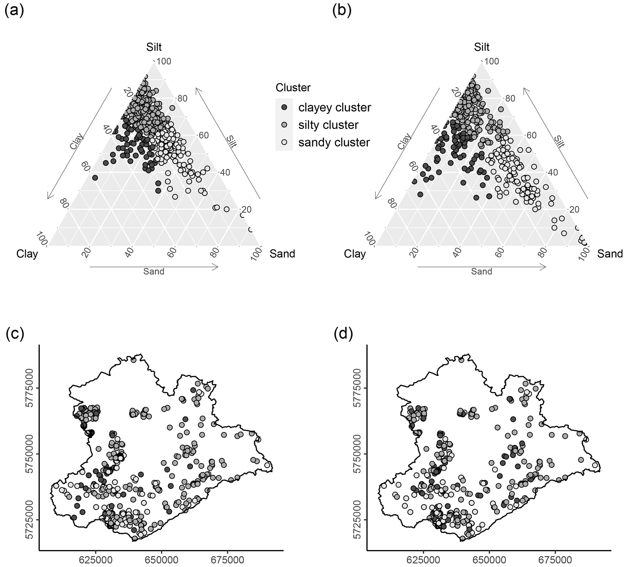
Figure 2Soil legacy dataset used for model development. Particle size distribution and cluster affiliation of the soil data at (a) 10 and (b) 70 cm depth, respectively. Panels (c) and (d) show the spatial distribution of the three clusters at 10 and 70 cm depth (geographic coordinate system: UTM zone 32∘ N).
2.1.3 Model predictors
Spatially continuous geodata of the study area corresponding to the soil-forming factors parent material, topography, and land cover were gathered. They comprise geologic maps of 1 : 200 000 (GUEK 200) and 1 : 1 000 000 (GUEK 1000) map scale (BGR, 2007, 2006), a DEM of 10 m resolution (BKG, 2012), and CORINE Land Cover data from 1990, 2000, and 2012 (Büttner et al., 2004). The local river network was generated from the OpenStreetMap dataset by querying rivers and streams with the Overpass API service (OpenStreetMap contributors, 2018). Some of the geodata were used without further modification, like the land cover data and the elevation from the DEM. Additionally, further predictors were derived from these data and have been resampled to the 10 m resolution of the DEM.
In the digital vector information underlying the geologic maps, a variety of attributes is contained, including age, material, and origin. The “petrography” layer was used from both geologic maps, and the “genesis” layer was used from the 1 : 200 000 map. As the information contained in the petrography layer is descriptive, it was categorized into binary information on the occurrence of particle size classes in addition to its inclusion as an unmodified layer. Three new predictors (Sandbin, Siltbin, and Claybin) were created for every landscape unit based on the occurrence of the words sand or sandstone, silt or siltstone, and clay or claystone, respectively.
Several topographic predictors were derived from the DEM, since relief is often considered the main driver of soil formation (McBratney et al., 2003; Scull et al., 2003; Behrens et al., 2010). Topographic predictors were calculated with the SAGA GIS software Version 6.4.0 (Conrad et al., 2015). The used topographic predictors were selected according to their appearance in similar digital soil mapping applications (Bulmer et al., 2016; Vaysse and Lagacherie, 2017; Blanco et al., 2018; Kalambukattu et al., 2018; Zhou et al., 2019; Table 1). Sink removal by Wang and Liu (2006) was applied prior to the calculation of the hydrological terrain parameters (minimal slope = 0.01). For the calculation of the vertical distance to the channel network, the layer of waterways acquired from OpenStreetMap was used. Indices for terrain convexity and terrain surface texture were calculated by using a flat area threshold of 0.08 in order to minimize the impact of inaccuracies and insignificantly small depressions and mounds (Conrad et al., 2015).
Since soil-forming factors can take effect on different spatial scales, it is advised to take multiscale approaches into account (Behrens et al., 2010). Accordingly, convergence index (Köthe and Lehmeier, 1996), terrain ruggedness index (Riley, 1999), convexity, and terrain surface texture were calculated with a search radius of 10, 50, 100, and 200 m in order to express local to regional landscape attributes. The annulus-based topographic position index (Guisan et al., 1999) was calculated on two scales, one ranging from 0 to 100 m and one from 100 to 200 m.
Zevenbergen and Thorne (1987)Köthe and Lehmeier (1996)Friedrich (1996)Böhner and Selige (2006)Böhner and Selige (2006)Böhner and Selige (2006)Böhner and Selige (2006)Böhner and Selige (2006)Riley (1999)Conrad et al. (2015)Conrad et al. (2015)Guisan et al. (1999)Yokoyama et al. (2002)Yokoyama et al. (2002)Böhner and Antonić (2009)Böhner and Antonić (2009)Bock et al. (2007)Böhner and Selige (2006)Moore et al. (1991)Beven and Kirkby (1979)Marchi and Dalla Fontana (2005)Conrad et al. (2015)Table 1Topographic predictors derived from the digital elevation model. Indices that have been calculated with varying window sizes are denoted by multiscale.

2.2 Modelling procedure
2.2.1 Random forest
RF models are based on regression trees (RTs), which use selected values of predictor variables to repeatedly split the data in a way that maximizes the homogeneity of the subsets regarding the response variable (Kuhn and Johnson, 2013). Instead of building a single tree as is the case in RTs, RF uses the bagging ensemble method which constructs several trees based on bootstrapped samples of the data. The resulting averaged prediction has a lower variance and thus increased model stability compared to RTs. Although randomness is added to the procedure through resampling of the data, the underlying predictor–response relationship is not altered by bagging. As a consequence, many of the trees share similar structures. This correlation between trees can lead to a decrease in the predictive performance of the ensemble (Breiman, 2001). To introduce diversity to the ensemble and decorrelate the trees, RF is extended by a random feature selection. Instead of using the entire set of predictors to build a tree, a random subset of the predictors is used for each tree. This reduction of predictors leads to a trade-off between the strength of individual trees (high number of predictors) and more diversity between trees (low number of predictors). The respective tuning parameter, which controls this trade-off, is “mtry”, the size of the predictor subset. Further parameters include “ntree”, the number of trees, and “nodesize”, the minimum number of samples to be kept in a terminal node of the trees (Were et al., 2015).
For the interpretation of the RF models, the model function calculates a variable importance measure. This is done by building models which use permutations of a predictor variable. The accuracy of the permuted model is then compared to a model built from the original data. The returned value indicates the decrease in prediction accuracy after permutation.
2.2.2 Cluster analysis
A cluster analysis (CA) was conducted for several purposes.
-
CA-1: feature selection and process understanding
-
CA-2: landscape stratification into subareas for subsampling
-
CA-3: data stratification in the CV approach
In CA-1, k-means clustering was used to split the soil texture data of both depth levels into three clusters to distinguish between sandy, silty, and clayey soils (Fig. 2). The distribution of every predictor value among the three clusters is analysed to (a) determine whether the predictor has any influence on soil texture (feature selection in Sect. 2.2.3) and (b) gain process understanding by analysing the relationship between predictors and soil texture. The clustering was performed with the k-means function using 40 initializations for each of the 30 iterations on the centre-scaled sand, silt, and clay contents. The resulting clusters' predictor ranges at the assigned soil survey sites were retrieved.
CA-2 was applied for landscape stratification into homogeneous subareas on behalf of the gridded continuous multivariate predictor data. These data, however, have certain traits which provide a challenge to cluster analysis. These traits are the high dimensionality of the data, correlation between predictor variables, and its consistency of numerical as well as categorical predictors. These issues were tackled by applying a factor analysis of mixed data (FAMD) from the FactoMineR package (Lê et al., 2008) to the dataset. Because of the high resource demand of conducting an FAMD on the whole dataset (33 million grid cells), the function was applied to a random data subset of 100 000 samples first, and then the resulting FAMD model was applied to the whole dataset. In order to allow for the application of the function for FAMD transformation trained on the data subset to the complete dataset, the minimum and maximum values of all numerical predictors and all classes of the categorical predictors were additionally included. The FAMD returns n factors, with the percentage of explained variance decreasing with every factor. A reliable method to determine the number of dimensions to retain from the FAMD is the “elbow” approach (Linting et al., 2007). The contribution of each retained dimension to the percentage of explained variance decreases strongly with the first dimensions until it reaches a nearly constant value. The “elbow” approach suggests using all dimensions before the stagnation of the explained variance. The resulting FAMD-transformed data were clustered using k-means in CA-2.
The number of clusters was determined by the use of cluster validation indices calculated with the NbClust function from the NbClust package (Charrad et al., 2014). The function calculates 27 clustering indices for each clustering solution in a given range of number of clusters. All of the clustering indices cast their vote for their favoured number of clusters. Because of the high computational cost, the function was repeatedly applied (2000 times) to random data subsets of size 2000 of the data resulting from the FAMD. Preliminary test runs have shown that a sample of size 2000 produced stable clustering results. A number of 2 to 17 clusters was tested.
CA-3 was conducted in order to perform a stratified CV. Stratification was conducted on behalf of the response variable. In a first step, the legacy dataset including sand, silt, and clay content was clustered into five equally sized subgroups. From each of the subgroups, the profiles were then in a second step equally assigned to the k folds in order to obtain a similar data distribution in each of the k folds. The clustering was achieved by using a same-size k-means algorithm (Schubert and Zimek, 2019) to divide the profiles of both depth levels into five clusters based on the soil texture.
2.2.3 Feature selection
The RF algorithm is relatively robust against uninformative predictors by only selecting the strongest predictors as a splitting criterion (Hamza and Larocque, 2005; Kuhn and Johnson, 2013), and even though the reduction of the predictor set may not necessarily improve model performance, it can still benefit model interpretability and reduce computational time (Chandrashekar and Sahin, 2014). However, the feature selection based on CA-1 was not only conducted to remove uninformative predictors, but also to study the predictor–response relation.
The clustered profiles were paired with the corresponding predictor values. The Kruskal–Wallis test was used to compare the distributions of predictor values between the three clusters. The resulting p values were adjusted for multiple comparison by controlling the false discovery rate (Benjamini and Yekutieli, 2001). All predictors with significant differences in means between the three clusters (α=0.05) were used as predictors for the RF models of the respective depth levels. To gain further insight into the predictor–response relationship, Dunn's test was performed on these predictors as a post hoc analysis. This allows us to determine which clusters show significant differences concerning the particular predictors.
Preliminary results have shown that categorical predictors and the usage of the Cartesian coordinate space can lead to artefacts in the maps of predicted soil texture. Two more models were built in addition to the model using the full predictor set (full) in order to tackle this problem. One model leaves out the petrography and genesis layers as predictors (no geo), and the other leaves out petrography, genesis, longitude, and latitude (no geo + coords).
2.2.4 Strategies for unbalanced data
Statistical sampling from the soil dataset was used in order to create training and validation data better balanced in regard to landscape characteristics corresponding to the interaction of the soil-forming factors. Please compare Ließ (2015, 2020) concerning a detailed discussion of this aspect. This was done by applying four subsampling approaches to the model training data based on the landscape clusters obtained from CA-2. Performance of the models trained on the thereby adapted data was compared to that of models built with the legacy dataset in its original distribution. Subsampling was conducted to match the spatial coverage of the landscape clusters (area-weighted method: AW) or in order to provide a sample that represents each landscape cluster with the same amount of data (equal number approach: EN) (similar to Heung et al., 2016). The subsampled dataset is obtained either by oversampling or undersampling (He and Garcia, 2008). Oversampling obtains the dataset by including all samples from all clusters and then replicating certain randomly selected samples until the desired sample size for each cluster is reached. Undersampling includes all samples from the minority cluster and then randomly draws samples from all other clusters until the desired sample size is obtained. The four applied sampling approaches are displayed in Fig. 3.
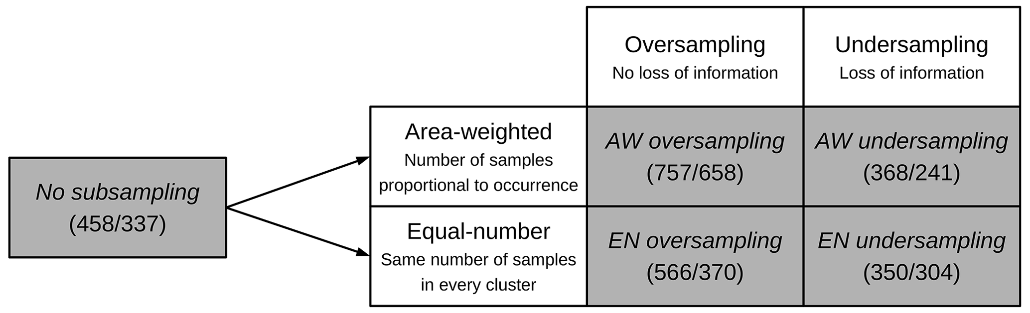
Figure 3Applied sampling approaches. Parentheses show the number of samples in the training set (10 and 70 cm depth, respectively). Abbreviations of the sampling methods as used in the results are shown in italic.
2.2.5 Model training, tuning, and evaluation
Model tuning and evaluation for the RF models was conducted by a nested approach of repeated stratified 5-fold CV (5 repetitions). The detailed procedure is shown in Fig. 4a. As a performance measure, the root-mean-square error (RMSE) was derived. In order to make the model performance values comparable for all models, the respective test set was kept the same, while data subsampling was only applied to the respective training sets (Fig. 4b). Furthermore, response data were centred and scaled (SD = 1) to allow for the comparability of model performance between models targeting sand, silt, and clay content. The k folds of the nested approach were derived by stratified sampling regarding the response data. In order to stratify the dataset regarding all three response variables at once, response strata were formed by applying CA-3. Tuning takes place in the inner CV, where the model is evaluated for mtry parameter values within the range of 5 to 25, while ntree was set to 1000 and nodesize to 5. Overall, the model-building procedure was applied six times in order to create individual RF models for each of the three particle sizes for the two soil depths.
For the data analysis and modelling, R version 3.5.1 was used (R Core Team, 2018). All computation was performed on a machine running Windows Server 2016 Standard with four Intel® Xeon® Processor E7-8867 v4 and 6.00 TB of memory.
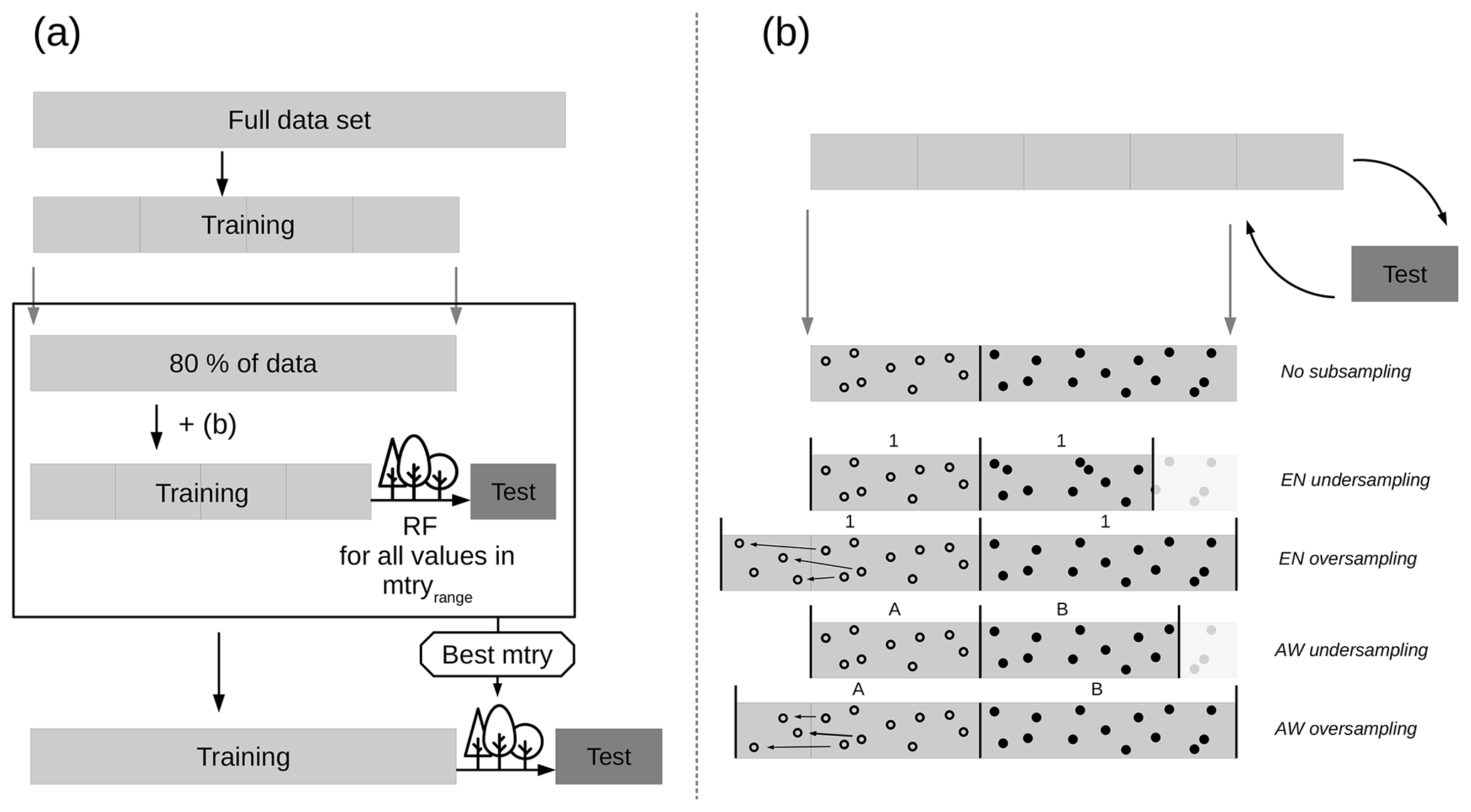
Figure 4Nested k-fold CV approach for model tuning and evaluation. General approach without data subsampling (a). Incorporation of the subsampling strategies in the CV approach (b).
3.1 Exploratory data analysis
3.1.1 Feature selection
The soil profiles used for model building were split into three groups based on their soil texture with CA-1. A clayey cluster was, thereby, distinguished from a silty cluster and a sandy cluster. Primarily, this was done in order to understand which predictors are best at separating these three groups and therefore are expected to have a high explanatory power in the models to predict spatial soil texture distribution within the investigation area. The soil texture of the profiles at 10 and 70 cm depth and their cluster affiliation is shown in Fig. 2a and b. The spatial distribution of the clusters is shown in Fig. 2c and d. The distribution of cluster affiliation within the study area shows that most of the profiles in the lowlands belong to the silty cluster. This is typical for the soils of this area, which are influenced by loess deposits.
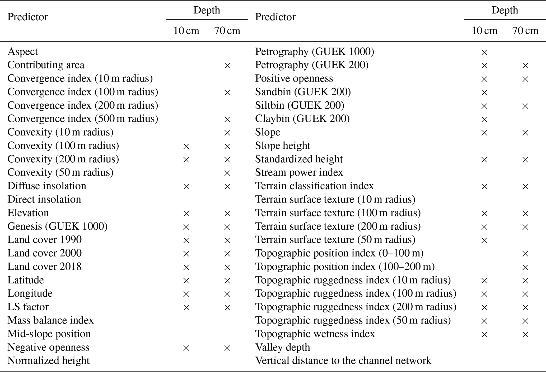
The predictor data at each sampling site were assigned to the soil profile data. The data distribution of the predictors between the three soil texture clusters was then compared by applying a Kruskal–Wallis test. Out of 39 numeric predictors, 27 predictors showed a significant difference of the mean at either 10 or 70 cm depth (Table 2). The predictors displaying significant differences between any two of the soil texture clusters were included in the random forest models. The trends in differences between the clusters are predominantly in agreement across the two depth levels (Fig. 5). For many of the predictor values with significant differences in the means, it was the silty cluster that was the most distinguishable from the other two clusters. From the 54 statistical tests (27 significant predictors for two soil depths), 51 showed differences between the sandy and silty clusters and 28 showed differences between the clayey and silty clusters, while only 19 tests showed differences between the sandy and clayey clusters.

Figure 5Data distribution of selected predictors per soil texture cluster and soil depth. Letters above boxplots denote significance groups within one depth level. The y axes are cropped to highlight the interquartile range.
Since the clustering application used here for feature selection is a filter method, it is unable to take interactions between different predictors into account. This could compromise the efficacy of the feature selection if there are predictor–response relationships which are only revealed in combination with other predictors. The advantage of the clustering method is to create meaningful categories in the data and investigate their relationship with the predictor values, which cannot be provided by a wrapper method.
Table 2Predictors included in the random forest model for 10 and 70 cm depth, denoted by “×”.
3.1.2 Landscape stratification for subsampling approaches
CA-2 was conducted in order to subsample from the legacy soil dataset and create a balanced model training set. The FAMD data transformation showed an increased drop of explained variance with the sixth factor, resulting in the first five factors being used as input for CA-2. The NbClust application resulted in 29 % of the votes being appointed to finding two clusters in the data, while the second-largest vote was 13 % in favour of three clusters. Hence, the environmental data of the study area were divided into two clusters using k-means. The resulting clusters broadly divided the study area into the mountainous region and the lowlands (compare Fig. 1). This way of stratifying the landscape is an apparent choice, since the relatively low number of training samples suggests taking a small number of clusters to have sufficient samples per cluster. Further, the heuristic approach of dividing the landscape, which is often superior to automated classification (MacMillan et al., 2004), also suggests the separation between the highlands and lowlands due to the relatively sharp divide.
3.2 Model development
3.2.1 Model performance
The predictive performance of the RF models was investigated under different subsampling approaches, a range of mtry tuning parameter values, and three predictor sets. Since the RMSE values for model evaluation were calculated for the modeled response variables scaled to an SD of 1 to provide a comparable metric, the RMSE values can be interpreted as zero being perfect predictability and values over one meaning a worse performance than using the observed mean as the predicted value. The RMSE values of all subsampling approaches for the full predictor set are shown in Fig. 6. The median RMSE is between 0.67 and 0.94, with the silt and sand models clearly outperforming the clay models. For all particle size classes, model performance is better for 10 cm compared to 70 cm depth, with an average difference in the RMSE of 0.08 for clay and silt and 0.12 for sand. This decrease in performance may be due to a decrease in sample size with soil depth. Studies where sample size have been consistent along profile depth have shown that the predictive performance does not necessarily decrease with soil depth (Adhikari et al., 2013; Vaysse and Lagacherie, 2015).
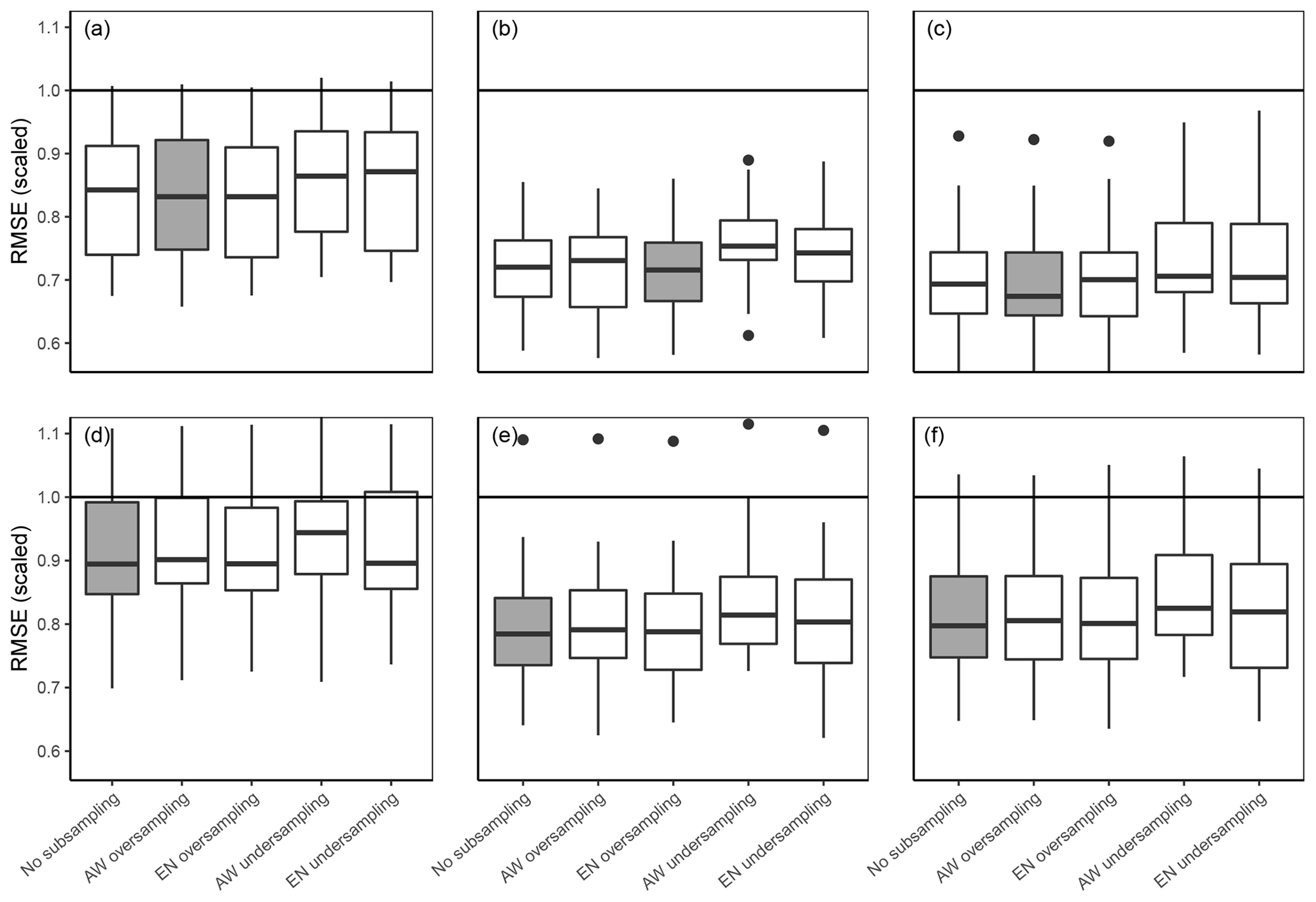
Figure 6Model performance as boxplots of RMSEs of the five repetitions for three particle size contents for (a, d) clay, (b, e) silt, and (c, f) sand and five subsampling methods. The models (a), (b) and (c) are for 10 cm depth, while (d), (e), and (f) are 70 cm depth. The subsampling method with the lowest median RMSE is highlighted. The black horizontal lines stand for an RMSE of one, which equals the RMSE of predicting the observed mean.
There is no consistently better-performing subsampling method. However, both undersampling approaches seem to have higher median RMSE values than the two oversampling methods. It seems likely that the decline in model performance was due to the reduction of the sample size. Using the RMSEs of the whole study area as the selection criteria for the subsampling approach also has its limitations because it does not provide information on the spatial distribution of the prediction accuracy. Adding more weight to samples of a certain cluster can lead to increased accuracy in the respective area, while this gain is not necessarily covered by the validation data. The role of subsampling in the distribution of prediction accuracy is exemplarily displayed in Fig. 7. Although there are strong differences in the overall accuracy between clusters, neither of them profits explicitly from a certain subsampling method. The right choice of the subsampling method most likely depends on the underlying data, since other DSM studies have not revealed a distinctly better-performing method. While the EN approach increased model accuracy for the minority class in Heung et al. (2014), Schmidt et al. (2008) found the contrary effect in their study and Moran and Bui (2002) found AW to be the best-performing model. Sharififar et al. (2019) used a combination of oversampling and undersampling to create a balanced dataset which significantly improved model performance, while oversampling and undersampling decreased model performance in Taghizadeh-Mehrjardi et al. (2019).
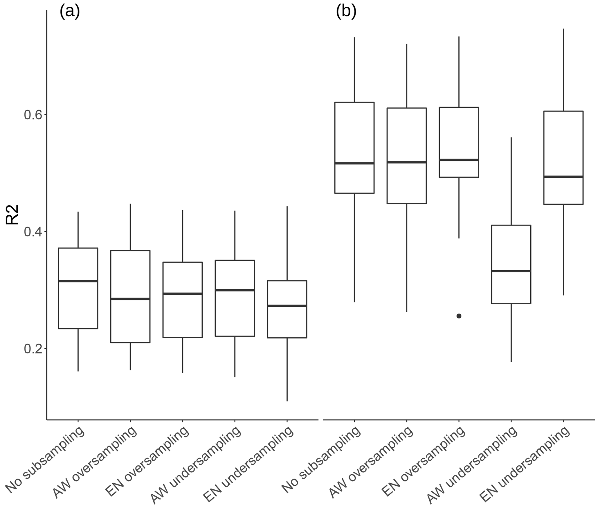
Figure 7Landscape cluster-specific model performance of the silt model at 10 cm depth with panel (a) showing the R2 of the samples from the lowlands cluster and panel (b) the samples from the mountainous cluster.
In order to prevent the occurrence of artefacts, predictors have been retained from model building. This led to a decrease in model performance across all particle sizes and depth layers (Fig. 8). The no geo + coords models showed an average increase in scaled RMSE of 3 %, 7 % and 12 % for sand silt and clay at 10 cm depth when compared to the full model.
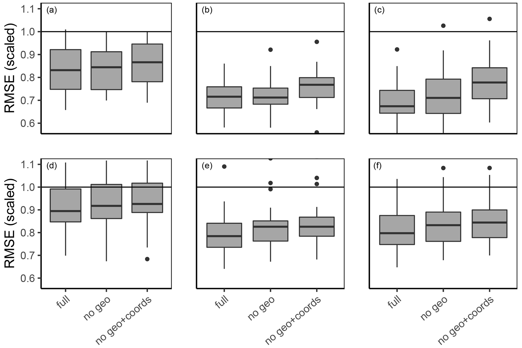
Figure 8Model performance as RMSE for three particle size contents for (a, d) clay, (b, e) silt, and (c, f) sand. The models (a), (b), and (c) are for 10 cm depth, while (d), (e), and (f) are for 70 cm depth. Models were built using either all predictors (full), leaving out the geologic predictors (no geo) or leaving out geology, latitude, and longitude (no geo + coords). The black horizontal lines stand for an RMSE of one, which equals the RMSE of predicting the observed mean.
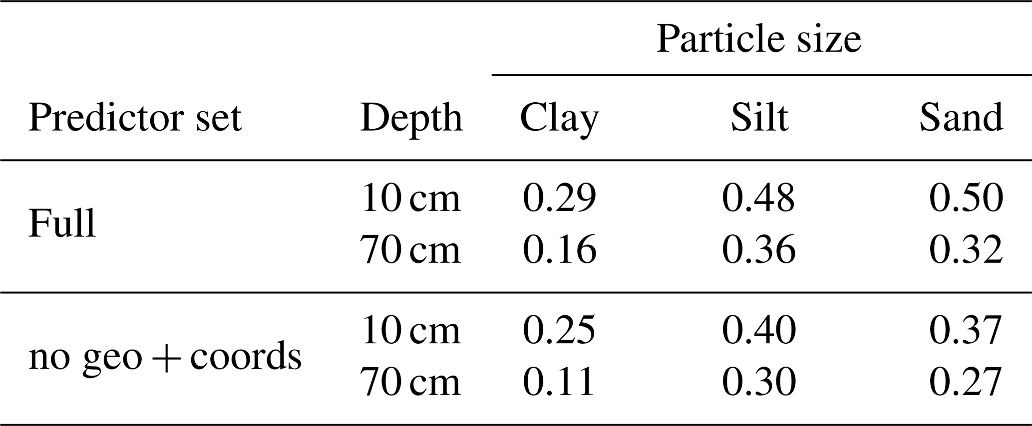
The R2 values for model performance of the full and no geo + coords models are shown in Table 3. Model performance of the silt and sand models at 10 cm depth are comparable to the results of Vaysse and Lagacherie (2015) and de Carvalho Junior et al. (2014), while other publications have shown that R2 values above 0.5 are achievable (Moore et al., 1993; Gobin et al., 2001; Adhikari et al., 2013). Moore et al. (1993) argue that R2 values above 0.7 are not to be expected due to the underlying random variability of soil and limitations in the accuracy of measurements. Differences in model performance are most likely to be related to the size and the heterogeneity of the study area and the quality of soil samples. This is illustrated well in Fig. 7, which demonstrates the variability of predictive performance across landscape types.
Table 3Model performance in R2 for three texture classes at two depth levels and for two predictor subsets.
3.2.2 Model specification
The mtry values for the full predictor model are shown in Fig. 9. There is no clear trend of optimal mtry value with model performance, and many models have a relatively large range of selected mtry values. It is worthwhile mentioning, though, that for certain models the selected mtry value is right at the lower boundary of the tested mtry parameter range, which is the case for the silt model at 10 cm. Accordingly, an extension of this lower boundary and the corresponding lower model complexity would likely have resulted in even better model performance.
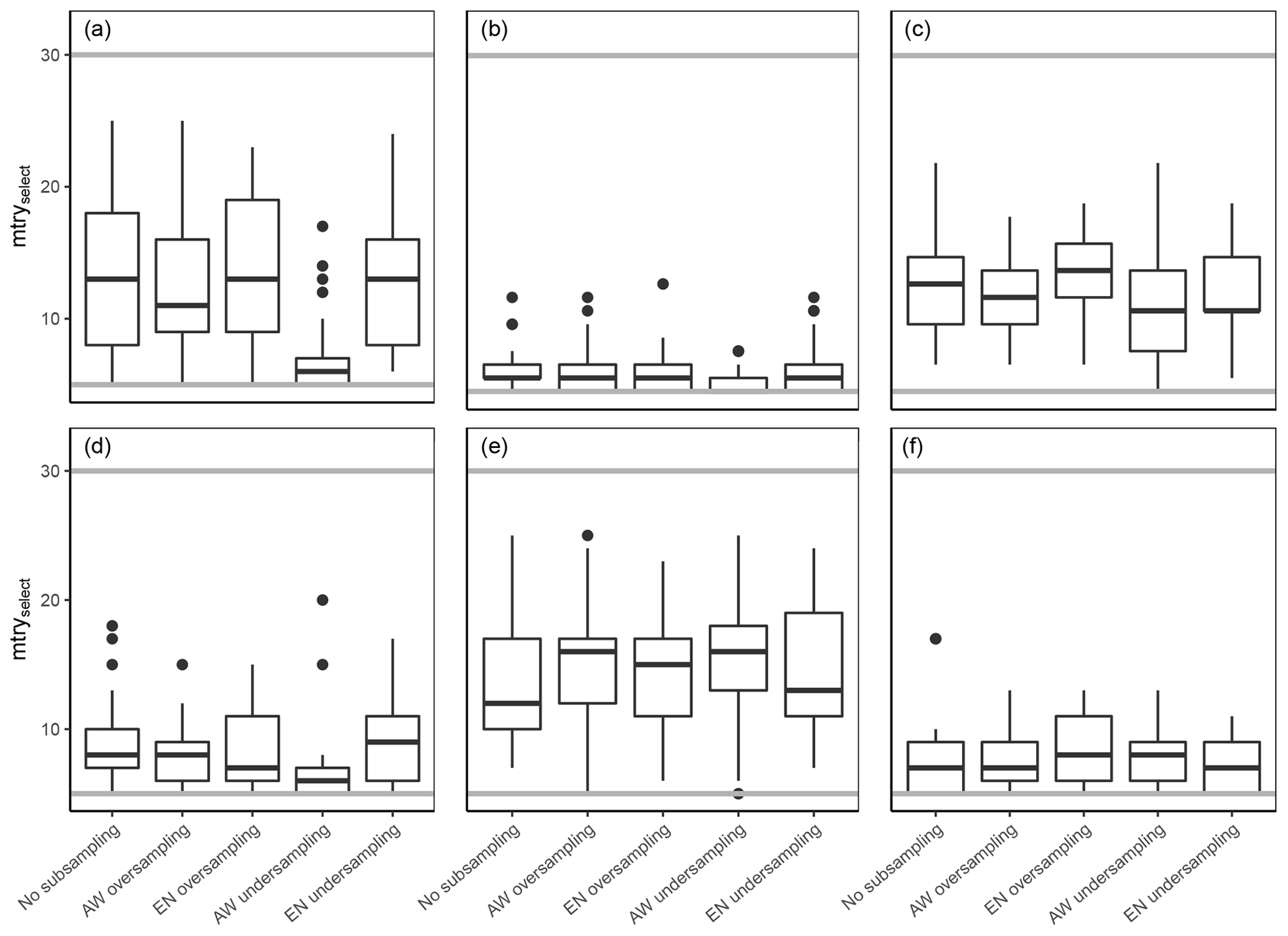
Figure 9Results of the model tuning procedure to find the best-performing mtry values (mtryselect) under different subsampling approaches. Panels (a), (b), and (c) show the results of the clay, silt, and sand models at 10 cm depth, while panels (d), (e), and (f) show the same texture classes at 70 cm depth. Grey lines correspond to the tested mtry parameter range.
Predictor importance is shown in Fig. 10a and b. The better model performance at 10 cm depth is reflected in the overall higher importance values. Altogether, petrography has the highest explanatory power. It should be noted, though, that GUEK 200 petrography was included for both depths, and GUEK 1000 petrography was only included in the model to predict soil texture at 10 cm depth (Table 2). There are few remaining predictors with notably increased predictive ability. These are latitude for silt and sand, positive openness, and the topographic ruggedness index (100 and 200 m radius) for sand and terrain surface texture (200 m radius) for clay.
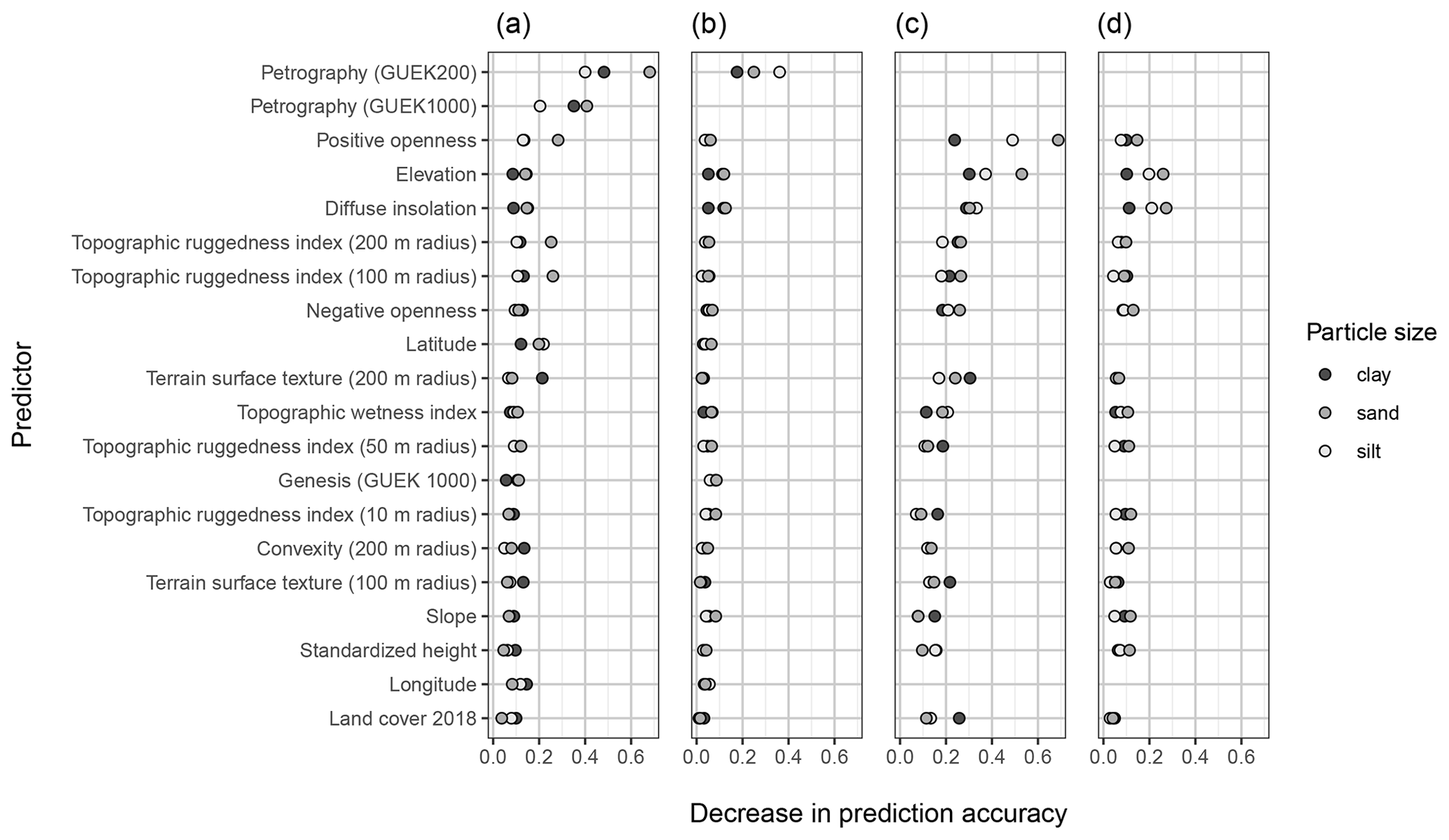
Figure 10Mean importance of the 20 strongest predictors of the model using the full predictor set (a, b) and the model leaving out the geologic maps and coordinates as predictors (c, d). Panels (a) and (c) show importance values for the models at 10 cm depth and panels (b) and (d) at 70 cm. Predictors are sorted by decreasing mean importance value. The importance metric is calculated as the decrease in prediction accuracy after the permutation of the predictor values.
Omitting the geologic information and coordinates leads to an overall increase in importance values for the remaining predictors (Fig. 10c). The importance value of elevation increased strongly. The same applies for many other topographical predictors, although in a less pronounced manner (positive and negative openness, diffuse insulation, terrain surface texture, 200 m radius).
3.3 Spatial prediction
Model output was generated by taking the median of all 25 models (CV procedure with five folds and five repetitions). The predicted, spatially continuous values of the sand, silt, and clay content at 10 cm depth corresponding to the models with the best median predictive performance (Fig. 6) are shown in Fig. 11. It needs to be noted that the maps of predicted values show the results of independent models for different soil texture classes, and the results do not add up to 100 %. The method to scale the data to 100 % should be selected with the purpose of the specific data utilization in mind. Different approaches could include leaving one of the texture classes out and summing up to 100 %, weighted scaling by texture class, or weighted scaling by the regional accuracy of the texture classes.
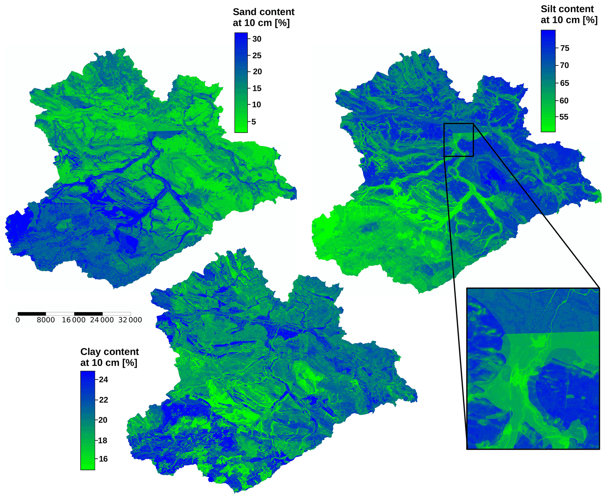
Figure 11Median of all predictions for sand, silt, and clay content at 10 cm depth. The maps show the output of the models built with the predictor set specified in Table 2. The scale bar shows distance in metres.
In the predicted spatial distribution of the sand and silt content, there is a strong regional difference between the lowlands and the mountainous region in the south-west. Sand content generally increases with elevation and is very high in riparian regions and valley bottoms. High silt contents can be expected in the lowlands outside riparian regions. The spatial variability of all three response variables is dominated by categorical predictor traits (petrography) that draw clear boundaries and even transfer artefacts present in the geological map products. However, it is more evident in the sand and clay model output. A limitation of the geologic maps, which is the lack of unity in the naming of geologic units between different geographic regions, but also at federal state boundaries for the GUEK 200, is also reproduced in the results. While the GUEK 1000 was generated by the German Federal Institute for Geosciences and Natural Resources (BGR), the GUEK 200 is a joint product between BGR and the regional geological survey institutions. Although the unit boundaries align across the map tiles, their description may differ because GUEK 200 harmonization at national level is not yet completed. This leads to an abrupt change in predicted sand and silt values in an otherwise homogeneous region (Fig. 11, areal zoom).
These model outputs clearly show the limitation in predictive capacity due to the limitations in the available data to represent the parent material. The prediction of soil texture is predominantly based on parent material, which allows us to distinguish the observed variability of soil texture between the lowlands and the mountains. Once parent material and coordinates are removed, the models increase the importance of those topographic predictors, which can be used to distinguish between these broad geographic regions (elevation, positive openness, diffuse insulation). Pedogenetic processes related to topography like the lateral redistribution of particles along slopes can only play a minor role, as the low importance values of predictors based on the immediate pixel neighbourhood have low importance values. However, other DSM approaches have successfully captured relief-based variability of soil texture on the scale of hillslopes using only topographical predictors (Moore et al., 1991; De Bruin and Stein, 1998; McBratney et al., 2000).
The inclusion of expert knowledge such as geological map products in machine learning models for the spatial continuous soil prediction at high resolution still requires further investigation. While the geologic maps have strong predictive power, they consist of too many geologic units. This leads to some units not having a sufficient number of soil samples to be able to generalize for that unit. However, our approach of reducing the number of geologic units by creating the particle size class bins was not able to produce useful predictors. One approach could be to use expert knowledge to merge geologic units that have parent material with similar soil texture classes. This merging should happen under the restriction that the resulting units should be as homogeneous as possible while providing enough samples for training and validation. Solving the issue of abrupt change in predicted values across geologic units could possibly be addressed by a fuzzy approach. Additionally, knowledge of the level of certainty of boundary demarcation between geologic units could be used to create fuzzy geologic maps as predictors.
In order to tackle the issue of artefacts present in the model output, two more models with a reduced set of predictors were built. The models using all predictors as specified in Table 2 (full) were compared to models leaving out the geologic predictors (no geo) or leaving out geology, latitude, and longitude (no geo + coords). Although the dominance of the categorical predictors on the model output was lifted in the “no geo” model version, an artefact due to the predictors longitude and latitude emerged. This new phenomenon appeared as a horizontal or vertical abrupt change in the predicted values across major parts of the study area (not shown). This aspect has already been observed in other DSM applications employing recursive partitioning algorithms (Behrens et al., 2018; Hengl et al., 2018; Nussbaum et al., 2018). Møller et al. (2020) addressed this problem with oblique geographic coordinates and provide an overview of ready applied approaches. Accordingly, we tested the usage of three Euclidean distance fields instead of Cartesian coordinates. However, the use of this alternative coordinate system led to the emergence of radial artefacts (results not shown).
The additional omission of latitude and longitude from the predictors leads to smoother maps, where only minor abrupt boundaries exist due to land cover, which is also a categorical predictor (Fig. 12). However, this aspect has to be differentiated from that of the geologic predictors. CORINE land cover classes were classified in remote sensing data products. Hence, spatial class boundaries do not reflect expert knowledge. Abrupt changes might in fact be due to land cover changes. The large agricultural fields of the lowlands are heavily impacted by wind erosion of the loess material during bare soil conditions. These “no geo + coords” predictions reproduce the spatial variability of the “full” model, even on relatively small scales. Strong deviations between the two model versions are in the eastern Harz region and in the riparian zones of the southern lowlands.
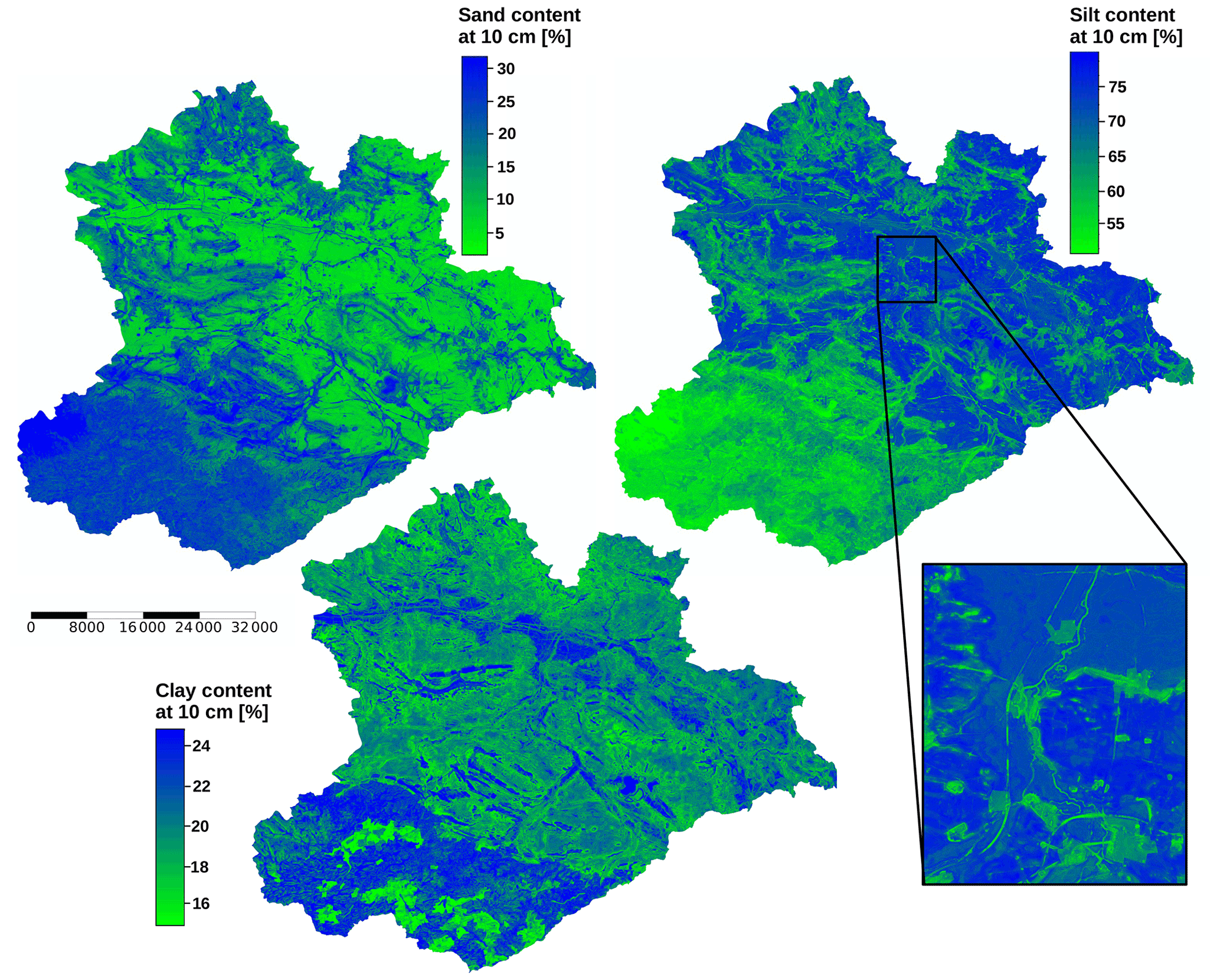
Figure 12Median of all predictions for sand, silt, and clay content at 10 cm depth. The maps show the output of the models built without using the geologic maps, longitude, and latitude as predictors. The scale bar shows distance in metres.
The differences in sand and silt content between the Harz and the lowlands were most likely derived from the predictors' elevation and positive openness. These predictors are strongly correlated (−0.95), have high importance values in both predictor sets, and show strong significant differences between the texture clusters (Fig. 5). The other predictors of Fig. 5 have lower values of absolute correlation with elevation (0.27–0.37) while still having a significant effect on the texture clusters. These predictors were more likely related to the variability within the two large-scale regions. The output of the “no geo + coords” models shows much more variability on smaller scales than the “full” models.
Our DSM approach has shown that RF is an appropriate method to model the variability of soil texture in the study area. The predictive performance of the silt and sand models is within the range of similar studies, while the prediction of the clay content did not seem feasible.
Clustering applications appear to be a versatile tool to be employed at various steps of the DSM procedure. Using a clustering application for feature selection offers additional insight into the predictor–response relationship, while clustering to conduct a stratified CV allowed for a robust model evaluation. Overall, stratified k-fold CV is common in DSM. To use the described cluster application allows for a simultaneous stratification regarding multiple response variables. However, to truly evaluate the power of this filter method, it would have to be compared to other feature selection methods which would have exceeded the workload for this study. We intend to do so in future studies.
The biggest area of application for data clustering in DSM appears to be in landscape stratification to divide the landscape into homogeneous subareas. Beyond their usage for stratified sampling and subsampling, the resulting stratification of the study area has further potential, like the use of landscape strata as predictors, the construction of individual models per landscape stratum, or the interpretation of the predictor–response relationship in different landscapes. A remaining difficulty in clustering applications is the determination of the number of clusters. Here, the combinations of clustering indices and heuristic methods have proven to be useful tools.
Finally, clustering applications could also provide solutions to the problems encountered during the model-building procedure, like the replacement of the Cartesian coordinates, the inclusion of expert knowledge, pooling of geologic units, and blurring of the transitions between geologic units.
The median predictions are available under https://doi.org/10.17605/OSF.IO/GMJTQ (Dunkl, 2022).
ML and ID conceived the study. ID performed the analysis and created the figures. ID and ML wrote the manuscript.
The contact author has declared that neither of the authors has any competing interests.
Publisher’s note: Copernicus Publications remains neutral with regard to jurisdictional claims in published maps and institutional affiliations.
The authors wish to thank the Landesamt für Geologie und Bergwesen of Saxony-Anhalt for providing the legacy dataset used for this study.
The article processing charges for this open-access publication were covered by the Helmholtz Centre for Environmental Research – UFZ.
This paper was edited by Bas van Wesemael and reviewed by two anonymous referees.
Adhikari, K., Kheir, R. B., Greve, M. B., Bøcher, P. K., Malone, B. P., Minasny, B., McBratney, A. B., and Greve, M. H.: High-resolution 3-D mapping of soil texture in Denmark, Soil Sci. Soc. Am. J., 77, 860–876, https://doi.org/10.2136/sssaj2012.0275, 2013. a, b, c
Behrens, T., Zhu, A.-X., Schmidt, K., and Scholten, T.: Multi-scale digital terrain analysis and feature selection for digital soil mapping, Geoderma, 155, 175–185, https://doi.org/10.1016/j.geoderma.2009.07.010, 2010. a, b
Behrens, T., Schmidt, K., Viscarra Rossel, R. A., Gries, P., Scholten, T., and MacMillan, R. A.: Spatial modelling with Euclidean distance fields and machine learning, Eur. J. Soil Sci., 69, 757–770, https://doi.org/10.1111/ejss.12687, 2018. a
Benjamini, Y. and Yekutieli, D.: The control of the false discovery rate in multiple testing under dependency, Ann. Stat., 29, 1165–1188, 2001. a
Beven, K. J. and Kirkby, M. J.: A physically based, variable contributing area model of basin hydrology, Hydrolog. Sci. J., 24, 43–69, https://doi.org/10.1080/02626667909491834, 1979. a
BGR: Geologische Karte der Bundesrepublik Deutschland 1 : 1.000.000 (GK1000 v4.0), Hannover, 2006. a
BGR: Geologische Übersichtskarte der Bundesrepublik Deutschland 1 : 200.000 (GÜK200), Hannover, 2007. a, b, c
BGR: Bodenübersichtskarte 1 : 200.000 (BÜK200 v1.5), Hannover, 2012. a
BKG: GeoBasis-DE, 2012. a
Blanco, C. M. G., Gomez, V. M. B., Crespo, P., and Ließ, M.: Spatial prediction of soil water retention in a Páramo landscape: Methodological insight into machine learning using random forest, Geoderma, 316, 100–114, https://doi.org/10.1016/j.geoderma.2017.12.002, 2018. a
Blume, H.-P., Brümmer, G. W., Horn, R., Kandeler, E., Kögel-Knabner, I., Kretzschmar, R., Stahr, K., and Wilke, B.-M.: Scheffer/schachtschabel: Lehrbuch der bodenkunde, Springer-Verlag, https://doi.org/10.1007/978-3-662-49960-3, 2016. a
Bock, M., Böhner, J., Conrad, O., Köthe, R., and Ringeler, A.: XV. Methods for creating Functional Soil Databases and applying Digital Soil Mapping with SAGA GIS, JRC Scientific and technical Reports, Office for Official Publications of the European Communities, Luxemburg, 2007. a
Böhner, J. and Antonić, O.: Land-surface parameters specific to topo-climatology, Dev. Soil Sci., 33, 195–226, https://doi.org/10.1016/S0166-2481(08)00008-1, 2009. a, b
Böhner, J. and Selige, T.: Spatial prediction of soil attributes using terrain analysis and climate regionalisation, Gottinger Geographische Abhandlungen, 115, 13–28, 2006. a, b, c, d, e, f
Breiman, L.: Random forests, Mach. Learn., 45, 5–32, https://doi.org/10.1023/A:1010933404324, 2001. a
Bulmer, C., Schmidt, M., Heung, B., Scarpone, C., Zhang, J., Filatow, D., Finvers, M., Berch, S., and Smith, S.: Improved soil mapping in British Columbia, Canada, with legacy soil data and random forest, in: Digital Soil Mapping Across Paradigms, Scales and Boundaries, edited by: Zhang, G.-L., Brus, D., Liu, F., Song, X.-D., and Lagacherie, P., 291–303, Springer, https://doi.org/10.1007/978-981-10-0415-5_24, 2016. a
Büttner, G., Feranec, J., Jaffrain, G., Mari, L., Maucha, G., and Soukup, T.: The CORINE land cover 2000 project, EARSeL eProceedings, 3, 331–346, 2004. a
Carré, F., McBratney, A. B., and Minasny, B.: Estimation and potential improvement of the quality of legacy soil samples for digital soil mapping, Geoderma, 141, 1–14, https://doi.org/10.1016/j.geoderma.2007.01.018, 2007. a
Chandrashekar, G. and Sahin, F.: A survey on feature selection methods, Comput. Electr. Eng., 40, 16–28, 2014. a
Charrad, M., Ghazzali, N., Boiteau, V., Niknafs, A., and Charrad, M. M.: Package “NbClust”, J. Stat. Softw., 61, 1–36, https://doi.org/10.18637/jss.v061.i06, 2014. a
Conrad, O., Bechtel, B., Bock, M., Dietrich, H., Fischer, E., Gerlitz, L., Wehberg, J., Wichmann, V., and Böhner, J.: System for Automated Geoscientific Analyses (SAGA) v. 2.1.4, Geosci. Model Dev., 8, 1991–2007, https://doi.org/10.5194/gmd-8-1991-2015, 2015. a, b, c, d, e
De Bruin, S. and Stein, A.: Soil-landscape modelling using fuzzy c-means clustering of attribute data derived from a digital elevation model (DEM), Geoderma, 83, 17–33, https://doi.org/10.1016/S0016-7061(97)00143-2, 1998. a
de Carvalho Junior, W., Lagacherie, P., da Silva Chagas, C., Calderano Filho, B., and Bhering, S. B.: A regional-scale assessment of digital mapping of soil attributes in a tropical hillslope environment, Geoderma, 232, 479–486, https://doi.org/10.1016/j.geoderma.2014.06.007, 2014. a, b
Deutscher Wetterdienst: Vieljährige Mittelwerte, https://www.dwd.de/DE/leistungen/klimadatendeutschland (last access: 22 August 2022), 2020. a
Dunkl, I.: Data set: On the benefits of clustering approaches in digital soil mapping: an application example concerning soil texture regionalization, OSF Home [data set], https://doi.org/10.17605/OSF.IO/GMJTQ, 2022. a
Evans, J. S., Murphy, M. A., Holden, Z. A., and Cushman, S. A.: Modeling species distribution and change using random forest, in: Predictive species and habitat modeling in landscape ecology, edited by: Drew, C. A., Wiersma, Y. F., and Huettmann, F., 139–159, Springer, https://doi.org/10.1007/978-1-4419-7390-0_8, 2011. a
Finnern, H., Grottenthaler, W., and Kühn, D.: Bodenkundliche Kartieranleitung (KA 4), 4. Verbesserte und erweiterte Auflage Hrsg., 1994. a, b
Friedrich, K.: Digitale Reliefgliederungsverfahren zur Ableitung bodenkundlich relevanter Flächeneinheiten, Fachbereich Geowiss. d. Johann-Wolfgang-Goethe-Univ., ISBN 9783922540557, 1996. a
Gobin, A., Campling, P., and Feyen, J.: Soil-landscape modelling to quantify spatial variability of soil texture, Phys. Chem. Earth Pt. B, 26, 41–45, https://doi.org/10.1016/S1464-1909(01)85012-7, 2001. a, b
Grunwald, S.: Multi-criteria characterization of recent digital soil mapping and modeling approaches, Geoderma, 152, 195–207, https://doi.org/10.1016/j.geoderma.2009.06.003, 2009. a
Grunwald, S., Thompson, J., and Boettinger, J.: Digital soil mapping and modeling at continental scales: Finding solutions for global issues, Soil Sci. Soc. Am. J., 75, 1201–1213, https://doi.org/10.2136/sssaj2011.0025, 2011. a, b
Guisan, A., Weiss, S. B., and Weiss, A. D.: GLM versus CCA spatial modeling of plant species distribution, Plant Ecol., 143, 107–122, 1999. a, b
Hamza, M. and Larocque, D.: An empirical comparison of ensemble methods based on classification trees, J. Stat. Comput. Sim., 75, 629–643, https://doi.org/10.1023/A:1009841519580, 2005. a
He, H. and Garcia, E. A.: Learning from imbalanced data, IEEE T. Knowl. Data En., 21, 1263–1284, https://doi.org/10.1109/TKDE.2008.239, 2008. a, b
Hengl, T., Nussbaum, M., Wright, M. N., Heuvelink, G. B., and Gräler, B.: Random forest as a generic framework for predictive modeling of spatial and spatio-temporal variables, PeerJ, 6, e5518, https://doi.org/10.7717/peerj.5518, 2018. a
Heung, B., Bulmer, C. E., and Schmidt, M. G.: Predictive soil parent material mapping at a regional-scale: A Random Forest approach, Geoderma, 214, 141–154, https://doi.org/10.1016/j.geoderma.2013.09.016, 2014. a, b
Heung, B., Ho, H. C., Zhang, J., Knudby, A., Bulmer, C. E., and Schmidt, M. G.: An overview and comparison of machine-learning techniques for classification purposes in digital soil mapping, Geoderma, 265, 62–77, https://doi.org/10.1016/j.geoderma.2015.11.014, 2016. a, b
Kalambukattu, J. G., Kumar, S., and Raj, R. A.: Digital soil mapping in a Himalayan watershed using remote sensing and terrain parameters employing artificial neural network model, Environ. Earth Sci., 77, 203, https://doi.org/10.1007/s12665-018-7367-9, 2018. a
Köthe, R. and Lehmeier, F.: SARA–System zur Automatischen Relief-Analyse, User Manual, 1996. a, b
Kuhn, M. and Johnson, K.: Applied predictive modeling, Vol. 26, Springer, ISBN 978-1-4614-6849-3, 2013. a, b
LAGB: Auszug aus der Bodenprofildatenbank (SABOP) mit Stand vom 12.05.2016, Landesamt für Geologie und Bergwesen Sachsen-Anhalt, 2018. a
Lê, S., Josse, J., and Husson, F.: FactoMineR: an R package for multivariate analysis, J. Stat. Softw., 25, 1–18, https://doi.org/10.18637/jss.v025.i01, 2008. a
Ließ, M.: Sampling for regression-based digital soil mapping: closing the gap between statistical desires and operational applicability, Spat. Stat., 13, 106–122, https://doi.org/10.1016/j.spasta.2015.06.002, 2015. a
Ließ, M.: At the interface between domain knowledge and statistical sampling theory: Conditional distribution based sampling for environmental survey (CODIBAS), Catena, 187, 104423, https://doi.org/10.1016/j.catena.2019.104423, 2020. a, b, c
Linting, M., Meulman, J. J., Groenen, P. J., and van der Kooij, A. J.: Nonlinear Principal Components Analysis: Introduction and Application, Psychol. Methods, 12, 336–358, https://doi.org/10.1037/1082-989X.12.3.336, 2007. a
MacMillan, R., Jones, R. K., and McNabb, D. H.: Defining a hierarchy of spatial entities for environmental analysis and modeling using digital elevation models (DEMs), Computers, Environment and Urban Systems, 28, 175–200, https://doi.org/10.1016/S0198-9715(03)00019-X, 2004. a
Marchi, L. and Dalla Fontana, G.: GIS morphometric indicators for the analysis of sediment dynamics in mountain basins, Environ. Geol., 48, 218–228, https://doi.org/10.1007/s00254-005-1292-4, 2005. a
McBratney, A. B., Odeh, I. O., Bishop, T. F., Dunbar, M. S., and Shatar, T. M.: An overview of pedometric techniques for use in soil survey, Geoderma, 97, 293–327, https://doi.org/10.1016/S0016-7061(00)00043-4, 2000. a
McBratney, A. B., Santos, M. M., and Minasny, B.: On digital soil mapping, Geoderma, 117, 3–52, https://doi.org/10.1016/S0016-7061(03)00223-4, 2003. a, b
Minasny, B. and McBratney, A. B.: Digital soil mapping: A brief history and some lessons, Geoderma, 264, 301–311, https://doi.org/10.1016/j.geoderma.2015.07.017, 2016. a
Møller, A. B., Beucher, A. M., Pouladi, N., and Greve, M. H.: Oblique geographic coordinates as covariates for digital soil mapping, SOIL, 6, 269–289, https://doi.org/10.5194/soil-6-269-2020, 2020. a
Moore, I. D., Grayson, R., and Ladson, A.: Digital terrain modelling: a review of hydrological, geomorphological, and biological applications, Hydrol. Process., 5, 3–30, https://doi.org/10.1002/hyp.3360050103, 1991. a, b
Moore, I. D., Gessler, P., Nielsen, G., and Peterson, G.: Soil attribute prediction using terrain analysis, Soil Sci. Soc. Am. J., 57, 443–452, https://doi.org/10.2136/sssaj1993.03615995005700020026x, 1993. a, b
Moran, C. J. and Bui, E. N.: Spatial data mining for enhanced soil map modelling, Int. J. Geogr. Inf. Sci., 16, 533–549, https://doi.org/10.1080/13658810210138715, 2002. a, b
Nussbaum, M., Spiess, K., Baltensweiler, A., Grob, U., Keller, A., Greiner, L., Schaepman, M. E., and Papritz, A.: Evaluation of digital soil mapping approaches with large sets of environmental covariates, SOIL, 4, 1–22, https://doi.org/10.5194/soil-4-1-2018, 2018. a
OpenStreetMap contributors: Planet dump, https://planet.osm.org and https://www.openstreetmap.org (last access: 20 February 2019), 2018. a
Padarian, J., Minasny, B., and McBratney, A. B.: Machine learning and soil sciences: a review aided by machine learning tools, SOIL, 6, 35–52, https://doi.org/10.5194/soil-6-35-2020, 2020. a
Park, S. and Vlek, P.: Environmental correlation of three-dimensional soil spatial variability: a comparison of three adaptive techniques, Geoderma, 109, 117–140, https://doi.org/10.1016/S0016-7061(02)00146-5, 2002. a, b
Peel, M. C., Finlayson, B. L., and McMahon, T. A.: Updated world map of the Köppen-Geiger climate classification, Hydrol. Earth Syst. Sci., 11, 1633–1644, https://doi.org/10.5194/hess-11-1633-2007, 2007. a
R Core Team: R: A Language and Environment for Statistical Computing, R Foundation for Statistical Computing, Vienna, Austria, http://www.R-project.org/ (last access: 18 August 2022), 2018. a
Riley, S. J.: Index that quantifies topographic heterogeneity, Intermountain Journal of Sciences, 5, 23–27, 1999. a, b
Rossiter, D. G.: Past, present & future of information technology in pedometrics, Geoderma, 324, 131–137, https://doi.org/10.1016/j.geoderma.2018.03.009, 2018. a
Schmidt, K., Behrens, T., and Scholten, T.: Instance selection and classification tree analysis for large spatial datasets in digital soil mapping, Geoderma, 146, 138–146, https://doi.org/10.1016/j.geoderma.2008.05.010, 2008. a
Schubert, E. and Zimek, A.: ELKI: A large open-source library for data analysis-ELKI Release 0.7.5 “Heidelberg”, arXiv [preprint], https://doi.org/10.48550/arXiv.1902.03616, 2019. a
Scull, P., Franklin, J., Chadwick, O., and McArthur, D.: Predictive soil mapping: a review, Prog. Phys. Geogr., 27, 171–197, https://doi.org/10.1191/0309133303pp366ra, 2003. a, b
Sharififar, A., Sarmadian, F., Malone, B. P., and Minasny, B.: Addressing the issue of digital mapping of soil classes with imbalanced class observations, Geoderma, 350, 84–92, https://doi.org/10.1016/j.geoderma.2019.05.016, 2019. a, b
Subburayalu, S. K. and Slater, B. K.: Soil series mapping by knowledge discovery from an Ohio county soil map, Soil Sci. Soc. Am. J., 77, 1254–1268, https://doi.org/10.2136/sssaj2012.0321, 2013. a
Taghizadeh-Mehrjardi, R., Schmidt, K., Eftekhari, K., Behrens, T., Jamshidi, M., Davatgar, N., Toomanian, N., and Scholten, T.: Synthetic resampling strategies and machine learning for digital soil mapping in Iran, Eur. J. Soil Sci., 71, 352–368, https://doi.org/10.1111/ejss.12893, 2019. a
TGL: TGL 24300 Aufnahme landwirtschaftlich genutzter Standorte., Fachbereichsstandards, Akademie der Landwirtschaftswissenschaften der DDR, Berlin, 1985. a
Vaysse, K. and Lagacherie, P.: Evaluating digital soil mapping approaches for mapping GlobalSoilMap soil properties from legacy data in Languedoc-Roussillon (France), Geoderma Regional, 4, 20–30, https://doi.org/10.1016/j.geodrs.2014.11.003, 2015. a, b
Vaysse, K. and Lagacherie, P.: Using quantile regression forest to estimate uncertainty of digital soil mapping products, Geoderma, 291, 55–64, https://doi.org/10.1016/j.geoderma.2016.12.017, 2017. a, b
Wang, L. and Liu, H.: An efficient method for identifying and filling surface depressions in digital elevation models for hydrologic analysis and modelling, Int. J. Geogr. Inf. Sci., 20, 193–213, https://doi.org/10.1080/13658810500433453, 2006. a
Were, K., Bui, D. T., Øystein B. Dick, and Singh, B. R.: A comparative assessment of support vector regression, artificial neural networks, and random forests for predicting and mapping soil organic carbon stocks across an Afromontane landscape, Ecol. Indic., 52, 394–403, https://doi.org/10.1016/j.ecolind.2014.12.028, 2015. a
Yokoyama, R., Shirasawa, M., and Pike, R. J.: Visualizing topography by openness: a new application of image processing to digital elevation models, Photogramm. Eng. Rem. S., 68, 257–266, 2002. a, b
Zacharias, S., Bogena, H., Samaniego, L., Mauder, M., Fuß, R., Pütz, T., Frenzel, M., Schwank, M., Baessler, C., Butterbach-Bahl, K., Bens, O., Borg, E., Brauer, A., Dietrich, P., Hajnsek, I., Helle, G., Kiese, R., Kunstmann, H., Klotz, S., Munch, J. C., Papen, H., Priesack, E., Schmid, H. P., Steinbrecher, R., Rosenbaum, U., Teutsch, G., and Vereecken, H.: A network of terrestrial environmental observatories in Germany, Vadose Zone J., 10, 955–973, https://doi.org/10.2136/vzj2010.0139, 2011. a
Zevenbergen, L. W. and Thorne, C. R.: Quantitative analysis of land surface topography, Earth Surf. Proc. Land., 12, 47–56, https://doi.org/10.1002/esp.3290120107, 1987. a
Zhao, Z., Chow, T. L., Rees, H. W., Yang, Q., Xing, Z., and Meng, F.-R.: Predict soil texture distributions using an artificial neural network model, Comput. Electron. Agr., 65, 36–48, https://doi.org/10.1016/j.compag.2008.07.008, 2009. a
Zhou, Y., Hartemink, A. E., Shi, Z., Liang, Z., and Lu, Y.: Land use and climate change effects on soil organic carbon in North and Northeast China, Sci. Total Environ., 647, 1230–1238, https://doi.org/10.1016/j.scitotenv.2018.08.016, 2019. a