the Creative Commons Attribution 4.0 License.
the Creative Commons Attribution 4.0 License.
 | 06 Jul 2021
Predicting the spatial distribution of soil organic carbon stock in Swedish forests using a group of covariates and site-specific data
Kpade O. L. Hounkpatin
Johan Stendahl
Mattias Lundblad
Erik Karltun
The status of the soil organic carbon (SOC) stock at any position in the landscape is subject to a complex interplay of soil state factors operating at different scales and regulating multiple processes resulting either in soils acting as a net sink or net source of carbon. Forest landscapes are characterized by high spatial variability, and key drivers of SOC stock might be specific for sub-areas compared to those influencing the whole landscape. Consequently, separately calibrating models for sub-areas (local models) that collectively cover a target area can result in different prediction accuracy and SOC stock drivers compared to a single model (global model) that covers the whole area. The goal of this study was therefore to (1) assess how global and local models differ in predicting the humus layer, mineral soil, and total SOC stock in Swedish forests and (2) identify the key factors for SOC stock prediction and their scale of influence.
We used the Swedish National Forest Soil Inventory (NFSI) database and a digital soil mapping approach to evaluate the prediction performance using random forest models calibrated locally for the northern, central, and southern Sweden (local models) and for the whole of Sweden (global model). Models were built by considering (1) only site characteristics which are recorded on the plot during the NFSI, (2) the group of covariates (remote sensing, historical land use data, etc.) and (3) both site characteristics and group of covariates consisting mostly of remote sensing data.
Local models were generally more effective for predicting SOC stock after testing on independent validation data. Using the group of covariates together with NFSI data indicated that such covariates have limited predictive strength but that site-specific covariates from the NFSI showed better explanatory strength for SOC stocks. The most important covariates that influence the humus layer, mineral soil (0–50 cm), and total SOC stock were related to the site-characteristic covariates and include the soil moisture class, vegetation type, soil type, and soil texture. This study showed that local calibration has the potential to improve prediction accuracy, which will vary depending on the type of available covariates.
- Article
(6491 KB) - Full-text XML
-
Supplement
(4163 KB) - BibTeX
- EndNote


About 30 % of the global terrestrial carbon (C) stock is stored in forests, with 60 % located belowground (Pan et al., 2011). These forests act mostly as a large net sink for atmospheric carbon, but concerns exist for the potential release of C under the impact of global warming over the next century (Price et al., 2013; Kauppi et al., 2014). Moreover, the intensification of forest management for timber, fibre, and fuel to satisfy an ever-increasing demand will likely affect the dynamic of the forest C pool. In recent decades, many studies have focused on assessing the soil organic carbon (SOC) stock in forest soils (Kumar et al., 2016; Ottoy et al., 2017; Sheikh et al., 2009; Prietzel and Christophel, 2014), which is crucial for meeting the requirements of the climate convention and the Kyoto Protocol for reporting all sources and sinks of carbon dioxide and also for estimating potential carbon credits (Buchholz et al., 2014; Jandl et al., 2007). In that context, analysis of the C cycle in forests is crucial to the understanding of climate-related changes in the global C pool.
The increased availability of remote sensing data and development of spatial statistical methods has led to an increased use of digital soil mapping (DSM; Minasny and McBratney, 2016). DSM aims at estimating the spatial distribution of soil classes or soil properties by coupling field and laboratory observations with spatial and non-spatial environmental covariates via quantitative relationships. Many studies used DSM approaches to predict the SOC stock at different scales and for various land use/land cover, climate, and also across a wide range of soil types (Söderström et al., 2016; Tranter et al., 2011; Beguin et al., 2017; Mansuy et al., 2014; Mallik et al., 2020). These studies use different modelling techniques ranging from geostatistics and multiple linear regression to machine learning models such as artificial neural networks, support vector machines, and boosted regression trees.
The accuracy and precision of predictions resulting from modelling over a large extent are often reported to be poor because of the spatial heterogeneity encompassing different soil types, topography, and soil properties (Grimm et al., 2008; Schulp and Verburg, 2009; Schulp et al., 2013; Tang et al., 2017). Generally, models are applied to the whole study area without prior stratification. However, models could be calibrated separately for sub-areas, and their predictions can then be combined to cover the whole area (Somarathna et al., 2016; Piikki and Söderström, 2019; Song et al., 2020). Since spatial variability is an important characteristic of forest landscapes, key drivers of SOC stock might be specific for sub-areas compared to those influencing the whole landscape. Management decisions in relation to the driving factors of the SOC stock will likely be more cost-effective as models gain in reliability for specific areas within a given landscape.
Building on the soil state factor (climate, organisms, relief, parent material, and age) equation developed by Jenny (1941), McBratney et al. (2003) introduced the conceptual framework for DSM referred to as SCORPAN, which complemented the former with the inclusion of soil information and location coordinates. The relative contribution of any of these factors to the model accuracy in DSM varies, and some turn out to be more relevant as explanatory covariates compared to others. Ottoy et al. (2017) identified relief (highest groundwater level), soil (clay fraction), and land use (tree genus) as being the main predictors for mapping SOC stock in forest soils in Belgium, while Mansuy et al. (2014) reported relief and climatic covariates as being the key covariates in mapping C, N, and texture in Canadian managed forests. Vasques et al. (2016) recorded parent material among the key covariates in mapping soil properties in a tropical dry forest in Brazil. These studies and many others rely mostly on covariates existing as maps, while survey data, which present site-specific information, are left out during modelling. However, soil factors affecting different processes in the landscape operate at different scales, and taking into account site-specific covariates would inform model local variability, which might not be captured by remote sensing covariates.
The goal of this study was therefore to (1) assess how global and local models differ for predicting the humus layer, mineral soil, and total SOC stock in Sweden forest ecosystems, (2) evaluate to which extent and at which scale remotely sensed covariates can explain the variability in SOC stock compared to site-specific covariates in the Swedish forest, and (3) identify covariates which may have potential for future prediction models in forest SOC stock assessments.
2.1 Data description
Forest data came from the Swedish National Forest Soil Inventory (NFSI) and the National Forest Inventory (NFI). The NFSI runs concurrently every year with the NFI and consists of repeated surveys of forest vegetation and soil chemical and physical properties (Stendahl et al., 2017; Ortiz et al., 2013). Data from the following inventory periods were considered in the present study: 1993–2002, 2003–2012, and 2013–2015. However, the present paper did not focus on SOC changes over these three inventory periods but on SOC stock using plot scale as a unit. The NFSI are conducted on ca. 23 500 permanent plots (Fig. 1), with a radius of 10 m, covering all land uses in Sweden except urban areas, cultivated land, and the high mountains. The plots are distributed based on a stratified and random national grid system covering all the Swedish forest soils. They are organized in quadratic clusters (tracts) consisting of eight (in the north) to four (in the southwest) circular (314 m2) sample plots. Each plot of the NFSI is inventoried once every 10 years.
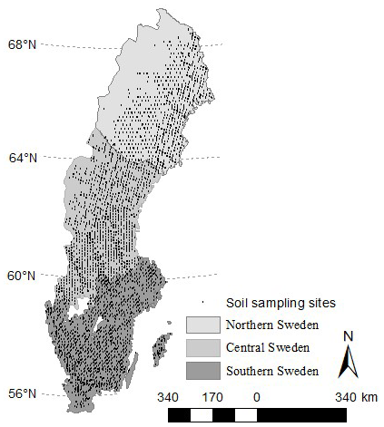
Figure 1Sites from the Swedish Forest Soil Inventory for northern, central, and southern Sweden.
Soil samples are collected in a subset of the plots, with humus sampling on ca. 10 000 plots and mineral soil sampling on ca. 4500 plots (Stendahl et al., 2017). Based on the NFSI data set, pedogenetic carbonates are not formed in these soils due to sufficient leaching and also sedimentary bedrocks, which could potentially contain CaCO3, cover less than 1 % of Swedish forests. Therefore, the content of inorganic carbon in mineral soil is considered negligible in the study area. Humus layer volumetric samples are taken using a soil core (core diameter 10 cm) below the O horizon down to 30 cm depth. The mineral soil is sampled at 0–10, 10–20, and 55–65 cm depth from the mineral soil surface. These samples are dried at 35 ∘C and sieved to <2 mm. Total C is determined for all samples by dry combustion with elemental analysers (LECO CNS-1000 and LECO TruMac CN). Total O horizon SOC stock is calculated from the sampled amount of soil material and the C concentration of the sample. The total mineral SOC stock down to 50 cm depth for each site is calculated using the SOC stock of measured layers with the empirical model for bulk density (Nilsson and Lundin, 2006), corrections for stoniness (Stendahl et al., 2009), and linear interpolation between measured layers. Since the potential SOC stock change is very small compared to the entire SOC stock, the averaged SOC stock between the inventories was considered representative of the plots and was, therefore, considered for all computations and modelling in order to the reduce variability between plots. The organic and mineral soil SOC stock were summed up to obtain the total SOC stock.
2.2 Explanatory covariates for prediction
The set of covariates used in this study consist of topographic covariates, climate covariates, geochemical and gamma ray data, historical land use maps, and site characteristics (Table 1).
Table 1List of explanatory covariates for predicting SOC stock.
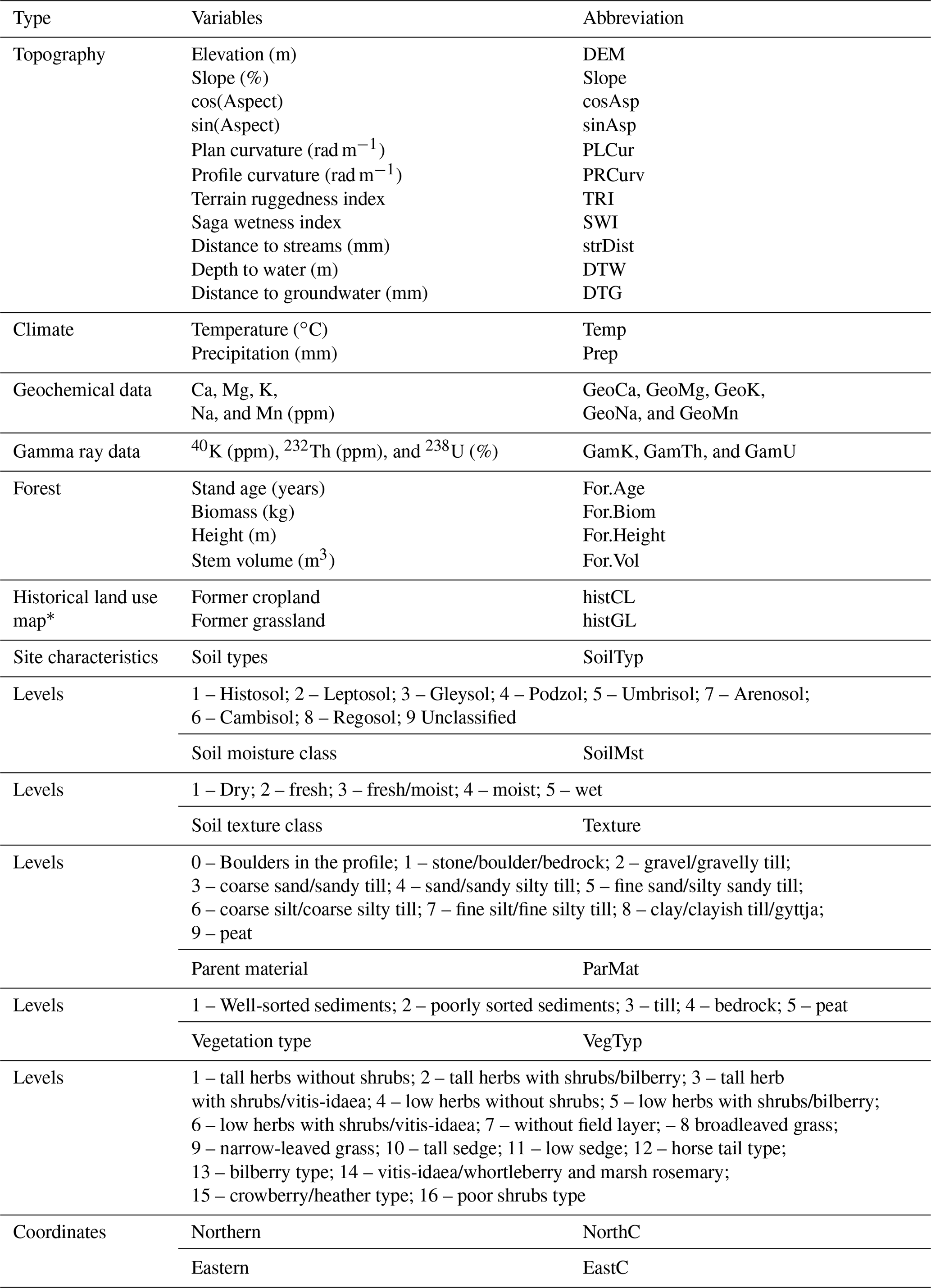
* Used only for the southern part of Sweden.
Topographic covariates were computed from high-resolution digital elevation models (DEMs) derived from light detection and ranging (lidar) produced by the Swedish National Mapping Agency. It was originally created with 2 m spatial resolution (Dowling et al., 2013). However, the initial DEM was resampled in the ArcGIS 10 software package using the aggregation procedure with bilinear interpolation to a final resolution of 10 m × 10 m, which is reasonable for the data considered in the present study. The topographical covariates were computed using the SAGA GIS software (Conrad et al., 2015). However, the depth to water (DTW; 2 × 2 m) considered in this study is an estimation of the elevation along a defined least cost path (Lidberg et al., 2019; Murphy et al., 2008). The depth to groundwater was obtained from the Swedish Forest Agency (SGU, 2018) and computes the difference in elevation in relation to surrounding cells following the vertical flow path.
Climate maps (1 km × 1 km) of the annual mean temperature and annual precipitation for 1970–2000 were obtained from the WorldClim platform (Fick and Hijmans, 2017). The Geological Survey of Sweden (SGU) has produced geochemical data based mainly on the spatial distribution of till which covers about 75 % of the Swedish landscape. The following base cations Ca (parts per million; hereafter ppm), Mg (ppm), K (ppm), Na (ppm) and Mn (ppm) were considered for the present study in predicting carbon storage (Andersson et al., 2014).
Several studies in Sweden pointed to some correlation between gamma ray data and soil properties (Piikki et al., 2015; Söderström and Eriksson, 2013). Gamma ray data have been recorded by SGU since 1968, with measurements carried out along flight lines at 200 m intervals in general. The flight heights were 30 m up to 1994, while subsequent surveys were carried out at 60 m altitude. The concentrations of the following radioisotopes 40K, 232Th, and 238U are measured and corrected for background and cosmic radiation (Erdi-Krausz et al., 2003). The gamma ray data set was filtered for values < 0, which were omitted as they are mostly related to water entities. The resulting gamma ray data and the geochemical data were interpolated in this study into maps either by ordinary kriging or inverse distance weighing when geostatistic assumptions, such as normal distribution, were not met.
The Swedish Forest Agency has developed several forest attributes maps based on the combination of satellite images and field data from the NFI (Nilsson et al., 2017). Maps (25 × 25 m) of the stand age, tree biomass, tree height, and stem volume produced for the year 2010 were used in the present study. Auffret et al. (2017a) digitized some historical map series (Ekonomiska kartan) which were initially published in 1935–1978. The digitized versions of these maps (1 × 1 m) were only produced for the southern part of Sweden and present past major land use, settlements, and infrastructure. These maps were available per county but were merged into a single raster file in ArcMap 10.7. For the present study, we consider two variants of these maps, i.e. (1) areas which were cropland and are now forest lands and (2) areas which were grasslands and are now forest lands.
The records of site characteristics (Table 1) are also carried out during the NFSI. The site description includes soil types, soil moisture class, soil texture class, vegetation type, and parent material class. The soil classification was based on the World Reference Base (WRB) for soil resources. The location of the average groundwater table over the vegetation season was the main criterion for defining classes of soil moisture. The texture index was made by manual assessment in the field, e.g. through the rolling and washing test. The vegetation type, as reported in Table 1, was defined by combining the descriptions of the field layers which refer to the understorey. Field layers consisted of four main types which are categorized from fertile to poor, namely herb types (tall or low), grounds without field layer, grass types, and dwarf shrub types.
2.3 Prediction models: random forest and quantile regression forest
The random forest (RF) algorithm was selected for SOC stock prediction. Additionally, the quantile regression forest (QRF) was used to estimate the standard deviation related to the predictions.
RF is a classification and regression method that builds multiple decision trees. For regression, the tree predictors provide numerical output instead of class labels for classification (Breiman, 2001). The RF is able to model complex and nonlinear relationships between input predictors and response covariates. The RF is characterized by double randomness in the construction of the decisions trees. An ensemble of growing decision trees is generated by combining bagging (bootstrap aggregating) along with random feature selection. Bagging consists of producing training data sets (bootstrap sample) by drawing randomly with replacement from the original training data set generated. A regression tree is fitted to each of the bootstrap samples from a random subset of the input predictors when deciding to split a node. For any new given input X=x, RF provides the prediction of a single tree as a weighted average of the original observations Yi () in each node.
where wi is the weight vector which results either in a positive constant when the observation (Yi,Xi) is inherent to the leaf generated from the random vector of covariates or is 0 if otherwise. The weight vector (Meinshausen, 2006) wi is defined as follows:
Rl(x,θ) is the rectangular subspace defined by the leaf l(x,θ) of the tree built from the random vector of covariates θ and the input xi and xj (). The conditional mean is computed by averaging the predictions of k single trees which are individually built with independent vectors having similar distributions. The weighted average of trees is computed as follows:
The final prediction of the RF regression is given by the following:
The number of trees to grow in the RF model (ntree) and the number of randomly selected predictor covariates at each node (mtry) are the two key parameters to be tuned for RF modelling. To reduce computational load, the ntree was set at 500 while the mtry was tuned using the grid search (2 – p, with p being the number of covariates) method in the R caret package (Kuhn, 2015) with 50-fold cross validation. The importance of each input predictor can be assessed by the RF based on the mean decrease accuracy (MDA; Hastie et al., 2011). The MDA is computed by (i) randomly permuting the values of each predictor within the out of bag sample and (ii) measuring the reduction in model accuracy resulting from that permutation. The hypothesis is that this permutation would result in little to no effect on model accuracy for less important covariates, while significant drop will follow the permutation of important covariates.
2.4 Covariate layers processing for sub-areas
We considered three sub-areas in Sweden (Fig. 1) which are hereafter reported as northern (north), central (centre), and southern (south) Sweden areas in the remainder of the paper. These areas were defined by merging the northern, central, and southern climatic regions which were considered in Ortiz et al. (2013). A buffer of 4 km was considered for the shapefiles of each sub-area to create overlapping zones which ensured smooth transition while merging by averaging the SOC stock values within these shared units. The covariates were delimited for each sub-area. They were resampled to 10 m resolution using the bilinear method for continuous covariates and the nearest neighbour method for categorical covariates. A value to point extraction was carried out by overlaying the coordinates of the sampling points of each sub-areas over the stacked raster files in R (Kuhn, 2015). The pixel values of each sub-area were compiled to form the database of the humus layer and mineral and total SOC stock.
2.5 Modelling with different category of covariates: global and local models
For modelling, the following three categories of covariates were considered: (1) only the plot-level, site-specific covariates (SSCs), (2) all the covariates without the SSC, namely the group of covariates (GoCs), and (3) both the SSCs and GoCs (allCs). Modelling with RF was carried out with each category of covariate related to its sub-areas and for the compiled data set for the whole of Sweden. Moreover, to reduce computation time while keeping relatively the same level of accuracy, we (1) used feature preprocessing capabilities implemented in the caret package (Kuhn, 2019) of R to remove highly correlated (Pearson's correlation) expressions, using a cutoff point of 0.80, and (2) the recursive feature elimination (RFE) using RF as a method to select the optimal set of covariates for each RF model. The RFE functions by carrying out a variable importance classification then proceeds by iteratively eliminating the least important features (Gomes et al., 2019; Hounkpatin et al., 2018). For each RF model, the RFE was carried out, and therefore, the model-specific optimal set of covariates were identified for both sub-areas and the whole of Sweden.
Table 2Descriptive statistics for the training and validation data sets.
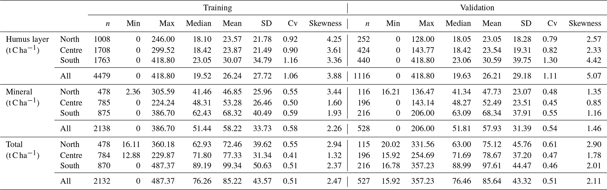
The RF models built on data covering the whole area of Sweden are hereafter called global models. The RF models created for each of the sub-areas are hereafter reported as local models. Considering the sub-areas as strata, the local models were built by randomly splitting the local data sets into calibration (80 %) and validation (20 %) subsets (Table 2). Each local model was validated against their respective local validation set. For comparison, the global models were validated using the same local validation set used for the local models. The data used for calibrating the global model was made up of the 80 % random split of the three local training sets (northern, central, and southern training sets). The same approach is used for validation at a national scale by considering as one data set the 20 % split of the three local validation data sets (northern, central, and southern validation sets). We trained both global and local models based on 10-fold cross-validation with five repetitions using the R caret package (Kuhn, 2015).
2.6 Assessment of model performance and mapping
To compare model performance, we computed several assessment metrics, i.e. R2, Lin's concordance (Lawrence and Lin, 1989) correlation (ρc), root mean square error (RMSE) and mean absolute error (MAE), and the bias.
where P is the predicted value, O is the observed/true value, μobs and μpred are the means of the observed and predicted values, respectively, and are the associated variances, and ρ is the correlation between the observed and the predicted values.
Though these error metrics are widely used for assessing models, they cannot inform about the uncertainty related to the prediction. Therefore, we additionally considered the density distribution of the predicted versus actual SOC stock. Furthermore, the scattergram of the prediction interval coverage probability (PICP) was also considered (Vaysse and Lagacherie, 2017). The latter is the graphical representation of the proportion of time the actual values of SOC stock fall within a series of probability (p) of prediction intervals (PI) limited by and quantiles. The QRF was used to predict all percentiles, including the 5th and 95th percentile required to create the 90 % prediction intervals. Finally, the coverage of the 90 % prediction intervals by the observation from the validation set was also analysed.
The SOC stock maps were computed only for the models based on the GoC models because of their availability as maps. The uncertainty in the SOC stock predictions was expressed by considering the coefficient of variation which is the percentage ratio of the standard deviation map divided by the mean SOC stock prediction. A qualitative assessment of the spatial distribution of the humus layer, mineral soil, and total SOC stock from the produced maps was carried out and compared to literature.
3.1 Validation performance of global models over the whole of Sweden
The performance metrics of the cross- and independent validation of the RF models at the national scale are presented in Table 3. The internal accuracy statistics showed that modelling with all covariates generally resulted in marginally lower RMSE and higher R2 for all SOC stock. Modelling with allCs reduced the cross-validation RMSE by 2 %, 1 %, and 6 % compared to SSC models and by 7.9 %, 10 %, and 6 % compared to GoC models, respectively, for the humus layer, mineral soil, and total SOC stock. Though modelling with allCs resulted in higher cross-validation R2 compared to the remaining models, only 30 %, 29 %, and 28 % of the total variance were explained, respectively, for the total SOC stock, mineral soil, and the humus layer SOC stock.
Table 3Cross-validation and independent validation of the global random forest models at the national scale.
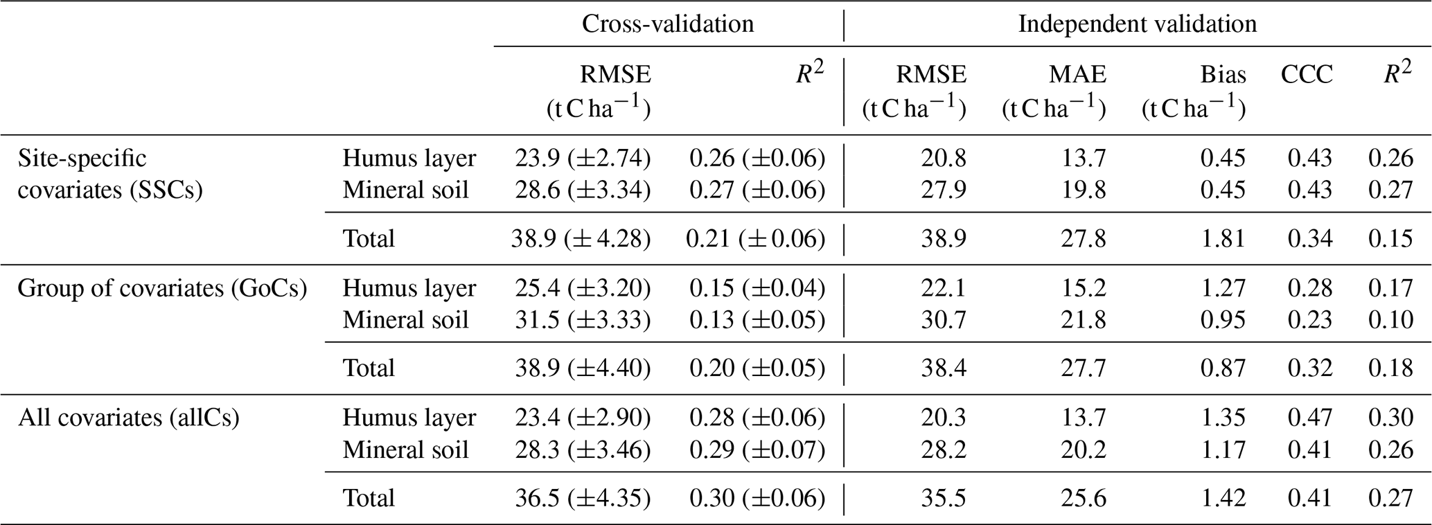
RMSE – root mean square error; MAE – mean absolute error; CCC – Lin's correlation concordance coefficient; R2 – coefficient of determination.
The independent validation showed similar trends as observed for the cross-validation. The Lin's correlation concordance coefficient (CCC) confirmed that the predictive performance of RF for the different SOC stock was enhanced either by using only SSCs or allCs. The similarity between the RMSE values of both training and validation data shows that the global models over Sweden did no overfit. However, the explained variances are as low as for the cross-validation varying from 15 % to 27 % for the SSC models, 10 % to 18 % for the GoC models, and from 26 % to 30 % for the allC models. For both cross- and independent validation, the RMSE increased with depth, with the lowest values recorded for the humus layer.
3.2 Validation performance of local models versus global models
As observed for the global models at the national scale, better accuracy was recorded for the local models based on allCs and SSCs, which present, in general, lower RMSE and higher CCC and R2 when compared to the local GoC models for the cross-validation (Table 4). The cross-validation with the local models resulted in lower RMSE compared to the values recorded for the global models (Table 3), except for the southern Sweden models which recorded higher values regardless of the category of covariates. Local models with allC reduced the RMSE of cross-validation in relation to the global models (Table 3) by 18 % for both northern and central Sweden for the humus layer SOC stock, by 21 % (north) and 20 % (centre) for the mineral soil SOC stock, and by 9 % (north) and 24 % (central) for the total SOC stock. The variances explained by the local models based on cross-validation varied from 17 % to 32 % for allC models, 12 % to 25 % for the SSC models, and from 5 % to 20 % for the GoC models.
Table 4Cross-validation of the local random forest models.

RMSE – root mean square error; R2 – coefficient of determination.
The global models were also used to make predictions with the same independent validation set used for the local models. Though the local models generally outperformed the global models, the results were different based on the sub-areas and category of covariates (Fig. 2). However, the local SSC models were more consistent at outperforming the global SSC models compared to GoC and allC models when tested with an independent data set. For the humus layer (Fig. 2a) and the mineral (Fig. 2b) and total soil layers (Fig. 2c), the local models had, in general, better performance than the global models in term of RMSE within each set of variables. The best local models were mostly associated with all covariates or site-specific covariates, especially for central and southern Sweden. It was only with the local model of mineral SOC stock for northern Sweden that the GoC gave a better accuracy compared to other models. It was also noted that the RMSE of the local models increased in general from the humus layer to the mineral soil for both the cross- and independent validation, as previously observed for the global models, no matter the validation type and category of factors.
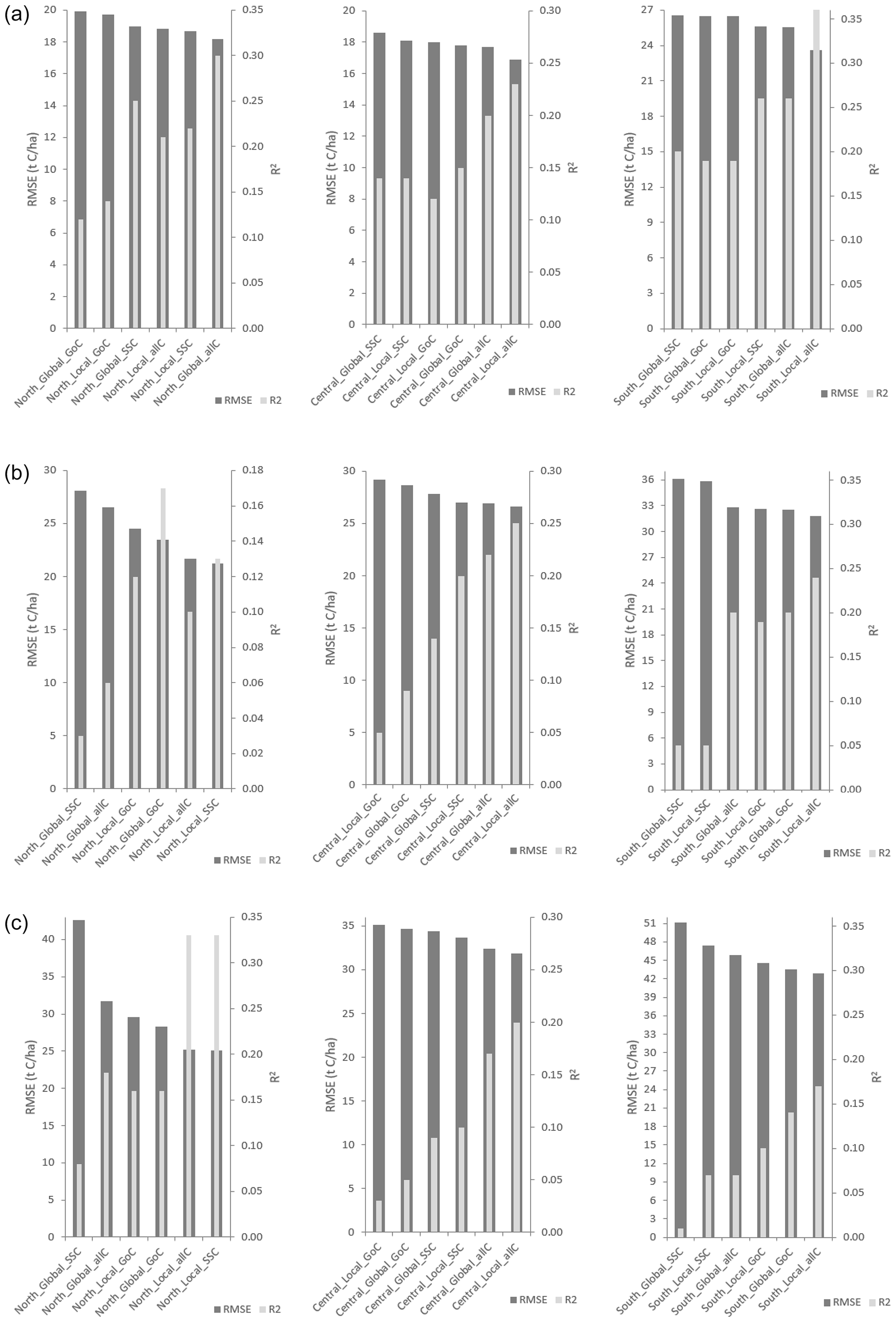
Figure 2Local and global models ranked by decreasing RMSE per sub-area and category of variables along with corresponding R2 (a – litter layer; b – mineral soil layer; c – total soil layer; SSCs – site-specific covariates; GoCs – group of covariates; allCs – all covariates).
The local and global models showed similar trend for the density distribution of actual versus predicted SOC stock (Fig. 3). For Figs. 3 and 4, only global and local models with the lowest RMSE were reported to avoid redundancies. All RF models presented an underestimation of lower and higher values of SOC stock, while an overestimation was observed for the values centred around the means. However, underestimation of high values was less pronounced with the global models over the entire Sweden and also with the predictions for the humus layer. The local model associated with the group of covariates of the mineral soil SOC stock in northern Sweden also presented a pronounced overestimation of the lower values.
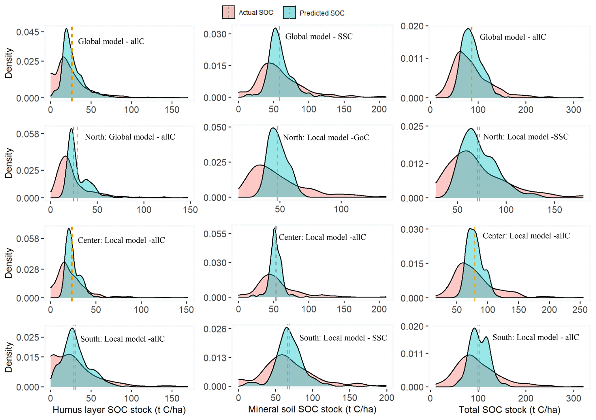
Figure 3Density plots of the actual versus predicted humus layer, mineral soil, and total SOC stock from the local and global random forest models (with lowest root mean square errors). Line – average values; SSCs – site-specific covariates; GoCs – group of covariates; allCs – all covariates; dashed lines – mean of SOC stock.
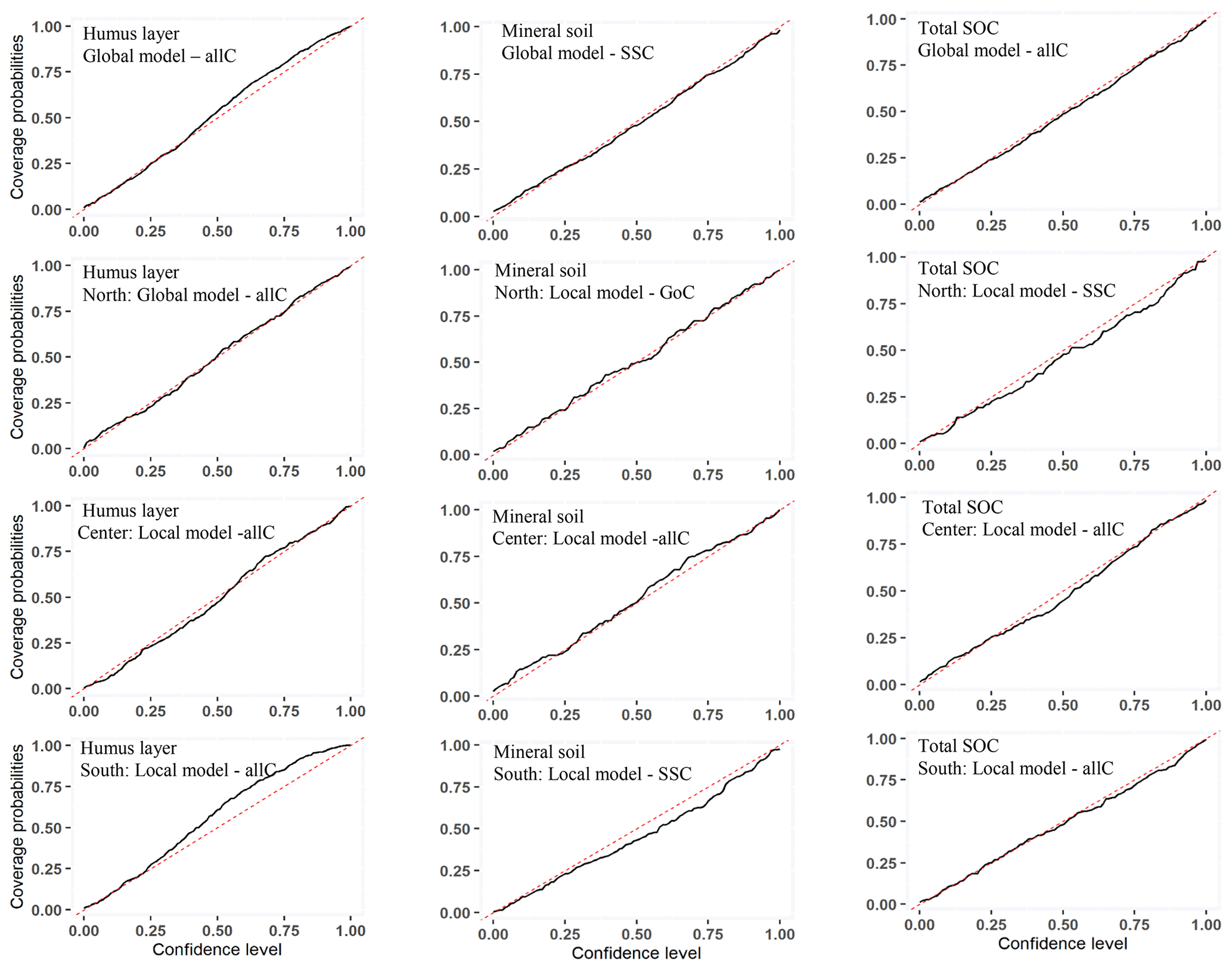
Figure 4Prediction interval coverage probability of the local and global random models for the humus layer, mineral soil, and total SOC stock. SSCs – site-specific covariates; GoCs – group of covariates; allCs – all covariates.
The PICP estimates seem to correspond quite well with the respective confidence level (Fig. 4), except for the humus and mineral SOC stock of southern Sweden. For southern Sweden, it appears that at a higher level of confidence the corresponding PICP is higher for the humus layer and lower for the mineral SOC stock. Considering a 90 % prediction interval, most of the validation observations (80 %–95 %) were located within the prediction interval, especially for models based on specific site covariates or all covariates (Figs. S1a, b, and c in the Supplement).
3.3 Variable importance
The global RF models using only site factors show that (Table 5) the latitude (northing) was the most important variable influencing the distribution the humus layer and the total SOC stock, though it ranked second for the mineral soil. A consistent negative but significant correlation was observed between the different SOC stocks and the latitude, suggesting lower stock northwards no matter the depth.
Table 5Random forest variable importance for the global and local models for the humus layer, mineral soil, and total SOC stock with their associated Pearson's coefficient of correlation with the covariates (values in parenthesis are as follows: * p≤0.05; p≤0.01; p≤0.001).
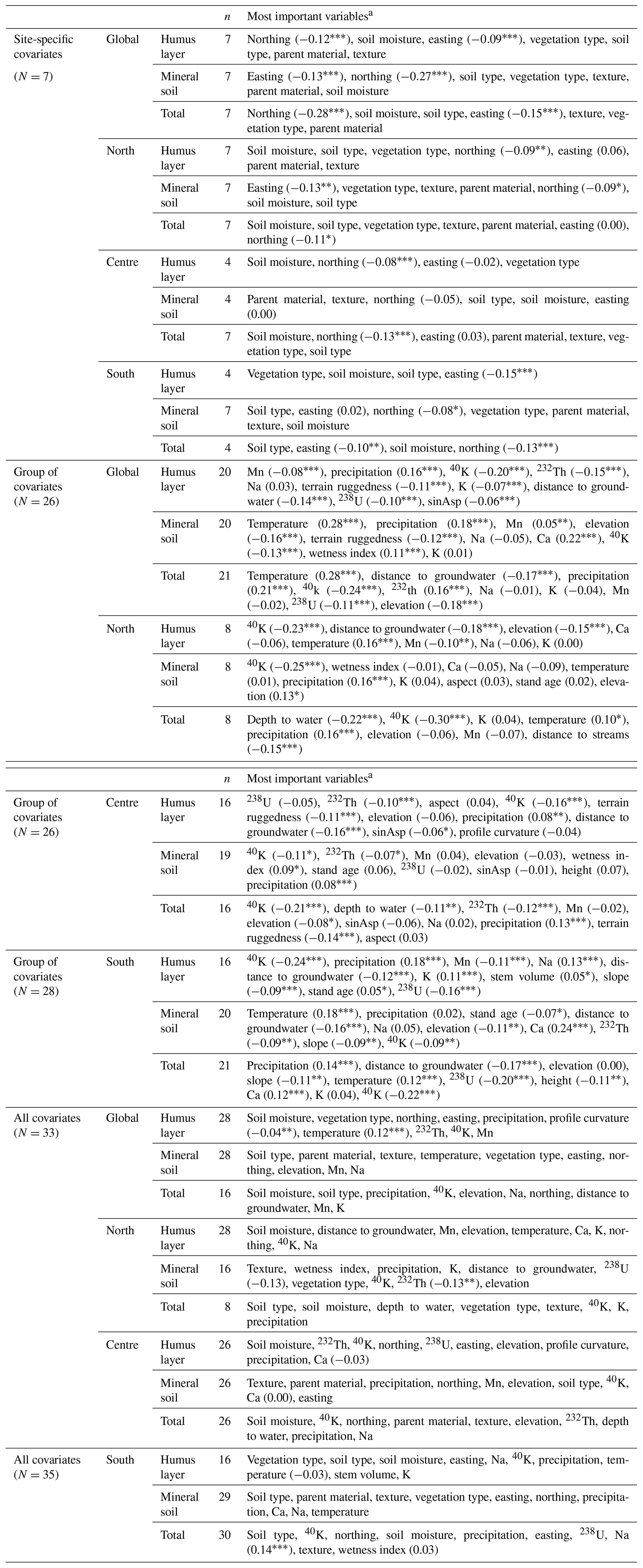
a Site-specific covariates have no correlation values since they are categorical covariates. Pearson's correlation coefficient is provided at the first occurrence for a specific category of covariates and SOC type. N – total number of covariates; n –number of covariates after feature selection.
The site-specific covariates took pre-eminence over the GoCs both at global and local scales when considering models using all covariates (Table 5). The occurrences of soil moisture or soil type among the top two most influential covariates are higher compared to the remaining covariates. For the humus layer SOC stock, the key covariate involved in the prediction was the soil moisture reported both for global and local models, except in southern Sweden where it came as the third key variable. The most prominent covariate in predicting the mineral soil SOC stock with the global allC model was the soil type as also recorded for southern Sweden, while the remaining local models indicated texture for northern and central Sweden. The global model revealed soil moisture and soil type as being the main covariates affecting the prediction of the total SOC stock over Sweden. A similar trend is observed in northern Sweden, while the remaining models recorded 40K as second key variable in addition to soil moisture and soil type for the central and southern Sweden, respectively.
The cumulative contribution of each category of covariates to model accuracy, based on their contribution to the MDA using all covariates, is presented in Fig. 5. Topography covariates greatly influence model accuracy in the northern part of Sweden, contributing to about 30 %–40 % of the model MDA, especially for the humus layer and mineral soil SOC stock. This is further corroborated by a high correlation of these covariates with the SOC stock in northern Sweden (Table 5). For the humus and mineral SOC stock, the importance of topography decreased from the north to the south of Sweden with the gamma ray, site-specific, and climate covariates gaining more prominence (contributing together up to 60 % of MDA) in central Sweden, while site factors were the most influential variable with a share of 40 % of MDA in southern Sweden (Fig. 5). These categories of covariates, which ranked first in central and southern Sweden, were also classified among the top three covariates – site-specific covariates, climate, and gamma ray data – for the global humus layer model.
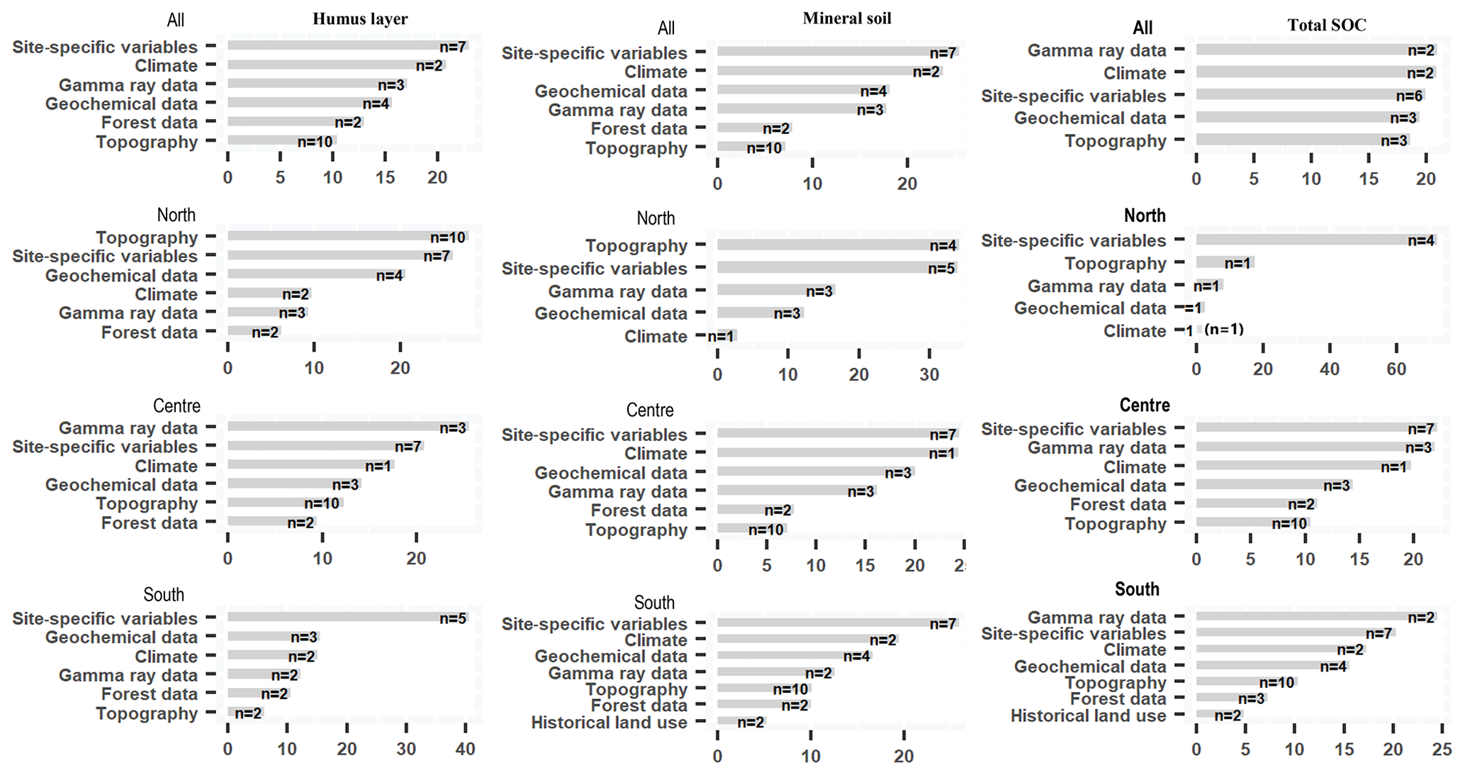
Figure 5Variable importance of the main category of covariates for local and global random models for the humus layer, mineral soil, and total SOC stock.
As observed for the humus layer, topography was less prominent for central and southern Sweden for both mineral soil and total SOC stock (Fig. 5). Site-specific covariates, climate, and geochemical data, which provided the highest contribution to MDA mineral soil for the global model over Sweden, were also the most influential over central and southern Sweden, contributing together up to 60 % and 70 % to the MDA. Gamma ray data seemed to play a key role in the distribution of the total SOC stock, especially in southern Sweden, together with the site-specific covariates and climate. It is important to note that, for the global model of the total SOC layer, the different category of covariates contributed almost equally to the MDA, with the gamma ray and climate taking pre-eminence over the site-specific covariates. The forest covariates had very low contributions as compared to the remaining (Fig. 5) category of covariates, and they were mostly absent from the top 10 (Table 5), while those ranked have very low correlation with the different SOC stock.
3.4 Maps of SOC stock
Figure 6 shows the SOC stock maps from the GoC global and local models. Though the global GoC models generally outperformed the local GoC models (Table 4), their predictive maps generally follow the same pattern. Broadly, there is an increasing gradient of SOC stock from north to south for the humus layer, mineral soil, and total SOC stock. The local models tend to present lower values of SOC stock in northern and central Sweden for the humus layer, while the global model displays higher values over the whole country. For the mineral soil, there seems to be no distinct difference in the spatial prediction of SOC stock, which resulted in a similar pattern from the north to the south for both local and global model maps. Since the total SOC stock is the sum between the humus layer and mineral SOC stock, its spatial distribution follows the same trend, with the lowest SOC recorded in northern and central Sweden while higher stock are located in the south. No matter the type of SOC stock, the coefficient of variation is high and generally above 60 % throughout Sweden.
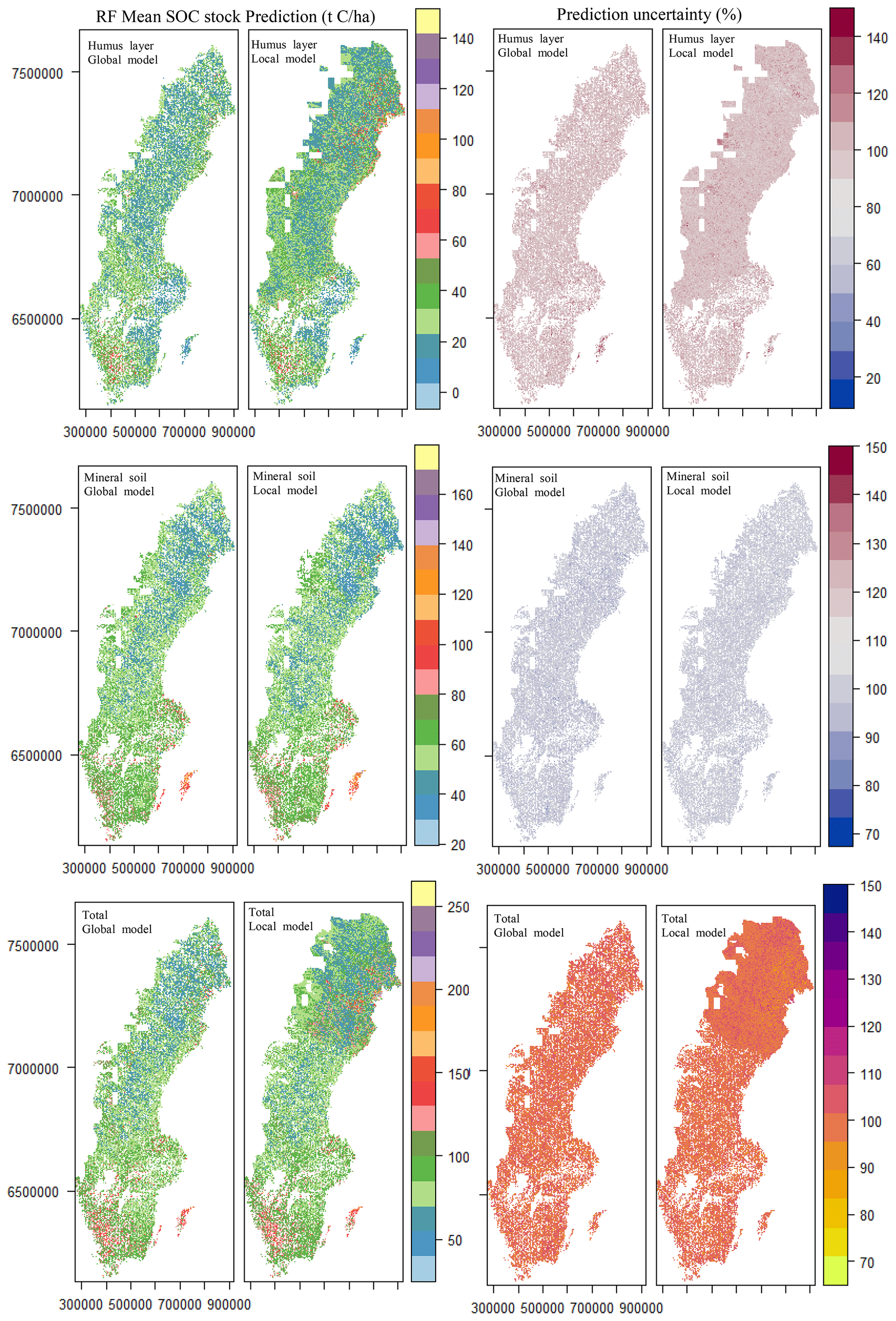
Figure 6Mean SOC stock prediction and prediction uncertainties of the spatial distribution of the humus layer, mineral soil, and total SOC stock based on the group of covariates.
4.1 Prediction with global and local models
This study examined how global and local models differ in predicting the humus layer, mineral soil, and total SOC stock in Swedish forests. The local models recorded lower RMSE at the modelling stage with the cross-validation compared to the global models, except for the southern area. When predictions were carried out on the same validation set, local models, including those of southern Sweden, generally outperformed the global models. This suggests, on the one hand, that global models with higher sample size might not necessarily result in a more accurate model compared to models built from a reduced data set corresponding to a sub-area of a bigger region. On the other hand, the particular case for southern Sweden suggests that, though a global model might present a comparative advantage at modelling stage, it might not necessarily have a better predictive power when confronted with a new set of samples. The findings of this study are in line with those of Somarathna et al. (2016), who also found locally calibrated models to perform better than global models for predicting SOC content. However, the results of the present study differed from the latter in that the comparative advantage was dependent of the category of covariates used.
Findings (Fig. 2) showed that local models which outperformed global models were either associated with all covariates or site-specific covariates. For example, local models in central Sweden required all covariates to outperform global models for the humus layer, mineral soil, and total SOC stock. The same pattern was observed for southern Sweden, except for the mineral SOC stock for which the best local model was associated with the SSCs. The local best model for the total SOC stock in northern Sweden was also associated with SSCs. The higher occurrences of SSCs and allCs with the best local models showed that modelling with GoCs alone is not the optimal choice. On the one hand, forest SSCs are more relevant for capturing the local variability in the sampling plots than the other covariates which are mostly remote sensing products. When both SSCs and GoCs are used as covariates, the locally specific information at plot scale are complemented by higher-scale covariates which cover a larger range of the feature space, resulting in model improvement, especially for the humus layer.
In addition, using both site characteristics and remotely sensed products for predicting SOC stock generally increased the variance explained with both cross-validation and independent validation methods for the humus layer, mineral soil, and total SOC stock. However, despite the combination of these two categories of covariates, the accuracy of the SOC stock prediction remained low for both the global models (maximum R2 is 0.30) and local models (maximum R2 is 0.33). There seems to be no study comparable in scope and methodology targeting the prediction of SOC stock in forest soils. The closest is the digital mapping of SOC stock for the humus layer and mineral stock using machine learning models such as RF and the k nearest neighbour (kNN) based on data set from the national forest inventory of the USA (Cao et al., 2019). The authors also found a lower fit between predicted and observed SOC stock after the independent validation and reported an R2 of 0.20 and 0.11 for the humus layer, while recording an R2 of 0.33 and 0.28 for the mineral soil, respectively, for the RF and kNN models. Other studies conducted in temperate forests for predicting SOC stock also showed poor goodness of fit values, with a cross-validation R2 of 0.22 (1 m depth) with the boosted regression trees (Ottoy et al., 2017). For other soil properties, Mansuy et al. (2014) reported, for some Canadian managed forest, an R2 of 0.04 and 0.05 for SOC content in the humus layer and mineral soil, respectively, with the kNN, while Beguin et al. (2017) recorded, for the Canadian forest, an R2 of 0.05 for SOC content for the mineral soil with RF model.
Low explained variances in predictive modelling could be related to different factors (Nelson et al., 2011). For example, the omission of key covariates with greater explanatory power or conversely using non-essential covariates with very low explanatory power which only increase the prediction error variance. Omitting key covariates in relation to SOC stock for forest ecosystem in the present study is less likely since covariates considered in this study well represent the surrogates for soil forming factors considered in the Soils, Climate, Organisms, Parent material, Age and (N) space or spatial position (SCORPAN) equation defined by McBratney et al. (2003). In addition, the removal of redundant and non-informative covariates was carried out via dimension reduction, with the exclusion of highly correlated covariates and elimination of some others via recursive feature elimination. However, the Pearson correlations (min = 0; max = 0.28) between covariates and the different SOC stock were found to be poor though significant for most of the predictors (Table 5; Figs. S2–S4). This could be expected because the data cover a wide range of different site conditions, soil types, and parent materials.
Another source of the errors could be inherent to the model, with prediction accuracy varying with different type of model. Many studies have already compared different machine learning models and concluded that RF generally has a strong predictive ability in different ecosystems (Cao et al., 2019; Forkuor et al., 2017; Wang et al., 2018). Preliminary steps in the present study also tested extreme gradient boosting and Cubist models (results not shown) alongside the RF, with the latter displaying higher predictive capabilities. On the other hand, applying geostatistical approaches (Fig. S5) for the humus layer, mineral soil, and total SOC stock revealed very low spatial autocorrelation for the different SOC stock, suggesting that the structure of the SOC data has a shorter range than the sampling interval. For soil properties which vary over short distance, such as SOC stock, data-driven models such as RF might capture the inherent variability better when modelling data are a good representative of the phenomenon that the SOC stock is subject to in the landscape, including small-scale variation. Beguin et al. (2017) recorded poor performance of different models, including RF, for predicting C : N because the sampling scheme failed to capture the distance variation (< 20 km) at which a better accuracy would have occurred. Model accuracy would likely improve if more samples covering the spatial variability in each inventory plot were taken. The increase in RMSE with depth recorded for some models is consistent with previous studies, where the prediction of lower soil layers resulted in lower accuracy (Henderson et al., 2005; Yam et al., 2019). This may be due to a higher sensitivity of the humus layer which is directly exposed to the influence of environmental covariates.
The estimates of SOC stocks are slightly biased towards the extreme values, with an underestimation of the lowest and highest values for both local and global models (Fig. 3). This tends to confirm earlier findings which reported issues related to the underestimation or overestimation of extreme values by the RF model (Čeh et al., 2018; Hu et al., 2020; Horning, 2010). On the one hand, this seems to be typical for regression models with RF because predictions are the average values of all of the trees, with a tendency to predict the mean when the correlation of response and covariate is weak. On the other hand, this may also be related to an under-representation of the lower and higher values compared to those centred around the mean in the training data set. However, though underestimation of the lowest and highest values could be recorded for all models, the 90 % PICP shows, in general, that the 90 % prediction interval adequately covers the observed values of the humus, mineral, and total SOC stock layers (Fig. 4). This is an indication that the prediction intervals are accurate representative of the prediction uncertainties for each of these SOC stocks for both local and global models. However, for southern Sweden, the PICP presented higher values for the humus layer and lower values for the mineral SOC stock with increasing level of confidence, suggesting a higher level of uncertainties in the predictions. This could be attributed to southern Sweden being characterized by a longer management history and more intensive forestry compared to northern Sweden (Angelstam and Pettersson, 1997), leading to a diversity in forest management patterns with potential feedback on SOC stock distribution.
4.2 Variable importance and modelling accuracy
SOC stocks in forest soils are the product of the dynamic equilibrium between the input flux of plant-derived materials and output flux of carbon as a result of decomposition. Classical soil-forming factors – climate, organisms (vegetation, fauna, and human activities), topography, parent material, and time – are known to govern the amount and distribution of SOC stock. Though covariates used as proxy for these soil-forming factors were considered separately for the sake of analysis in this study, they are actually involved in dynamic interactions leading to complex soil processes in the landscape.
With the global RF models using only site-specific covariates, the latitude (northing) was the main variable driving the distribution of the SOC stock, with a negative correlation suggesting lower stock to the north (Table 5). The latitudinal gradient (Millberg et al., 2015) in Sweden also results in climatic gradient (Jungqvist et al., 2014), which, in turn, interacts with topography (Johansson and Chen, 2003) to determine the heterogeneity in net primary production in relation to the spatial variability in precipitation and temperature. Even at a regional level, the latitude was still critical and was mostly present among the top 10 covariates being selected by the local RF models using all covariates (Table 5). However, climate and topographical covariates were consistently overshadowed by SSCs when all the covariates were used for modelling both at a national and regional scale. Though precipitation regulates net primary productivity (NPP) and temperature controls microbial decomposition of organic matter, their local variability is generally small (Wiesmeier et al., 2019). This makes them less relevant in contrast to SSCs taken at plot level, which describe more closely the factors controlling the decomposition and stabilization of organic matter.
Among the site characteristics, the soil moisture was the key site factor affecting the humus layer SOC stock, especially in the northern and central Sweden, while vegetation type was ranked first in southern part of Sweden (Table 5). The box plots of these two covariates showed that they clearly have different distributions of SOC stock in the humus layer, although some of the interquartile ranges overlap (Fig. S6). As observed for the humus layer, soil moisture was the most important variable associated with total SOC stock along with the soil type. For a sequence from dry to moist soils, there was an increase in SOC stock in the humus layer and for the mineral and total stock (box plot of soil moisture in Figs. S6–S8). This might be explained by higher productivity in litter supply as water is more available in the tree root zone of fresh and moist sites. On the other hand, these latter soils are subject to a longer period of saturation (reducing conditions) that slows down decomposition. The impact of soil moisture could also be noted when considering the partial dependence plot of the RF global model of the humus layer showing the interaction between the soil moisture class and vegetation type (Fig. S9a). Each vegetation type consistently tends towards higher values of SOC stock for moist sites compared to dry and fresh sites.
Generally, soil type and texture were ranked by the allC global models as being the top covariates influencing the SOC stock in the mineral soil (Table 5). The link between these two covariates could be related to the soil moisture content of their classes. On the one hand, soil types (Histosols and Gleysols) with fine texture (fine silt and clay) and high moisture content are more subject to reducing conditions with higher SOC stock compared to soils (Leptosols and Arenosols) with a coarse (stone, boulder, and coarse sand) texture. On the other hand, the relevance of soil texture as a predictor of SOC could be related to the physicochemical SOC stabilization mechanisms. Clay minerals and clay- and silt-sized particles generally have a positive correlation with mineral SOC stocks, as the association of organic matter with mineral surfaces and occlusion inside aggregates hinders microbial decomposition and enhances SOC accumulation (Lützow et al., 2006; Zhang et al., 2020).
The addition of the other group of covariates (GoCs) to the site-specific covariates resulted in limited improvement for both global and local models (Tables 3–4). This suggests that their level of distinct complementarity in the feature space is low as the GoCs might be carrying redundant information with the site-specific covariates in relation to the humus layer, mineral soil, and total stock. For example, the prominence of site-specific covariates over topographical covariates (Table 5; allCs) might be due to the fact they are indirectly incorporated into the definition of the site-specific covariates. For this study, wetness index, distance to groundwater, and depth to water are indexes used to characterize soil moisture, while gamma ray data describe parent material. A similar observation was shared by Wiesmeier et al. (2011) who, also recorded land use and soil type as being key covariates affecting SOC stock, while topographic covariates contributed very weakly to model accuracy using random forest. However, though ranked low among all covariates (Table 5; allCs), the cumulated variable importance analysis showed that topographical covariates stood out in contributing to model accuracy in northern Sweden (Fig. 5) but were less relevant in the south. Obviously, higher elevation and derivatives in northern Sweden explain such an influence on the SOC stock.
Next to site characteristics and climate, the cumulative gamma ray data were more consistent in contributing to model accuracy of the total SOC stock compared to geochemical data, with the individual ranking further revealing a higher occurrence of radioactive K both at the global and regional level (Table 5; Fig. 5). This suggests that K-bearing minerals of the parent material have greater explanatory power over total SOC stock than U and Th, the nature of which might require further studies. Malone et al. (2009) also recorded gamma K as being the key covariate for mapping SOC stock in an agriculture dominated land use in Australia.
The geochemical data were revealed to be the key covariates in the distribution of SOC stock in southern Sweden, especially for the humus layer (Na) and mineral stock (Ca and Na), though of a much lower magnitude compared to site-specific covariates. However, base cations seemed not to primarily affect SOC distribution but rather environmental covariates that regulate their dynamics. The low ranking of forest parameters may be related to (1) their low correlations with the SOC stock data and (2) the fact that the data set cut across different data forest types without any specific stratification, which could have created a homogeneous strata for modelling. However, the focus of the present study was not on a specific forest type, which could have further reduced the training data set, while machine learning models require high data samples to learn patterns and accurately predict target values on independent data sets.
4.3 Spatial prediction of SOC stock
The maps of the humus layer, mineral soil, and total stock present a pattern of the increasing accumulation of SOC stocks from south to north, with the highest uncertainties in the southern part of Sweden regardless of the predicting models (Fig. 6). In general, it is expected that the global latitudinal trend will result in increasing stocks in higher latitudes, which correspond to colder and humid regions. Possible explanations are associated with slower microbial decomposition rates, while other studies suggest non-conducive soil conditions such as water logging, low pH values, and high aluminium concentration as being the main constraints (Dieleman et al., 2013; Hobbie et al., 2000; Wiesmeier et al., 2019).
The contrary configuration observed in the maps, with a decreasing south–north distribution in the SOC stock for the humus layer and mineral soil (Fig. S10), is consistent with findings from different studies (Kleja et al., 2008; Fröberg et al., 2011; Hyvonen et al., 2008). These studies advocate that the high SOC stocks in the south could be related to a higher deposition of nitrogen (N) compared to central and northern Sweden. It has been suggested that N deposition results in both increasing litter inputs and increasing mean residence time. Also, high concentrations of inorganic N inhibit the activities of lignin-degrading phenol oxidase released by microorganisms (Zak, 2017; Carreiro et al., 2000). However, a warmer climate makes trees grow faster, along with a higher litter input, in the south than in the north. With the co-occurring north–south gradient of temperature (lower), pH (higher), soil carbon (lower; Iwald, 2016; Framstad, 2013), and N deposition might have contributed to the strengthening of the north–south SOC stock gradient. As southern Sweden (Fig. 6) recorded a higher range in SOC stocks, the associated average variation around the mean was also larger.
4.4 Implication and limitations of the study
The present study compared a local and a global modelling approach for DSM. To the question of which approach to use when mapping a big area, our research showed that it is dependent on the type of covariates available. In general, building local models for sub-areas of the study region will require having covariates which correlate most with the sampling sites, thereby offering a better description at a smaller scale. In this study, the site characteristics were better representative of the sampling locations, and their local models generally performed better than global models. In situations where such site characteristics data are not available, it would be preferable to use a global model for the whole area. However, machine learning models such as RF are data driven, and therefore, results will vary according to the specificity of a given area. Therefore, there is no silver bullet to use in the approach for any specific area, and it will be necessary to draw conclusions from the modelling results. However, it is very likely that the combination of site characteristic with the GoC data would result in higher accuracy at both a local and global scale than using only the group of covariates dominated by remote sensing data.
Table 6Independent validation of the global and local random forest models based on the mapped site-specific covariates compared to models based on observed site-specific covariates and grouped of covariates.
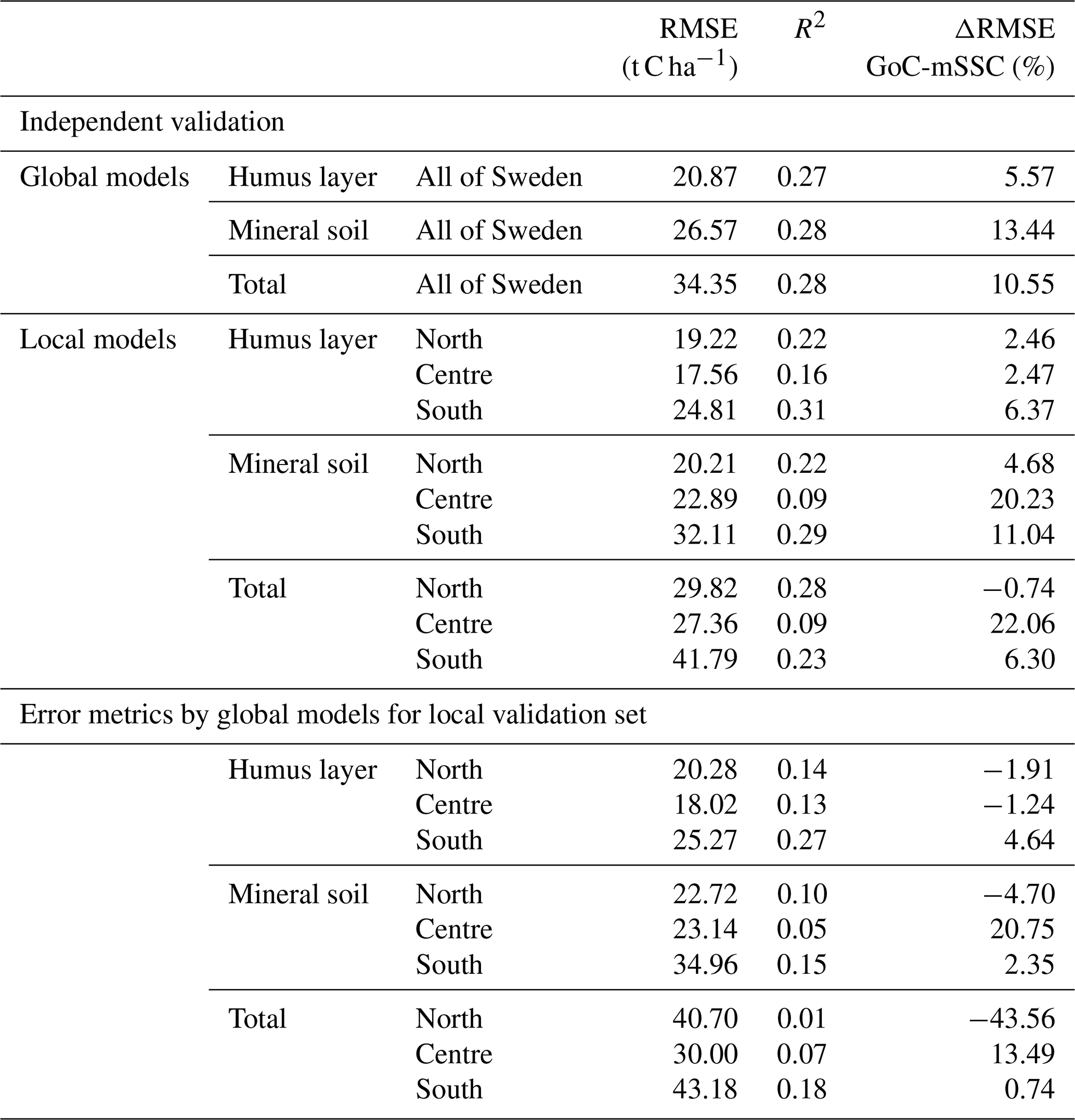
ΔRMSE GoC-mSSC (%) – percentage estimate of the difference between the root mean square error of models based on group of covariates and mapped site-specific covariates; negative values – models with mapped site-specific covariates present a higher root mean square error compared to models based either on observed, site-specific variables or a group of covariates; positive values – models with mapped site-specific covariates present a lower root mean square error compared to models based on either observed, site-specific variables or a group of covariates; R2 – coefficient of determination.
The maps produced with the GoC global and local models for the humus layer, mineral soil, and total SOC stock accurately present the distribution of SOC stocks observed for Sweden in many studies. Given that the underlying models were not the most accurate in the present study, such maps should be treated with caution, especially with the associated high coefficient of variation. However, they could serve as a high-resolution indicator of the spatial trend in SOC stocks at different depths for the landscape of the Swedish forest. In addition, the use of a DSM approach in the present study allows flexibility in future improvements upon the acquisition of new covariates or data points, repeatability in modelling with the application of the same modelling principles using open-source software (e.g. R), and the ability to capitalize on multi-source information (topography, site characteristics, forest data, gamma radiometry, and geochemical data). Therefore, smaller counties could evaluate this approach against their own data sets for mapping other soil properties (pH, texture, Fe, Al, etc.) and SOC stocks for local applications.
DSM relies on existing maps for building regression models and for mapping. The quality and accuracy of the predictions depend, as discussed earlier, on choosing the most relevant covariates in relation to the target to be predicted. The present study revealed that covariates which were available as maps did contribute to the MDA, but site characteristics were more prominent in relation to the SOC stocks in Sweden. This might suggest that mapping these variables that were more decisive for SOC stock prediction and including them as covariates for mapping may improve accuracy. Since the primary focus of the present study was mainly to evaluate the GoC data versus the SSC data at different scales of modelling, and not primarily for making a map, the observed data of the latter were used. However, since only the observed data of the site characteristics were considered, this study fails to consider that the mapping of these site characteristics would involve modelling errors, and the propagation of these errors into the final maps of these site variables might actually reduce their predictive power. For completeness, we carried out a preliminary mapping of the site characteristics (Fig. S11) using additional soil inventory data, random forest, and the GoCs as predictors. These mapped site characteristics (mSSCs) were then used as covariate for predicting the SOC stocks.
Table 6 presents the error metrics after independent validation for both local and global models, along with the percentage margin of the RMSE in relation to the models based on GoCs. First, the local mSSC-based models still recorded a lower RMSE compared to global mSSC models. Compared to the GoC models, the overall positive percentage margin of the RMSE for the independent validations indicated that the mSSC models recorded the lowest RMSE. However, when assessing the RMSE margin between the global models of GoCs and SSCs, negative percentages were mainly recorded for northern Sweden, independently of the depth. This indicated that the mSSC-based global models were less accurate at predicting SOC stocks locally in northern Sweden. On the other hand, the mSSC-based local model did present a better prediction for northern Sweden for the humus layer and mineral SOC stock. The mean SOC predictions based on the mSSCs showed a stronger increasing gradient from northern to southern Sweden (Fig. S12) compared to the pattern observed with the GoC maps. However, the uncertainty distribution was of a similar magnitude (Fig. S12) to those observed for the maps based on GoCs, probably due to error propagations, as these covariates were used to make the site-specific characteristics maps. This suggests that the SSCs should still be supplemented for improvement at this stage with other covariates different from the GoCs, such as multi-temporal spectral (e.g. normalized difference vegetation index) data that are able to capture vegetation dynamic in forests. Notwithstanding the possibility of error propagation, the study of which was beyond the scope our focus, the preceding results tend to confirm the potential of the high-resolution maps of the site characteristics to contribute to the improvement of SOC stock prediction as compared to using only the GoC data. Given that the preliminary mappings of the SSCs recorded low kappa (0.17–0.48) values (Fig. S11) at this stage, further improvements are still necessary to improve their SOC stock predictive ability and the associated coefficient of variations.
This study has shown that:
-
Local models have a comparative advantage over global models when using either site characteristics alone or the combination of the latter with a group of covariates dominated by remotely sensed data.
-
Using a group of covariates dominated by remote sensing data with a soil inventory data set indicates that such covariates have limited predictive ability compared to site-specific covariates.
-
The most important covariates that influence the humus layer, mineral soil, and total SOC stock were related to the site-characteristic covariates consisting of the soil moisture class, vegetation type, soil type, and soil texture.
All code has been made available in an R file (.pdf) in the Supplement (Asset S1).
The data used in this study are available upon reasonable request to Johan Stendahl (johan.stendahl@slu.se). The high-resolution digital elevation models (DEM) should be requested by contacting the Swedish national mapping agency (Lantmäteriet; https://www.lantmateriet.se, last access: 1 April 2019). The climate data used (MAT and MAP) can be downloaded from WorldClim (https://www.worldclim.org/, Fick and Hijmans, 2017). The geochemical and gamma ray data can be obtained from the Geological Survey of Sweden (SGU; https://www.sgu.se, last access: 25 March 2019). Requests for forest maps should be directed to the Swedish Forest Agency (Skogsstyrelsen; https://www.skogsstyrelsen.se, last access: 15 January 2019). The data set related to the historical map series can be freely downloaded from the Figshare repository at https://doi.org/10.17045/sthlmuni.4649854 (Auffret et al., 2017b).
The supplement related to this article is available online at: https://doi.org/10.5194/soil-7-377-2021-supplement.
The conceptualization of the study for this paper was done by KOLH, with input from JS, ML, and EK. The data curation and formal analysis, methodology, and visualization for the paper was performed by KOLH, with substantial input from JS, ML, and EK. KOLH wrote the initial draft, and all authors were involved in the reviewing and editing of the paper.
The authors declare that they have no conflict of interest.
Publisher's note: Copernicus Publications remains neutral with regard to jurisdictional claims in published maps and institutional affiliations.
We thank all the reviewers and the editor for their valuable comments on the paper.
This work has been supported by the Swedish Research Council Formas.
This paper was edited by Nicolas P. A. Saby and reviewed by Madlene Nussbaum and two anonymous referees.
Andersson, M., Carlsson, M., Ladenberger, A., Morris, G., Sadeghi, M., and Uhlbäck, J.: Geokemisk Atlas Över Sverige-Geochemical Atlas of Sweden, Sveriges Geologiska Undersökning, Uppsala, Sweden, 2014.
Angelstam, P. and Pettersson, B.: Principles of present Swedish forest biodiversity management, Ecol. Bull., 46, 191–203, 1997.
Auffret, A. G., Kimberley, A., Plue, J., Skånes, H., Jakobsson, S., Waldén, E., Wennbom, M., Wood, H., Bullock, J. M., Cousins, S. A., and Gartz, M.: HistMapR: Rapid digitization of historical land-use maps in R, Methods Ecol. Evol., 8, 1453–1457, 2017. Auffret, A. G., Kimberley, A., Plue, J., Skånes, H., Jakobsson, S., Waldén, E., Wennbom, M., Wood, H., Bullock, J. M., Cousins, S. A. O., Gartz, M., Hooftman, D. A. P., and Tränk, L.: Data from: HistMapR: Rapid digitization of historical land-use maps in R, Stockholm University [data set], https://doi.org/10.17045/sthlmuni.4649854.v2, 2017b.
Beguin, J., Fuglstad, G.-A., Mansuy, N., and Paré, D.: Predicting soil properties in the Canadian boreal forest with limited data: Comparison of spatial and non-spatial statistical approaches, Geoderma, 306, 195–205, 2017.
Breiman, L.: Random Forests, Mach. Learn., 45, 5–32, https://doi.org/10.1023/A:1010933404324, 2001.
Buchholz, T., Friedland, A. J., Hornig, C. E., Keeton, W. S., Zanchi, G., and Nunery, J.: Mineral soil carbon fluxes in forests and implications for carbon balance assessments, GCB Bioenergy, 6, 305–311, 2014.
Cao, B., Domke, G. M., Russell, M. B., and Walters, B. F.: Spatial modeling of litter and soil carbon stocks on forest land in the conterminous United States, Sci. Total Environ., 654, 94–106, 2019.
Carreiro, M. M., Sinsabaugh, R. L., Repert, D. A., and Parkhurst, D. F.: Microbial enzyme shifts explain litter decay responses to simulated nitrogen deposition, Ecology, 81, 2359–2365, 2000.
Čeh, M., Kilibarda, M., Lisec, A., and Bajat, B.: Estimating the performance of random forest versus multiple regression for predicting prices of the apartments, SPRS Int. J. Geo-Inf., 7, 168, https://doi.org/10.3390/ijgi7050168, 2018.
Conrad, O., Bechtel, B., Bock, M., Dietrich, H., Fischer, E., Gerlitz, L., Wehberg, J., Wichmann, V., and Böhner, J.: System for Automated Geoscientific Analyses (SAGA) v. 2.1.4, Geosci. Model Dev., 8, 1991–2007, https://doi.org/10.5194/gmd-8-1991-2015, 2015.
Dieleman, W. I. J., Venter, M., Ramachandra, A., Krockenberger, A. K., and Bird, M. I.: Soil carbon stocks vary predictably with altitude in tropical forests: implications for soil carbon storage, Geoderma, 204, 59–67, 2013.
Dowling, T. P., Alexanderson, H., and Möller, P.: The new high-resolution LiDAR digital height model (“Ny Nationell Höjdmodell”) and its application to Swedish Quaternary geomorphology, GFF, 135, 145–151, 2013.
Erdi-Krausz, G., Matolin, M., Minty, B., Nicolet, J. P., Reford, W. S., and Schetselaar, E. M.: Guidelines for radioelement mapping using gamma ray spectrometry data: also as open access e-book, International Atomic Energy Agency (IAEA), Austria, 2003.
Fick, S. E. and Hijmans, R. J.: WorldClim 2: new 1-km spatial resolution climate surfaces for global land areas, Int. J. Climatol., 37, 4302–4315, https://doi.org/10.1002/joc.5086, 2017 (data available at: https://www.worldclim.org/, latest access: 20 June 2019).
Forkuor, G., Hounkpatin, O. K. L., Welp, G., and Thiel, M.: High Resolution Mapping of Soil Properties Using Remote Sensing Variables in South-Western Burkina Faso: A Comparison of Machine Learning and Multiple Linear Regression Models, PLoS ONE, 12, e0170478, https://doi.org/10.1371/journal.pone.0170478, 2017.
Framstad, E.: Biodiversity, carbon storage and dynamics of old northern forests, Nordic Council of Ministers, Copenhagen, 2013.
Fröberg, M., Tipping, E., Stendahl, J., Clarke, N., and Bryant, C.: Mean residence time of O horizon carbon along a climatic gradient in Scandinavia estimated by 14C measurements of archived soils, Biogeochemistry, 104, 227–236, 2011.
Gomes, L. C., Faria, R. M., de Souza, E., Veloso, G. V., Schaefer, C. E. G., and Fernandes Filho, E. I. J. G.: Modelling and mapping soil organic carbon stocks in Brazil, Geoderma, 340, 337–350, 2019.
Grimm, R., Behrens, T., Marker, M., and Elsenbeer, H.: Soil organic carbon concentrations and stocks on Barro Colorado Island – Digital soil mapping using Random Forests analysis, Geoderma, 146, 102–113, https://doi.org/10.1016/j.geoderma.2008.05.008, 2008.
Hastie, T., Tibshirani, R. J., and Friedman, J. H.: The elements of statistical learning: data mining, inference, and prediction, Springer, New York, 2011.
Henderson, B. L., Bui, E. N., Moran, C. J., and Simon, D. A. P.: Australia-wide predictions of soil properties using decision trees, Geoderma, 124, 383–398, 2005.
Hobbie, S. E., Schimel, J. P., Trumbore, S. E., and Randerson, J. R.: Controls over carbon storage and turnover in high-latitude soils, Glob. Change Biol., 6, 196–210, 2000.
Horning, N.: Random Forests: An algorithm for image classification and generation of continuous fields data sets, in: Proceedings of the International Conference on Geoinformatics for Spatial Infrastructure Development in Earth and Allied Sciences, 911, Osaka, Japan, 2010.
Hounkpatin, O. K., de Hipt, F. O., Bossa, A. Y., Welp, G., and Amelung, W. J. C.: Soil organic carbon stocks and their determining factors in the Dano catchment (Southwest Burkina Faso), Catena, 166, 298–309, 2018.
Hu, Y., Xu, X., Wu, F., Sun, Z., Xia, H., Meng, Q., Huang, W., Zhou, H., Gao, J., and Li, W.: Estimating Forest Stock Volume in Hunan Province, China, by Integrating In Situ Plot Data, Sentinel-2 Images, and Linear and Machine Learning Regression Models, Remote Sens., 12, 186, https://doi.org/10.3390/rs12010186, 2020.
Hyvonen, R., Persson, T., Andersson, S., Olsson, B., Agren, G. I., and Linder, S.: Impact of long-term nitrogen addition on carbon stocks in trees and soils in northern Europe, Biogeochemistry, 89, 121–137, https://doi.org/10.1007/s10533-007-9121-3, 2008.
Iwald, J.: Acidification of Swedish forest soils, SLU Service/Repro, Uppsala, 2016.
Jandl, R., Lindner, M., Vesterdal, L., Bauwens, B., Baritz, R., Hagedorn, F., Johnson, D. W., Minkkinen, K., and Byrne, K. A.: How strongly can forest management influence soil carbon sequestration?, Geoderma, 137, 253–268, 2007.
Jenny, H.: Factors of Soil Formation A System of Quantitave Pedology, Dover Earth Science, 1941.
Johansson, B. and Chen, D.: The influence of wind and topography on precipitation distribution in Sweden: Statistical analysis and modelling, Int. J. Climatol., 23, 1523–1535, 2003.
Jungqvist, G., Oni, S. K., Teutschbein, C., and Futter, M. N.: Effect of climate change on soil temperature in Swedish boreal forests, PloS one, 9, e93957, https://doi.org/10.1371/journal.pone.0093957, 2014.
Kauppi, P. E., Posch, M., and Pirinen, P.: Large impacts of climatic warming on growth of boreal forests since 1960, PLoS One, 9, e111340, https://doi.org/10.1371/journal.pone.0111340, 2014.
Kleja, D. B., Svensson, M., Majdi, H., Jansson, P.-E., Langvall, O., Bergkvist, B., Johansson, M.-B., Weslien, P., Truusb, L., and Lindroth, A.: Pools and fluxes of carbon in three Norway spruce ecosystems along a climatic gradient in Sweden, Biogeochemistry, 89, 7–25, 2008.
Kuhn, M.: Caret: classification and regression training, Astrophysics Source Code Library, 1, 05003, available at: https://cran.r-project.org/web/packages/caret/index.html (last access: 2 July 2021), 2015.
Kuhn, M.: caret: Classification and regression training [Computer software manual], available at: https://CRAN.R-project.org/package=caret, last access: 10 April 2019.
Kumar, P., Pandey, P. C., Singh, B. K., Katiyar, S., Mandal, V. P., Rani, M., Tomar, V., and Patairiya, S.: Estimation of accumulated soil organic carbon stock in tropical forest using geospatial strategy, Egyptian Journal of Remote Sensing and Space Science, 19, 109–123, 2016.
Lawrence, I. and Lin, K.: A concordance correlation coefficient to evaluate reproducibility, Biometrics, 45, 255–268, 1989.
Lidberg, W., Nilsson, M., and Ågren, A.: Using machine learning to generate high-resolution wet area maps for planning forest management: A study in a boreal forest landscape, Ambio, 49, 1–12, 2019.
Lützow, M. v., Kögel-Knabner, I., Ekschmitt, K., Matzner, E., Guggenberger, G., Marschner, B., and Flessa, H.: Stabilization of organic matter in temperate soils: mechanisms and their relevance under different soil conditions – a review, Eur. J. Soil Sci., 57, 426–445, 2006.
Mallik, S., Bhowmik, T., Mishra, U., and Paul, N.: Mapping and prediction of soil organic carbon by an advanced geostatistical technique using remote sensing and terrain data, Geocarto Int., 1–17, https://doi.org/10.1080/10106049.2020.1815864, online first, 2020.
Malone, B. P., McBratney, A. B., Minasny, B., and Laslett, G. M.: Mapping continuous depth functions of soil carbon storage and available water capacity, Geoderma, 154, 138–152, 2009.
Mansuy, N., Thiffault, E., Paré, D., Bernier, P., Guindon, L., Villemaire, P., Poirier, V., and Beaudoin, A.: Digital mapping of soil properties in Canadian managed forests at 250m of resolution using the k-nearest neighbor method, Geoderma, 235, 59–73, 2014.
McBratney, A. B., Santos, M. M., and Minasny, B.: On digital soil mapping, Geoderma, 117, 3–52, 2003.
Meinshausen, N.: Quantile regression forests, J. Mach. Learn. Res., 7, 983–999, 2006.
Millberg, H., Boberg, J., and Stenlid, J.: Changes in fungal community of Scots pine (Pinus sylvestris) needles along a latitudinal gradient in Sweden, Fungal Ecol., 17, 126–139, 2015.
Minasny, B. and McBratney, A. B.: Digital soil mapping: A brief history and some lessons, Geoderma, 264, 301–311, 2016.
Murphy, P. N. C., Ogilvie, J., Castonguay, M., Zhang, C.-f., Meng, F.-R., and Arp, P. A.: Improving forest operations planning through high-resolution flow-channel and wet-areas mapping, Forest.Chron., 84, 568–574, 2008.
Nelson, M., Bishop, T., Triantafilis, J., and Odeh, I.: An error budget for different sources of error in digital soil mapping, Eur. J. Soil Sci., 62, 417–430, 2011.
Nilsson, M., Nordkvist, K., Jonzén, J., Lindgren, N., Axensten, P., Wallerman, J., Egberth, M., Larsson, S., Nilsson, L., and Eriksson, J.: A nationwide forest attribute map of Sweden predicted using airborne laser scanning data and field data from the National Forest Inventory, Remote Sens. Environ., 194, 447–454, 2017.
Nilsson, T. and Lundin, L.: Prediction of bulk density in Swedish forest soils from the organic carbon content and soil depth, Reports in Forest Ecology & Forest Soils 91, Swedish University of Agricultural Sciences, Uppsala, Sweden, 39 pp., 2006.
Ortiz, C. A., Liski, J., Gärdenäs, A. I., Lehtonen, A., Lundblad, M., Stendahl, J., Ågren, G. I., and Karltun, E. J. E. M.: Soil organic carbon stock changes in Swedish forest soils – a comparison of uncertainties and their sources through a national inventory and two simulation models, Ecol. Modell., 251, 221–231, 2013.
Ottoy, S., De Vos, B., Sindayihebura, A., Hermy, M., and Van Orshoven, J.: Assessing soil organic carbon stocks under current and potential forest cover using digital soil mapping and spatial generalisation, Ecol. Indic., 77, 139–150, 2017.
Pan, Y., Birdsey, R. A., Fang, J., Houghton, R., Kauppi, P. E., Kurz, W. A., Phillips, O. L., Shvidenko, A., Lewis, S. L., and Canadell, J. G.: A large and persistent carbon sink in the world's forests, Science, 333, 1201609, https://doi.org/10.1126/science.1201609, 2011.
Piikki, K., Wetterlind, J., Söderström, M., and Stenberg, B. J. P. a.: Three-dimensional digital soil mapping of agricultural fields by integration of multiple proximal sensor data obtained from different sensing methods, Precis. Agric., 16, 29–45, 2015.
Piikki, K. and Söderström, M.: Digital soil mapping of arable land in Sweden–Validation of performance at multiple scales, Geoderma, 352, 342–350, 2019.
Price, D. T., Alfaro, R., Brown, K., Flannigan, M., Fleming, R., Hogg, E., Girardin, M., Lakusta, T., Johnston, M., and McKenney, D.: Anticipating the consequences of climate change for Canada's boreal forest ecosystems, Environ. Rev., 21, 322–365, 2013.
Prietzel, J. and Christophel, D.: Organic carbon stocks in forest soils of the German Alps, Geoderma, 221, 28–39, 2014.
Schulp, C. J. E., Verburg, P. H., Kuikman, P. J., Nabuurs, G.-J., Olivier, J. G. J., Vries, W., and Veldkamp, T.: Improving national-scale carbon stock inventories using knowledge on land use history, Environ. Manage., 51, 709–723, 2013.
Schulp, E. and Verburg, P. H.: Effect of land use history and site factors on spatial variation of soil organic carbon across a physiographic region, Agr. Ecosyst. Environ., 133, 86–97, 2009.
SGU: Map generator, available at: http://apps.sgu.se/kartgenerator/maporder_en.html, last access: 25 March 2019.
Sheikh, M. A., Kumar, M., and Bussmann, R. W.: Altitudinal variation in soil organic carbon stock in coniferous subtropical and broadleaf temperate forests in Garhwal Himalaya, Carbon balance and management, 4, 1–6, 2009.
Somarathna, P., Malone, B., and Minasny, B.: Mapping soil organic carbon content over New South Wales, Australia using local regression kriging, Geoderma Regional, 7, 38–48, 2016.
Song, X.-D., Wu, H.-Y., Ju, B., Liu, F., Yang, F., Li, D.-C., Zhao, Y.-G., Yang, J.-L., and Zhang, G.-L.: Pedoclimatic zone-based three-dimensional soil organic carbon mapping in China, Geoderma, 363, 114145, https://doi.org/10.1016/j.geoderma.2019.114145, 2020.
Stendahl, J., Lundin, L., and Nilsson, T.: The stone and boulder content of Swedish forest soils, Catena, 77, 285–291, 2009.
Stendahl, J., Berg, B., and Lindahl, B. D.: Manganese availability is negatively associated with carbon storage in northern coniferous forest humus layers, Sci. Rep.-UK, 7, 15487, https://doi.org/10.1038/s41598-017-15801-y, 2017.
Söderström, M. and Eriksson, J.: Gamma-ray spectrometry and geological maps as tools for cadmium risk assessment in arable soils, Geoderma, 192, 323–334, 2013.
Söderström, M., Sohlenius, G., Rodhe, L., and Piikki, K. J. P. A.: Adaptation of regional digital soil mapping for precision agriculture, Precision Agriculture, 17, 588–607, 2016.
Tang, X., Xia, M., Pérez-Cruzado, C., Guan, F., and Fan, S. J. S. R.: Spatial distribution of soil organic carbon stock in Moso bamboo forests in subtropical China, 7, 42640, https://doi.org/10.1038/srep42640, 2017.
Tranter, G., Jarvis, N., Moeys, J., and Söderström, M.: Broad-scale digital soil mapping with geographically disparate geophysical data: A Swedish example, Geophys. Res. Abstr., EGU2011-7538, EGU General Assembly 2011, Vienna, Austria, 2011.
Wang, B., Waters, C., Orgill, S., Cowie, A., Clark, A., Li Liu, D., Simpson, M., McGowen, I., and Sides, T.: Estimating soil organic carbon stocks using different modelling techniques in the semi-arid rangelands of eastern Australia, Ecol. Indic., 88, 425–438, 2018.
Vasques, G. M., Coelho, M. R., Dart, R. O., Oliveira, R. P., and Teixeira, W. G.: Mapping soil carbon, particle-size fractions, and water retention in tropical dry forest in Brazil, Pesqui. Agropecu. Bras., 51, 1371–1385, 2016.
Vaysse, K. and Lagacherie, P. J. G.: Using quantile regression forest to estimate uncertainty of digital soil mapping products, Geoderma, 291, 55–64, 2017.
Wiesmeier, M., Barthold, F., Blank, B., and Kögel-Knabner, I.: Digital mapping of soil organic matter stocks using Random Forest modeling in a semi-arid steppe ecosystem, Plant Soil, 340, 7–24, https://doi.org/10.1007/s11104-010-0425-z, 2011.
Wiesmeier, M., Urbanski, L., Hobley, E., Lang, B., von Lützow, M., Marin-Spiotta, E., van Wesemael, B., Rabot, E., Ließ, M., and Garcia-Franco, N.: Soil organic carbon storage as a key function of soils-A review of drivers and indicators at various scales, Geoderma, 333, 149–162, 2019.
Yam, G., Tripathi, O. P., and Das, D. N.: Modelling of total soil carbon using readily available soil variables in temperate forest of Eastern Himalaya, Northeast India, Geology Ecology and Landscapes, https://doi.org/10.1080/24749508.2019.1706295, online first, 2019.
Zak, D. R.: Molecular and Microbial Mechanisms Increasing Soil C Storage Under Future Rates of Anthropogenic N Deposition, Univ. of Michigan, Ann Arbor, MI, USA, 2017.
Zhang, H., Goll, D. S., Wang, Y. P., Ciais, P., Wieder, W. R., Abramoff, R., Huang, Y., Guenet, B., Prescher, A. K., and Viscarra Rossel, R. A.: Microbial dynamics and soil physicochemical properties explain large-scale variations in soil organic carbon, Glob. Change Biol., 26, 2668–2685, 2020.