the Creative Commons Attribution 4.0 License.
the Creative Commons Attribution 4.0 License.
 | 05 Oct 2020
Targeting the soil quality and soil health concepts when aiming for the United Nations Sustainable Development Goals and the EU Green Deal
Antonello Bonfante
Angelo Basile
Johan Bouma
The concepts of soil quality and soil health are widely used as soils receive more attention in the worldwide policy arena. So far, however, the distinction between the two concepts is unclear, and operational procedures for measurement are still being developed. A proposal is made to focus soil health on actual soil conditions, as determined by a limited set of indicators that reflect favourable rooting conditions. In addition, soil quality can express inherent soil conditions in a given soil type (genoform), reflecting the effects of past and present soil management (expressed by various phenoforms). Soils contribute to ecosystem services that, in turn, contribute to the UN Sustainable Development Goals (SDGs) and, more recently, to the EU Green Deal. Relevant soil ecosystem services are biomass production (SDG 2 – zero hunger), providing clean water (SDG 6), climate mitigation by carbon capture and reduction of greenhouse gas emissions (SDG 13 – climate action), and biodiversity preservation (SDG 15 – life on land). The use of simulation models for the soil–water–atmosphere–plant system is proposed as a quantitative and reproducible procedure to derive single values for soil health and soil quality for current and future climate conditions. Crop production parameters from the international yield gap programme are used in combination with soil-specific parameters expressing the effects of phenoforms. These procedures focus on the ecosystem service, namely biomass production. Other ecosystem services are determined by soil-specific management and are to be based on experiences obtained in similar soils elsewhere or by new research. A case study, covering three Italian soil series, illustrates the application of the proposed concepts, showing that soil types (soil series) acted significantly differently to the effects of management and also in terms of their reaction to climate change.
- Article
(1073 KB) - Full-text XML
- BibTeX
- EndNote


Soil has received increasing attention in the research and policy arena focusing on its capability to perform a number of functions. The concepts of soil quality and soil health are often used to express this capability, but this is only meaningful when these two concepts are clearly defined and can be established with operational and reproducible methods. So far, this methodology has not been developed. Moreover, methods to assess soil health and soil quality derive their significance from societal relevance in a broad ecosystem context, as defined by the United Nations in 2015, in terms of the 17 Sustainable Development Goals (https://www.un.org/sustainabledevelopment/sustainable-development-goals/, last access: 17 September 2020) and the 2019 Green Deal of the European Union (https://ec.europa.eu/info/strategy/priorities-2019-2024/european-green-deal_en, last access: 17 September 2020). In the United States, soil health is supported by the policy arena and is being studied by at least three institutions, namely Cornell University, the National Soil Health Institute and the US Department of Agriculture. The new research and innovation programme of the European Union for the period 2021–2027, Horizon Europe, has defined five mission areas, among them soil health and food, thus recognising the importance of soils for sustainable development. Soils are now clearly on the international research agenda.
To allow an operational use of the soil health concept, a clear measurement methodology is needed. So far, Cornell University has proposed a method to measure soil health, by defining a set of indicators, and a procedure resulting in a number between 1 and 100, ranging from highly unhealthy to shiningly healthy. This procedure will be discussed in this paper. The term soil health is attractive not only because of its comparative analogy with human health that facilitates communication with the public but also, and in particular, because soils are as biologically active as humans are. The older term soil quality that has been used for decades (e.g. Bünemann et al., 2018) has a more sterile character that could also apply to, for example, nuts and bolts. According to some (e.g. USDA, 2019), soil health and soil quality have the same meaning. This, however, is not logical because why introduce a new term when it has the same meaning as the old one? The objective of this article is to propose that both terms can be distinguished, allowing a useful distinction between actual versus inherent conditions. The proposed concepts have been illustrated in an Italian case study.
1.1 The soil quality concept
Soil quality has been defined as “the capacity of a soil to function within ecosystem and land-use boundaries to sustain biological productivity, maintain environmental quality and promote plant and animal health”, as quoted by Bünemann et al. (2018) in a comprehensive review of more than 250 scientific papers covering soil quality. The authors conclude that, in contrast to the quality of water, air and nature, there still is no universally accepted method for measuring soil quality. This is a serious problem, and it limits application in practice and in environmental rules and regulations.
1.2 The soil health concept
Soil health has been defined in the US as “the continued capacity of the soil to function as a vital living ecosystem that sustains plants, animals and humans”. Indicators for soil health have been defined in the USA, with 19 by Cornell University (Moebius-Clune et al., 2017), 31 by the National Soil Health Institute (http://soilhealthinstitute.org, last access: 17 September 2020; Norris et al., 2020) and 11 by the US Department of Agriculture (USDA, 2019). How these indicators are combined into a single soil health parameter for a given soil is presented by the Cornell protocol. Only three texture classes of soils are distinguished, namely coarse, medium and fine. For each texture class, measurements for each indicator are assembled for soils at different locations in that particular texture class, and a frequency curve of values is constructed. Obviously, such curves become more diagnostic as more data become available. When placed on the frequency curve, any new observation of the indicator will obtain a number between 0 and 100. This procedure is repeated for every indicator, and in the end, all numbers will be averaged to produce one characteristic number for soil health for that particular soil, which is quite attractive for communication purposes. The frequency curve also allows the distinction of a threshold frequency value above which the particular indicator exceeds a critical environmental threshold value, which is sometimes defined by environmental laws and regulations. In their reporting, red, orange, yellow and green labels are used to indicate whether or not this occurs. A red label indicates that a given threshold is exceeded, and that action is needed, possibly to be based on favourable management experiences obtained elsewhere in soils of the same texture class or by new research. This is attractive because it can directly result in management advice. In an example presented by Moebius-Clune et al. (2017, p. 73), values for 12 indicators are presented, three of which with have red labels for “surface hardness”, “aggregate stability” and “active carbon content”, suggesting a need for corrective measures. But what does this imply for soil health? Does this mean a soil is unhealthy only if one or more indicators are red? And how does one interpret an average value for all 12 – quite different – indicators with different colours?
Also, a question can be raised about the large number of indicators for soil health in the three US systems. Why not primarily consider demands by roots as they link plants with the soil? A number of conditions do not allow root growth, for example, the presence of excessive amounts of chemical pollutants, salty soils (solonchack), alkaline soils (solonetz) and very acid soils with low pH values. Soils with such properties are clearly unhealthy. Otherwise, roots require (i) temperatures that allow growth, (ii) soil structure that allows easy accessibility of the entire soil volume, allowing roots to reach their genetically determined depth, (iii) adequate water, air and nutrient availability during the growing season, (iv) adequate infiltration rates of water at the soil surface, and (v) adequate organic matter content and the associated biological activity that is essential for many soil functions, including nutrient uptake by plants. These five parameters can be measured at a given time and place, and the reports by Moebius Clune (2017) and USDA (2019) contain detailed descriptions of measurement methods.
Parameters to be measured at a given point in time should have a semi-permanent character to be diagnostic. Temperature and nutrient status are quite variable, with the latter being high at the moment of fertilisation and increasingly lower as the crop adsorbs nutrients. Of course, this is different in areas where inherent nutrient contents are important to allow particular types of vegetation to develop. However, nutrient deficiencies in agricultural soils can be rapidly corrected by fertilisation, and the nutrient status, though essential for root growth, is therefore less suitable as a parameter in agricultural soils. Soil structure, excluding a limited period after soil tillage, is more permanent and governs infiltration rates and soil water and air regimes as a function of weather conditions and groundwater dynamics. Soil structure is therefore suitable as a parameter. Aggregate stability is a measure for soil resistance to deformation, but the method has been criticised as being unrepresentative (e.g. Baveye, 2020). The use of penetrometers may be more effective for measuring mechanical resistance affecting root penetration. Biological activity is subject to an even longer time span than compaction; increasing the organic matter content of soils may take several years. The organic matter content is, therefore, a suitable parameter, and many measurement methods are available, including rapid methods applying proximal sensors (e.g. Priori et al., 2016; Duda et al., 2017). More detailed measurements of biodiversity have been defined by Moebius-Clune (2017) and for the Land Use/Cover Area frame statistical Survey (LUCAS) soil database (Orgiazzi et al., 2018), requiring laboratory measurements.
In conclusion, parameters for soil health for a given soil type at a given time and place, are (i) soil structure, expressed by descriptions in soil survey reports and supported by bulk density values and measured infiltration rates and, possibly, by penetrometer values; (ii) water and air regimes, as estimated by drainage class in soil survey reports, that can be expressed indirectly by the widely used, but static, parameter, namely “available water”, for defining the water content between two pressure heads, which, however, poorly represent natural dynamic soil water and air regimes (dynamic modelling presents more realistic data as will be discussed later; e.g. Bouma, 2018; Bonfante et al., 2019); and (iii) organic matter contents.
Nevertheless, the procedure based on the three parameters mentioned above produces three separate values. Back, therefore, to the definition of soil health that mentions the “functioning of soils”, whereby soil contributions to biomass production are a key function, among six other defined functions (EC, 2006). The degree to which biomass production is affected by the three separate parameters remains unclear. An integrated approach is therefore needed and can be obtained by simulating the soil–water–atmosphere–plant system.
1.3 Still a role for soil quality?
The soil health concept offers one basic problem. A sandy soil and a clay soil can both be healthy, but they obviously have quite different water and nutrient regimes and use potentials. Such differences among soils can be expressed by the soil quality concept when considering the inherent properties of soils as expressed in soil classification by defining soil types (soil series at the most detailed level in the USA). In fact, Moebius-Clune et al. (2017) express and classify soil health for three texture classes and, in so doing, express the effects of inherent soil properties in a very general manner that does not reflect soil properties, as defined in soil classification, that are likely to strongly affect soil behaviour. Their procedures for defining soil health are different for each texture class as they define three different frequency curves.
In the analogy with human health, soil health for a given soil at a given time expresses the actual condition expressed by the parameters discussed above, just like a doctor assesses the health of a patient at a given time after conducting a set of tests. We propose that the soil health concept is determined in the same way for all soils, emphasising its specific identity at a given location and point in time. Next, soil quality expresses the fact that different health values can be found in the same soil type as a function of past management, leading to, for example, compaction, organic matter depletion, soil crusting followed by runoff, erosion, etc., as illustrated in the Italian case study presented below. However, the range of such soil health values is characteristically different for every soil type and can, therefore, function as a measure of soil quality for that particular soil type. Droogers and Bouma (1997) have distinguished genoforms, expressing a given soil classification, but also phenoforms of that particular genoform as a function of different forms of management, with strong effects on soil functioning (e.g. organic matter depletion, erosion, compaction, crust formation, etc.). Each phenoform can be characterised with a soil health value, as shown in the Italian case study below. Traditional soil survey interpretations are based on so-called “representative profiles” for each mapping unit on the soil map, based on permanent taxonomic soil criteria, correctly ignoring, in the context of soil classification, the effects of management which would lead to highly variable classifications. But different phenoforms of a given genoform can, however, function quite differently, and this cannot be ignored when considering soil health. Just considering a soil type, as such, in terms of a representative profile is inadequate for reflecting soil behaviour that determines soil health.
1.4 Simulating the soil–water–atmosphere–plant system to obtain a single soil health value
Application of simulation models of the soil–water–atmosphere–plant (SWAP) system can integrate the values of the parameters mentioned above as they function as input data for the model, producing a single integrated value for biomass production. Many operational models are available (e.g. Reynolds et al., 2018; SWAP by Kroes et al., 2017; SWAP-WOFOST by Hack-ten Broeke et al., 2019; ICASA by White et al., 2013; the Agricultural Production Systems sIMulator (APSIM) by Holzworth et al., 2018; and Ma et al., 2012, and others). These models use rooting depth, weather data and, when the required hydraulic conductivity and moisture retention data are not available, these values can be estimated with pedotransfer functions using texture (as defined by the soil type), organic matter and bulk density as input data, defining the soil health parameters identified above (Bouma, 1989; Van Looy et al., 2017). So, rather than having sets of separate parameters for soil health, an integrated expression is obtained by the model that directly addresses a key soil function, which is its contribution to the ecosystem service of biomass production. The term “contribution” needs to be emphasised as “biomass production” is not determined by soils alone but by many other factors and, certainly, by management. Applying modelling, an alternative procedure for defining soil health was proposed by Bonfante et al. (2019) in which biomass production forms the starting point. Following the agronomic yield gap programme (van Ittersum et al., 2013), yields are calculated by simulation models of the soil–water–atmosphere–plant system, i.e. Yp = potential production, determined for a representative crop considering radiation and temperature regimes in a given climate region, assuming that adequate water and nutrients are available and pests and diseases do not occur. This is a science-based value that applies everywhere on Earth and yields unique, quantitative and reproducible data. Yw is the water-limited yield, as is Yp, but expressing the effect of the actual soil water regime under local conditions, and Ya is the actual yield. The yield gap is Yw–Ya. These parameters of the yield gap programme can be applied to define soil health and soil quality parameters (to be discussed in the next section) but need to be modified to express the specific impact of the soil.
Simulation modelling offers the possibility of expressing soil functioning, as mentioned in the definition of soil health, as an interdisciplinary modelling effort with input by agronomists, hydrologists and climatologists, who each provide basic data for the models. This yields one number, based on an interdisciplinary analysis, which is preferable to a series of separate numbers for soil parameters only as in the US systems. The soil science discipline presents the parameters, mentioned above, to the interdisciplinary research team in the context of a well-defined soil type that defines moisture regimes and rooting patterns. In this way, the soil type functions as a “carrier of information” or a “class–pedotransfer function” (Bouma, 1989).
Moreover, and more importantly, modelling is the only option for exploring the possible future effects of climate change on soil health and soil quality, as will be demonstrated below. Procedures for defining single soil health and soil quality parameters will be presented in the materials and methods section of the paper.
1.5 Targeting soil health and soil quality towards the Sustainable Development Goals (SDGs) and the EU Green Deal by focusing on ecosystem services
The discussion of soil health and soil quality so far focused on the soil and the way it functions, mentioning goals such as “biological productivity and environmental quality” (soil quality) and “vital soils that sustain plants, animals and humans” (soil health). As mentioned in the introduction, since 2015 a total of 193 countries have made a UN-initiated commitment to reach the 17 Sustainable Development Goals (SDGs). The European Union launched its Green Deal in 2019. The soil quality and soil health concepts are not meaningful goals by themselves and can obtain societal significance when linked to the SDGs and the EU Green Deal. But there is no direct link, if only because soil management plays a key role in achieving the SDGs and the goals of the EU Green Deal. The challenge for soil science is to explore ways in which healthy soils can contribute to improving a number of key ecosystem services that, in turn, contribute to the SDGs (e.g. Bouma, 2014; Keesstra, 2016). This is important because SDGs and the goals of the EU Green Deal are not only determined by ecosystem services but also by, for example, socioeconomic and political factors that are beyond the control of sciences studying crop growth. Attention to the SDGs and the EU Green Deal implies attention to not only biomass production (SDG 2 – zero hunger) but also to other ecosystem services that relate directly to environmental quality, such as the quality of ground and surface water (SDG 6 – clean water and sanitation), carbon sequestration and reduction of greenhouse gas emissions for climate mitigation (SDG 13 – climate action) and biodiversity preservation (SDG 15 – life on land). That is why the following definitions of soil health and soil quality are proposed:
-
Soil health is the actual capacity of a particular soil to function, contributing to ecosystem services.
-
Soil quality is the inherent capacity of a particular soil to function, contributing to ecosystem services.
Both general definitions focus on soil contributions to ecosystem services that, in turn, contribute at this point in time to the realisation of the United Nations Sustainable Development Goals and the goals of the EU Green Deal.
The four ecosystem services mentioned above have a different character. Biomass production (SDG 2) is governed by climatic conditions and soil water regimes, as characterised by modelling that yields quantitative and reproducible results for Yp and Yw. Management plays a key role in determining Ya, and the other ecosystem services, and is characteristically different for different soil types. Clean water (SDG 6) can, for example, be obtained by precision fertilisation, minimising nutrient leaching to the groundwater, while combatting erosion can minimise surface water pollution. But there are, in contrast to Yp or Yw values for biomass production, no theoretical reference values for this ecosystem service – only threshold values of water quality by environmental laws and regulations. This also applies to carbon sequestration and the reduction of greenhouse gas emissions (SDG 13) and to life on land (SDG 15) for which, as yet, no environmental laws have been introduced. Different soils in different climate zones will offer different challenges and opportunities to be met by appropriate management.
2.1 The soil–water–atmosphere–plant (SWAP) model
The soil–water–atmosphere–plant (SWAP) model (Kroes et al., 2017) was applied to solve the soil water balance during maize cultivation under estimated climate change and soil percentage of soil organic matter (SOM) scenarios of Ap horizons. SWAP is an integrated, physically based simulation model of water transport in the saturated–unsaturated zone in relation to crop growth. It assumes unidimensional vertical flow processes and calculates the soil water flow through the Richards equation. Soil water retention θ(h) and hydraulic conductivity k(θ) relationships, as proposed by Van Genuchten (1980), were applied. The unit gradient was set as the condition at the bottom boundary. The upper boundary conditions of SWAP in agricultural crops are generally described by the potential evapotranspiration (ETp), irrigation and daily precipitation. Potential evapotranspiration was then partitioned into potential evaporation and potential transpiration according to the leaf area index (LAI) evolution, following the approach of Ritchie (1972). The water uptake and actual transpiration were modelled according to Feddes et al. (1978), where the actual transpiration declines from its potential value through the parameter α, varying between 0 and 1 according to the soil water potential.
2.2 Soil health and soil quality indicators
Application of the soil–water–atmosphere–plant simulation model and the yield gap parameters results in the following four characteristics:
- i.
A measure for actual soil health of a given soil type in a given climate zone at a given time by the following soil health (SH) index:
where Yw-phenoform expresses Yw for a given phenoform and Yw-ref represents the undisturbed soil phenoform. This index expresses the effect of the soil on the measured yield Ya, a value that is affected by many other factors than the soil.
- ii.
A measure for intrinsic soil quality (SQp) for a given soil type in a given climate zone, reflecting a characteristic range of soil health values obtained at different locations (soil health location – SHL) as a function of different types of management (soil health management – SHM) applied to that particular soil type, resulting in different phenoforms (p).
An example, for three Italian soils, will be shown later in Fig. 2.
- iii.
A measure for intrinsic soil quality for all soils occurring in a given region in the same climate zone (SQr), as follows:
allowing comparisons among different soils in the region, with an option to again express the effects of different phenoforms.
- iv.
A measure for intrinsic soil quality, allowing comparisons among all soils in the world in different climate zones (SQw), as follows:
Items (ii) through (iv) can also be derived for different climate scenarios up to the year 2100, as reported by the Intergovernmental Panel on Climate Change (IPCC, 2014).
2.3 An Italian case study
Six prominent Italian soil series were analysed to illustrate the proposed method for defining soil health and soil quality. Because of space constraints, the results of three soils will be discussed in this paper. The modelling process and the background of the IPCC scenarios have been presented elsewhere (Bonfante et al., 2019, 2020; Bonfante and Bouma, 2015) and will be summarised below.
The maize was simulated from May (emergence) to the end of August (harvest), with a peak of leaf area index (LAI) of 5.8 m2 m−2. Finally, the above ground biomass (AGB) for determining the yield values (Yw) was estimated using the normalised water productivity (WP) concept (33 g m−2 for maize; Steduto et al., 2012).
The simulation runs were performed for six selected soils using a future climate scenario of a site in southern Italy (Destra Sele plain) where half of the analysed soils occur. The future climate scenarios were obtained by using the high-resolution regional climate model (RCM) consortium for small-scale modelling coupled with climate limited area modelling (COSMO–CLM; Rockel et al., 2008), with a configuration employing a spatial resolution of 0.0715∘ (about 8 km), which was optimised over the Italian area. The validations performed showed that model data agree closely with different regional high-resolution observational data sets, in terms of both average temperature and precipitation (Bucchignani et al., 2015) and in terms of extreme events (Zollo et al., 2015).
The severe Representative Concentration Pathway (RCP) 8.5 scenario was applied, based on the IPCC modelling approach, to generate greenhouse gas concentrations (Meinshausen et al., 2011).
The results were performed on reference climate (RC; 1971–2005) and RCP 8.5, with the latter divided into three different time periods (2010–2040, 2040–2070 and 2070–2100). Daily reference evapotranspiration (ET0) was evaluated according to the Hargreaves and Samani (1985) equation.
Under the RCP 8.5 scenario, the temperature in Destra Sele is expected to increase by approximately 2 ∘C, respectively, every 30 years to 2100, starting from the RC. The differences in temperature between RC and the period of 2070–2100 showed an average increase in the minimum and maximum temperatures of about 6.2 ∘C (for both minimum and maximum temperatures over the year). The projected increase in temperatures produces an increase in the expected ET0. In particular, during the maize growing season, an average increase in ET0 of about 18 % is expected until 2100 (Bonfante et al., 2020).
Simulations were run considering an undisturbed soil (the reference) and three phenoforms, with two expressing degradation phenomena (erosion and compacted plough pan) and one considering an increase in the percentage of OM in the first soil horizon (Ap) as a possible result of combatting a low percentage of OM due to soil degradation.
In particular, we considered the following:
- i.
The compacted plough layer was applied at 30 cm depth (10 cm thickness) with the following physical characteristics: θ s = 0.30 cm3 cm−3, n=1.12, α=0.004 and k0=2 cm d−1, following the notation of Van Genuchten (1980). Roots were restricted to the upper 30 cm of the soil.
- ii.
Erosion was simulated for the Ap horizon, reducing the upper soil layer to 20 cm. The maximum rooting depth was assumed to be 60 cm (A + B horizons), with a higher root density in the Ap horizon.
- iii.
The effect of the increase in SOM to 4 % on the first soil horizon (Ap) and on hydraulic properties was realised by applying the procedure developed and reported in Bonfante et al. (2020) on hydraulic properties measured in the lab.
Table 1Physical characteristics and classifications of the three Italian soils being studied (from Bonfante et al., 2020) Note: SOM – soil organic matter.
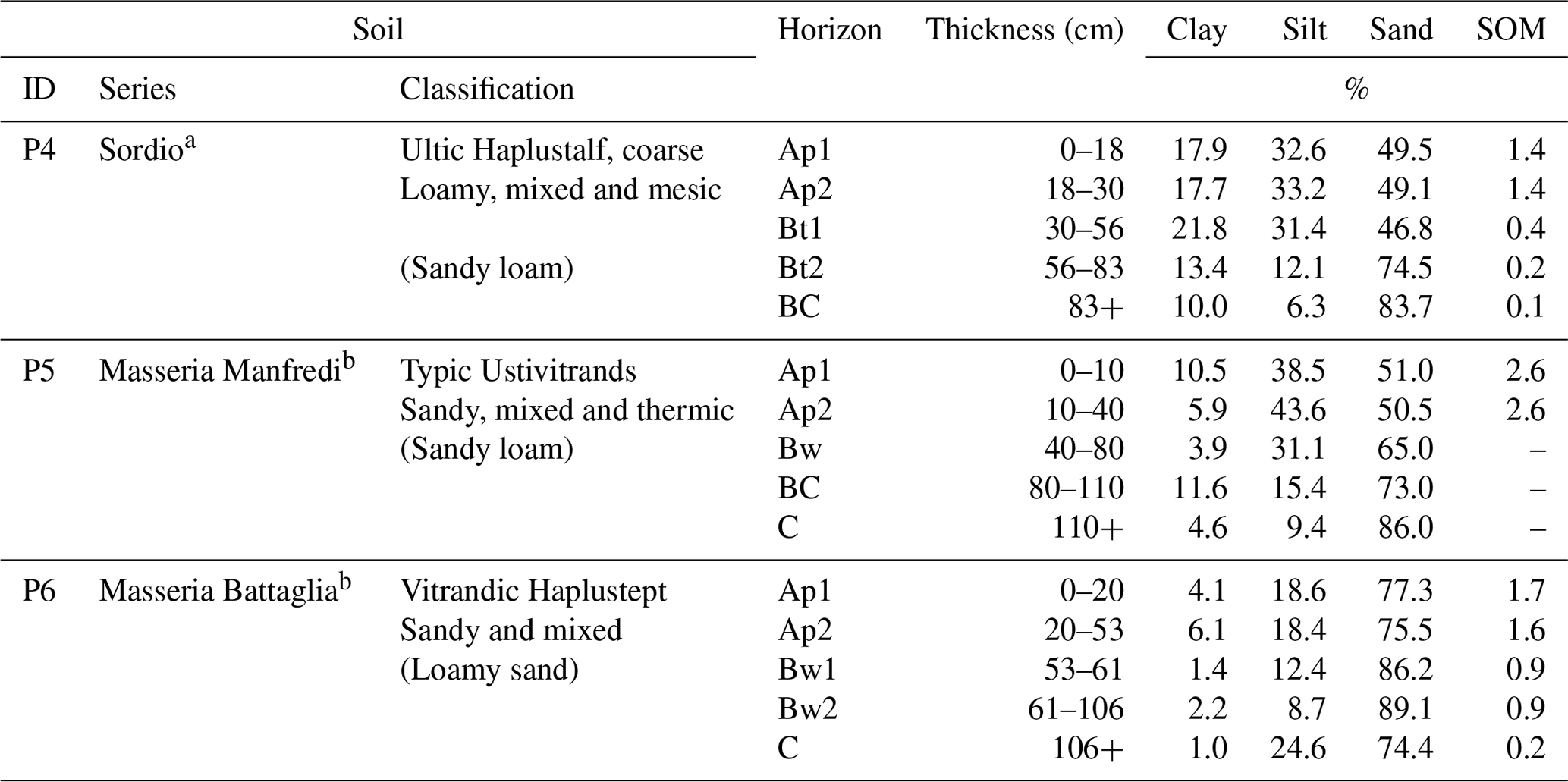
a Soil series from “The soil map of Lodi plain”, 1:37 500 (Huyzendveld and Di Gennaro, 2000). b Close to the soil series of “The soil map of province of Naples”, 1:75 000 (Di Gennaro et al., 1999).
2.3.1 Soil characteristics
The Italian soils are located in a plain in an alluvial environment, with two in the Campania region (P5 and P6) and one (P4) in the Lombardy region. The physical properties of the three selected soils are presented in Table 1. Soil texture ranges from sandy loam to loamy sand, and organic matter contents in the Ap horizons are relatively low, ranging from 1.4 % to 2.6 %, justifying runs for hypothetical contents of 4 %. Based on field observations, the rooting depth of the maize was estimated to be 80 cm, implying that not only the Ap horizon but also subsoil horizons contribute to the water supply to maize.
The soil hydraulic properties applied in the simulation runs, water retention, θ(h), and hydraulic conductivity, k(θ), curves were measured in the laboratory. Undisturbed soil samples (volume ≈ 750 mL) were collected from all of the recognised horizons of the six soil profiles. Samples were slowly saturated from the bottom, and the saturated hydraulic conductivity was measured by a falling head permeameter (Reynolds et al., 2002). Then, both types of θ-h and k-θ data were obtained by means of the evaporation method (Arya, 2002), consisting of an automatic record of the pressure head at three different depths and the weight of the sample during a 1D transient upward flow. From this information, (i) the water retention data θ-h were obtained by applying an iterative method (Basile et al., 2012), and (ii) the unsaturated hydraulic conductivity data were obtained by applying the instantaneous profile method, requiring the spatio-temporal distribution of θ and h, namely θ(z,t) and h(z,t), being z and t, i.e., the depth and time, respectively (Basile et al., 2006). Additional points of the dry branch of the water retention curve were determined using a dew point potentiometer (WP4-T; METER Group, Inc., Washington, USA).
The parameters of the Van Genuchten–Mualem model for water retention and hydraulic conductivity functions were obtained by fitting the experimental θ-h and k-θ data points (Van Genuchten, 1980).
The emphasis in this paper will be on the application of the soil health and soil quality definitions presented above. Initially, three adverse effects of management were considered, namely surface runoff caused by relatively low infiltration rates, erosion of 20 cm of topsoils (while soil classification remains the same) and the formation of a plough pan at 30 cm depth (see Bonfante et al., 2019). Results showed, however, that under prevailing current and future climate conditions surface runoff was negligible. Results will therefore only be presented for phenoforms showing effects of erosion and the plough pan and for increased percentages of OM, as mentioned above.
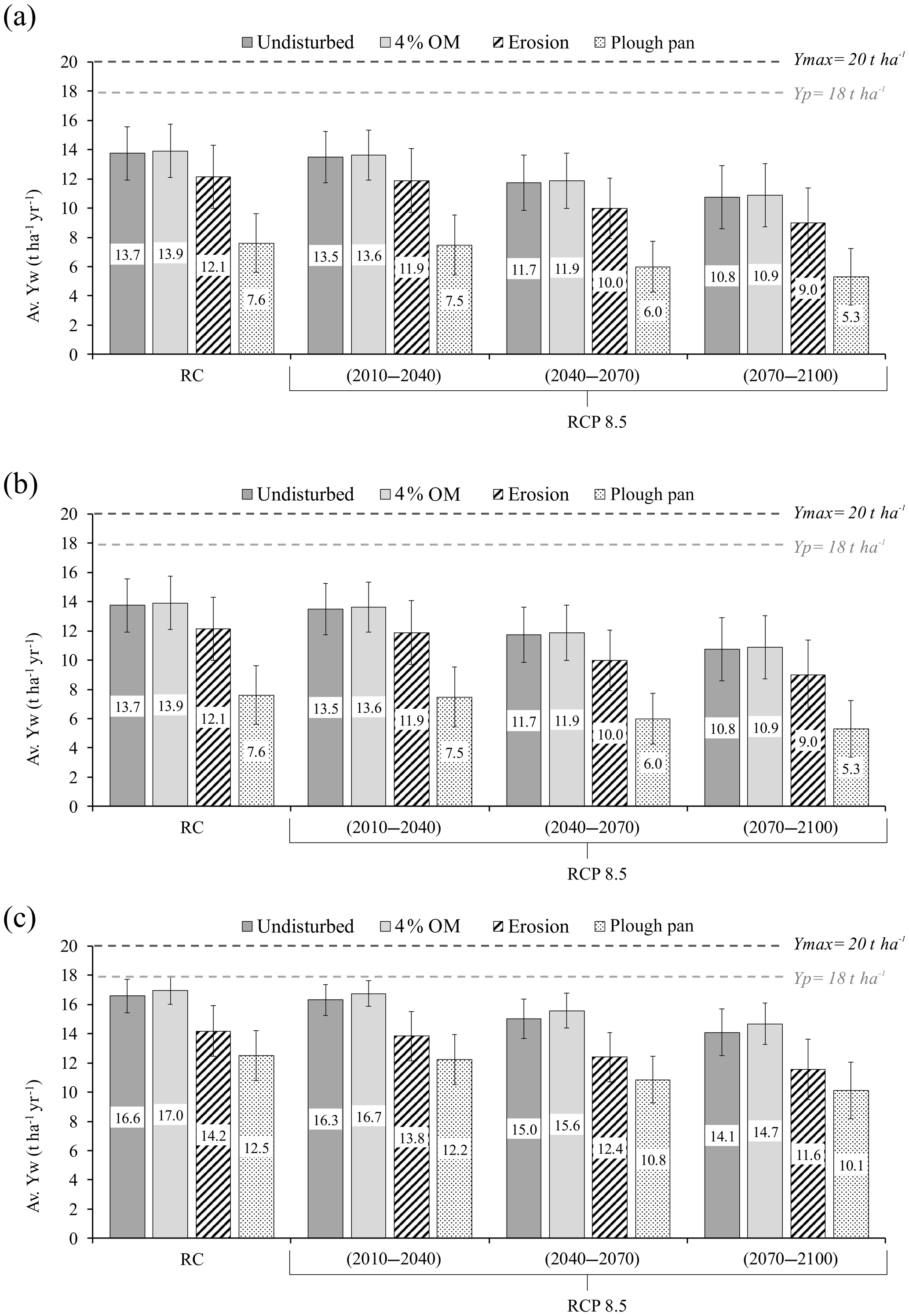
Figure 1The average Yw of four soil phenoforms for three soils, (a) P4, (b) P5 and (c) P6, under reference (RC) and future climate scenarios (RCP 8.5). Yp is the local current potential production, and Ymax is the maximum potential production under unstressed field conditions (i.e. water, nutrients and pests or disease).
3.1 Water-limited yields (Yw)
Water-limited yields (Yw) for four climate periods and three phenoforms for each soil are shown in Fig. 1a for P4, Fig. 1b for P5 and Fig. 1c for P6. Yw values drop for all soils and their phenoforms in the period from the RC to the 2070–2100 climate scenario, particularly for climate scenarios beyond 2040, but, due to relatively high standard deviations, not all differences are significant. However, each soil shows significant drops in Yw for the erosion and plough pan phenoforms, again particularly beyond 2040, when comparing values with Yw undisturbed. Soils P4 and P5 show rather identical behaviour, but soil P6 has significantly higher values for Yw for the erosion and plough pan phenoforms beyond 2040. An increase in percentage OM has a minimal effect, as explained by Bonfante et al. (2020), when considering hydraulic conductivity and moisture retention data.
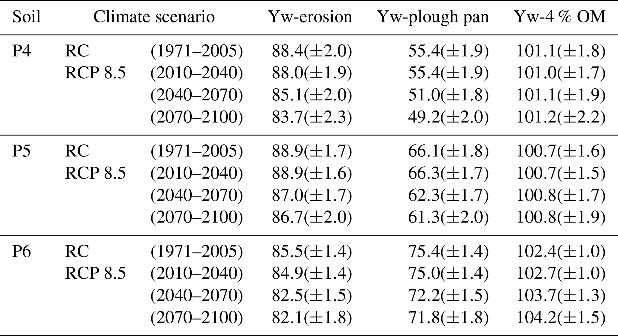
Table 2Soil health (SH) indexes, i.e. (Yw-phenoform/Yw-ref) × 100, defining actual conditions for three selected soils being studied for four climate periods, as indicated. Values are reported for the non-degraded soil and for hypothetical phenoforms representing the erosion of 20 cm of topsoil without a change in soil classification (Yw-erosion) and the occurrence of a plough pan at 30 cm depth (Yw-plough pan). Indexes are also included for hypothetically increased percentages of organic matter (OM) to levels of 4 % (Yw-4 % OM).
3.2 Soil health values for different climate periods
The soil health (SH) index applies to soil health parameter measurements for a given soil at a given time, defining actual conditions, with reference to the particular production potential of the soil type that is present, as expressed by Yw calculated with optimal soil parameters as discussed above. Yw-phenoform conveys conditions expressed by the three soil parameters observed at the site. When Yw-phenoform is equal to Yw, the soil health value will be 100, but this is highly improbable. Lower values indicate room for improvement but offer no information as to factors that lead to these low values (see the next section). Calculated SH indexes for three Italian soil series in four climate periods are reported in Table 2. In this study, four soil conditions were simulated that are common in the field and four climate periods were considered, namely a non-degraded soil characterised by optimal soil parameters (producing Yw-ref) and two Yw-phenoform values, i.e. erosion of topsoil, formation of a plough pan and an increase to 4 % OM. As actual conditions are discussed here, the current climate of 2010–2040 should be considered. Erosion reduces SH to approximately 88, while the plough pan has much stronger effect, with significantly different values of 55 (P4), 66 (P5) and 75 (P6). Increasing the percentage of OM does not deviate from the value of 100, which corresponds with data reported in Fig. 1a–c.
To determine the health index at a given time and place in a given soil, the three soil parameters discussed above are measured, and the model is used to calculate a (Yw-phenoform) value that is then compared with the Yw-ref value calculated with optimal soil parameter values for that particular soil. Management practices that have resulted in the Yw-phenoform being considered should be documented.
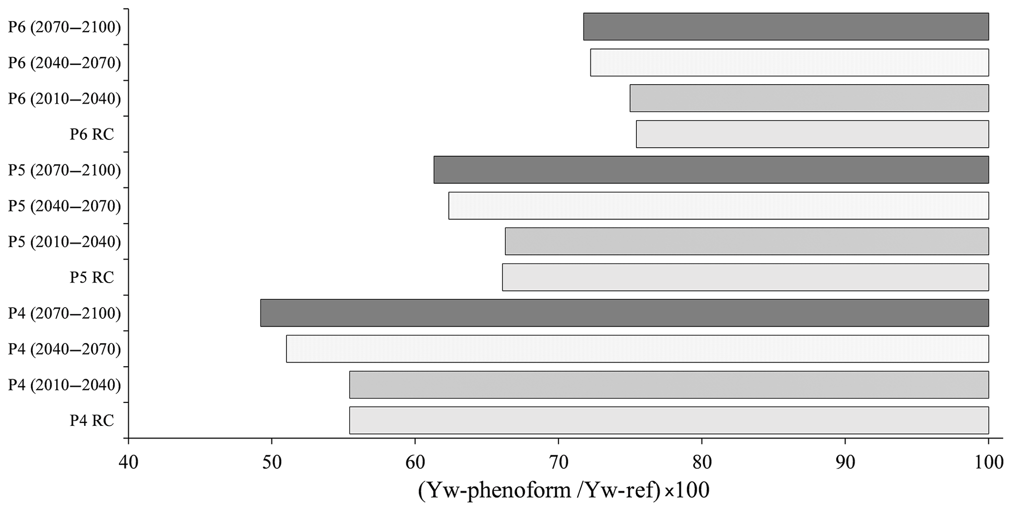
Figure 2Range of soil health indexes – – for the three soils, demonstrating differences among soils and projected effects of climate change. This range characterises the inherent soil quality (SQp) for these particular soil types.
3.3 Soil quality (SQp) in terms of characteristic ranges of soil health values
The SH index, mentioned in the previous section, characterises soil health at a given time and location, as measured in a particular soil type. A gap may become obvious between Yw-phenoform and Yw-ref, but it is not clear what can be done to close the gap. Soil health values for a given soil series can also be obtained at different locations in the same climate zone in which different forms of management have resulted in different phenoforms representing a characteristic range of values that can be seen as a measure for inherent soil quality (SQp). Figure 2 shows a range of values obtained for a given soil type assuming, in this case, the occurrence of only three phenoforms. This only illustrates a principle, and many observations in the field can and should extend the number of points for Yw-phenoform. This range offers a point of reference for each observation, as discussed in the previous section, and allows conclusions regarding advisable management procedures associated with the different phenoforms that, together, determine the observed ranges in Fig. 2.
Figure 2 shows a decreasing sensitivity to soil degradation moving from soil P4 to soil P6. Soil health ratios change from 56 (P4) and 66 (P5) to 78 (P6). The effects of climate change on the index are, again, strongest for soil P4. Figure 2 shows that not only are the ranges of the health index significantly different for the three soils but also their resilience to climate change. A particular soil health measurement in a given soil, as described in the previous section, can now be placed into the bars shown in Fig. 2, indicating possible room for improvement. As every measurement is combined with an assessment of soil use and management that has resulted in the particular phenoform being observed, the system allows the generation of useful management information for the land user.
Table 3SQr index ((Yw/Yp) × 100) for the three selected soils and the four climate periods. Yp is assumed to be 18 tons ha−1.
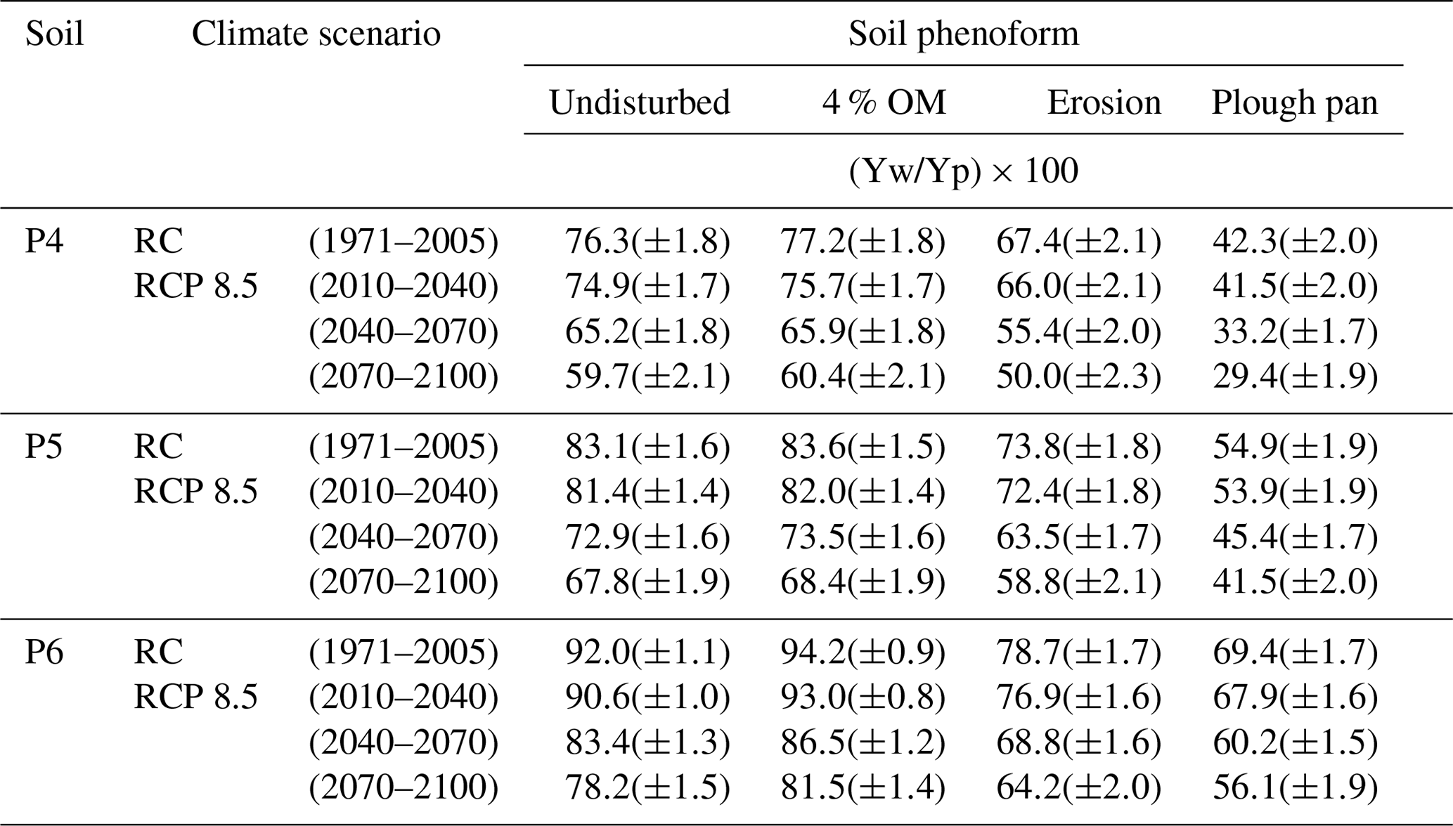
3.4 Comparing different soils in a given region (SQr)
So far, particular soil types have been considered. The analysis can be extended to all soils in a given region and climate zone, and this comparison of different soils can be valuable for regional land use planning. This requires the definition of Yp for the area that is used for the simulations. For the Italian soils being considered, Yp = 18 tons ha−1, and this value is maintained for all climate scenarios considered, implicitly assuming that other factors affecting biomass production will not change. Table 3 shows significant differences among the soils, providing a valuable quantitative assessment. Differences are maintained when different climate periods are considered. Soil P4 scores the lowest values again, with soil P5 scoring intermediate values and soil P6 with the highest values, but even this soil has a low score of 50 for the last climate period when a plough pan is present.
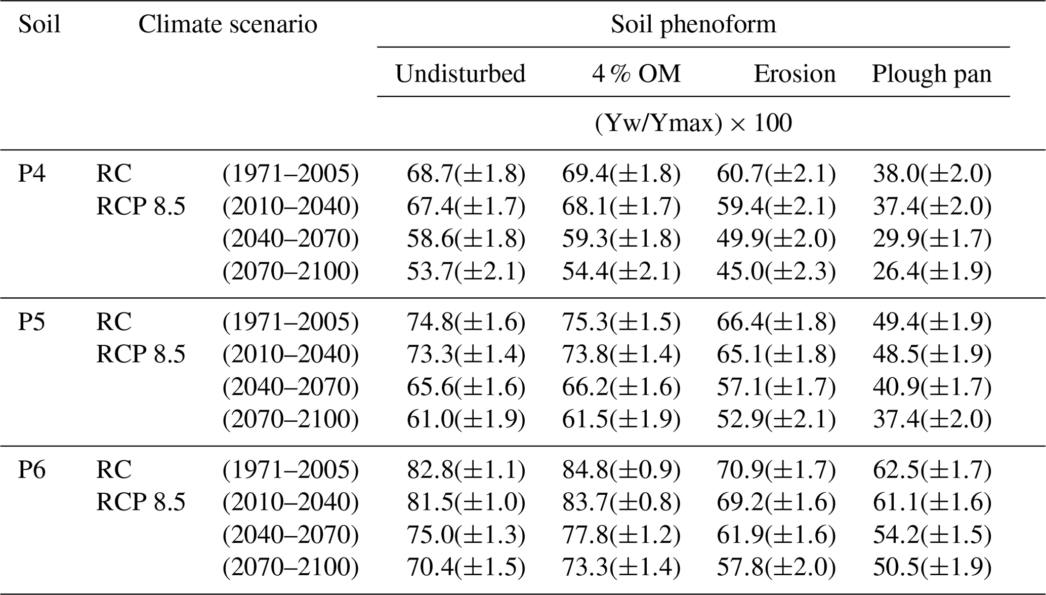
3.5 How to assess soil quality (SQw) in a global context?
Questions about potential food production in future, considering the effects of climate change, require a mechanism for comparing different soils in the world in their capacity to produce biomass. Assuming a maximum production to be achieved in the world (Ymax), considering theoretical photosynthesis under particular climate conditions, values of Yp and Yw can be expressed as a function of Ymax. Use of Yw will produce the most realistic values in view of the limited water availability in many areas of the world. Areas with relatively high values have a higher potential than areas with low values, and this analysis can be helpful input from soil science, contributing to global food production scenarios. Based on current evaluations, a Ymax of 20 tons ha−1 is used here as a reference, and this results in SQw values that can also be expressed for various phenoforms, showing the effects of different forms of degradation Table 4. As in Table 3, differences between the three soils are significant. How these values are to be judged will depend on comparable values assembled for other areas of the world.
Table 4SQw index, (Yw/Ymax) × 100, for the three selected soils and the four climate periods. Ymax is assumed to be 20 tons ha−1.
The soil health concept, as defined in the literature and as modified in this study, is inadequate to allow a comparison of the capacity of different soils to function. Two soils may be healthy in their own way, but a healthy clay soil has a significantly different capacity to function as compared with a healthy sandy soil. As discussed, the soil quality concept can be based on the range of soil health values observed within a given soil type, thus allowing the distinction of differences among different soil types and effects of management. Rather than separating soils in very broad textural classes, we advocate the use of specific soil types as carriers of information (“pedotransfer functions”; Van Looy et al., 2017; Bouma, 2020). Still, the soil health concept is relevant and suitable for expressing the actual condition of a given soil by comparing Yw-phenoform with Yw-ref, as discussed in this paper, producing a soil health index (SH) which follows a procedure that is applied to all soils in the same way.
Of course, Yw assumes real soil water regimes and well-fertilised conditions without pests and diseases. Most often, real yields (Ya) are lower than Yw, and reasons will have to be investigated to select proper soil management. Clearly, different soils often occur within fields, and this will call for precision techniques. This aspect is, however, beyond the scope of this paper.
The advantage of the quantitative procedure for assessing SH and SQ is its basis in a quantitative and reproducible scientific analysis of the plant production process as a function of soil moisture regimes, which is made possible by applying soil–water–atmosphere–plant simulation models. Yw-ref and Yw-phenoform reflect the impact of soil conditions on Ya, the measured yield, as water and nutrients are assumed to be optimal and pests and diseases do not occur. Observing the difference between Ya, on the one hand, and Yw-phenoform and Yw-ref, on the other, can result in fruitful interactions between soil scientists and agronomists who are applying a common language as an effective means of communication.
When applied to three Italian soils, defined by soil classification in terms of three soil series (genoforms), a range of values is obtained not only for an undisturbed soil but also for soils affected by poor forms of soil management, resulting in erosion and compaction (two phenoforms), and (a third phenoform) under good management that increases percentage OM. All of these phenoforms still maintain their genoform classification (Bouma, 1989; Rossiter and Bouma, 2018). In this study, the effects of only three hypothetical phenoforms were explored. In future, field work is required to distinguish a number of characteristic phenoforms for every genoform as a function of current and past soil management. Existing soil maps can be used to identify sampling spots (e.g. Pulleman et al., 2000; Sonneveld et al., 2002).
Again, the different soils show significantly different behaviour, and the ranges for each soil series, reflecting the effects of management, are different. This range represents an inherent property of the soil series being considered, and it is de facto a measure for soil quality (SQp), as expressed in Fig. 2. It adds an important element to soil survey interpretations that are now empirical and qualitative in terms of “general suitabilities or limitations for various forms of land use” (e.g. Bouma, 2020). This requires that properties of phenoforms are explained in terms of management practices. In this context, Pulleman et al. (2000) and Sonneveld et al. (2002) successfully correlated present and past management with the percentage of OM in topsoil.
When considering the use of soils in a given region, the SQr, defined above, is helpful for comparing the production potential of different soils in that particular region.
Finally, analyses on the world level can be made by considering the SQw index, expressing local Yw-ref values (if so desired they can be subdivided in terms of relevant phenoform values) versus a global upper limit. This could be a valuable absolute procedure for comparing soils on a world level, which may be relevant when considering future world food supply scenarios, allowing a focus on potentially favourable locations, providing an added value to the yield gap programme that focuses on reducing the gap (van Ittersum et al., 2013).
The link between soil health and soil quality and primary production allows a direct link with economic aspects (e.g. Priori et al., 2019), while consideration of other ecosystem services allows the consideration of environmental aspects associated with production.
However, as stated in the introduction, soil health and soil quality are not objectives in themselves. Achieving the UN Sustainable Development Goals and the goals of the EU Green Deal require that soils provide effective contributions to various ecosystem services that, in turn, contribute to SDGs and the EU Green Deal. Soils function in an interdisciplinary context, and the implicit hypothesis of soil health assumes that healthy soils will make better contributions to ecosystem services than unhealthy or low quality soils in a regional and world context. But a healthy soil can still make a poor contribution to ecosystem services when poorly managed, illustrating the overriding importance of the management factor.
The application of soil–water–atmosphere–plant models is focused on the ecosystem service of biomass or primary production. However, at the same time, other services have to be provided as well, as discussed earlier, namely water quality protection, reduction of greenhouse gas emissions, carbon capture and biodiversity preservation. Here, applying appropriate management is crucial, and in contrast to the calculations of biomass production, there is no underlying basic theory for identifying options. That is why defining a characteristic range of soil health values for any given soil type as a measure for inherent soil quality (SQp) is important; it will link the land user with experiences obtained elsewhere of similar soils in the same climate zone.
The findings of this paper are as follows:
-
Focusing on actual conditions, when defining soil health, and on inherent conditions, when defining soil quality, allows for a meaningful distinction between the two concepts that are both needed.
-
Introducing the terminology of the agronomic yield gap programme allows quantitative and reproducible expressions for the soil health and soil quality concepts. The distinction of Yw-ref and Yw-phenoform allows independent estimates of soil contributions to Ya, which is the actual yield (= ecosystem service: biomass production) that is determined by many factors other than the soil (e.g. insect invasions, plant diseases, etc.). Applying the yield gap terminology will also facilitate important interactions with agronomists.
-
Emphasising the societal relevance of soil health and soil quality concepts shows that they contribute to defining ecosystem services that, in turn, contribute to the UN SDGs and the EU Green Deal.
-
Demonstrating that soil types were effective carriers of information (class–pedotransfer functions) helped show distinctly different values for the soils being considered.
-
Highlighting the effects of climate change for the Italian soils being considered showed that there is a significant and large reduction in Yw for all degraded and non-degraded scenarios and that agriculture may not be economically viable by the end of the 21st century if irrigation is not feasible.
-
Showing that even healthy soils can fail to make significant contributions to ecosystem services when poor management is applied. Soil use and management play a key role in the interpretation of soil health and soil quality indexes by providing advice as to how to increase indexes. The effects of soil use and management on a given type of soil (genoform) can be expressed by defining phenoforms of particular genoforms. This will require new fieldwork that can be focused by using existing soil maps.
The weather data applied for the simulation run are available online at https://doi.org/10.5281/zenodo.4043286 (last access: 25 September 2020, Bonfante, 2020).
ABo contributed the soil data, simulation results, writing the original draft and the review and editing of the paper. ABa contributed to the soil data, simulation run analysis and writing, and JB suggested the study and contributed to data analysis, writing of the original draft and the review.
The authors declare that they have no conflict of interest.
We acknowledge Nadia Orefice and Roberto De Mascellis for the soil hydraulic property measurements and Eugenia Monaco for her support in the analysis of climate scenarios. Climate data from the Regional Models and geo-Hydrogeological Impacts Division (REMHI) of the Euro-Mediterranean Center on Climate Change (CMCC), Capua, Caserta, Italy, were applied in this study, with support from Paola Mercogliano and Edoardo Bucchignani. Finally, our special thanks to Guido Rianna for the climate data analysis support.
This research has been supported by the EC H2020 LANDSUPPORT project (grant no. 774234).
This paper was edited by Raúl Zornoza and reviewed by two anonymous referees.
Arya, L. M.: Wind and hot-air methods, in: Physical Methods, Soil Science Society of America, Inc., 916–926, 2002.
Basile, A., Coppola, A., De Mascellis, R., and Randazzo, L.: Scaling approach to deduce field unsaturated hydraulic properties and behavior from laboratory measurements on small cores, Vadose Zo. J., 5, 1005–1016, https://doi.org/10.2136/vzj2005.0128, 2006.
Basile, A., Buttafuoco, G., Mele, G., and Tedeschi, A.: Complementary techniques to assess physical properties of a fine soil irrigated with saline water, Environ. Earth Sci., 66, 1797–1807, https://doi.org/10.1007/s12665-011-1404-2, 2012.
Baveye, P. C.: Bypass and hyperbole in soil research: Worrisome practices critically reviewed through examples, Eur. J. Soil Sci., 1–20, https://doi.org/10.1111/ejss.12941, 2020.
Bonfante, A. and Bouma, J.: The role of soil series in quantitative land evaluation when expressing effects of climate change and crop breeding on future land use, Geoderma, 259, 187–195, 2015.
Bonfante, A., Terribile, F., and Bouma, J.: Refining physical aspects of soil quality and soil health when exploring the effects of soil degradation and climate change on biomass production: an Italian case study, SOIL, 5, 1–14, https://doi.org/10.5194/soil-5-1-2019, 2019.
Bonfante, A., Basile, A., and Bouma, J.: Exploring the effect of varying soil organic matter contents on current and future moisture supply capacities of six Italian soils, Geoderma, 361, 114079, https://doi.org/10.1016/j.geoderma.2019.114079, 2020.
Bonfante, A.: Reference Climate (1971–2005) and RCP8.5 scenario (2010–2100) of Destra sele for SWAP simulation, available at: https://doi.org/10.5281/zenodo.4043286, last access: 25 September 2020.
Bouma, J.: Using Soil Survey Data for Quantitative Land Evaluation, Springer, New York, NY, 177–213, 1989.
Bouma, J.: Soil science contributions towards sustainable development goals and their implementation: linking soil functions with ecosystem services, J. Plant Nutr. Soil Sci., 177, 111–120, 2014.
Bouma, J.: Comment on: B. Minasny and A. B. Mc Bratney. 2018, Limited effect of organic matter on soil available water capacity, Eur. J. Soil Sci., 69, 154–154, https://doi.org/10.1111/ejss.12509, 2018.
Bouma, J.: Contributing pedological expertise towards achieving the United Nations Sustainable Development Goals, Geoderma, 375, 114508, https://doi.org/10.1016/j.geoderma.2020.114508, 2020.
Bucchignani, E., Montesarchio, M., Zollo, A. L., and Mercogliano, P.: High-resolution climate simulations with COSMO-CLM over Italy: performance evaluation and climate projections for the 21st century, Int. J. Climatol., 36, 735–756, 2015.
Bünemann, E. K., Bongiorno, G., Bai, Z., Creamer, R. E., De Deyn, G., de Goede, R., Fleskens, L., Geissen, V., Kuyper, T. W., Mäder, P., Pulleman, M., Sukkel, W., van Groenigen, J. W., and Brussaard, L.: Soil quality – A critical review, Soil Biol. Biochem., 120, 105–125, https://doi.org/10.1016/j.soilbio.2018.01.030, 2018.
Droogers, P. and Bouma, J.: Soil survey input in exploratory modeling of sustainable soil management practices, Soil Sci. Soc. Am. J., 61, 1704–1710, 1997.
Duda, B. M., Weindorf, D. C., Chakraborty, S., Li, B., Man, T., Paulette, L., and Deb, S.: Soil characterization across catenas via advanced proximal sensors, Geoderma, 298, 78–91, https://doi.org/10.1016/j.geoderma.2017.03.017, 2017.
European Commission (EC): Communication from the Commission to the Council, the European Parliament, the European Economic and Social Committee and the Committee of the Regions, Thematic Strategy for Soil Protection, COM 231 Final, Brussels, Belgium, 12 pp., 2006.
Feddes, R. A., Kowalik, P. J., and Zaradny, H.: Simulation of field water use and crop yield, Centre for Agricultural Publishing and Documentation, 189 pp., 1978.
Hack-ten Broeke, M. J. D., Mulder, H. M., Bartholomeus, R. P., van Dam, J. C., Holshof, G., Hoving, I. E., Walvoort, D. J. J., Heinen, M., Kroes, J. G., van Bakel, P. J. T., Supit, I., de Wit, A. J. W., and Ruijtenberg, R.: Quantitative land evaluation implemented in Dutch water management, Geoderma, 338, 536–545, https://doi.org/10.1016/j.geoderma.2018.11.002, 2019.
Hargreaves, G. H. and Samani, Z. A.: Reference crop evapotranspiration from temperature, Appl. Eng. Agric., 1, 96–99, 1985.
Holzworth, D., Huth, N. I., Fainges, J., Brown, H., Zurcher, E., Cichota, R., Verrall, S., Herrmann, N. I., Zheng, B., and Snow, V.: APSIM Next Generation: Overcoming challenges in modernising a farming systems model, Environ. Model. Softw., 103, 43–51, https://doi.org/10.1016/j.envsoft.2018.02.002, 2018.
IPCC: Climate Change 2014, – Impacts, Adaptation and Vulnerability: Regional Aspects, edited by: Field, Christopher B., Cambridge University Press, 1783 pp., 2014.
Keesstra, S. D., Bouma, J., Wallinga, J., Tittonell, P., Smith, P., Cerdà, A., Montanarella, L., Quinton, J. N., Pachepsky, Y., van der Putten, W. H., Bardgett, R. D., Moolenaar, S., Mol, G., Jansen, B., and Fresco, L. O.: The significance of soils and soil science towards realization of the United Nations Sustainable Development Goals, SOIL, 2, 111–128, https://doi.org/10.5194/soil-2-111-2016, 2016. Kroes, J. G., Van Dam, J. C., Bartholomeus, R. P., Groenendijk, P., Heinen, M., Hendriks, R. F. A., Mulder, H. M., Supit, I., and Van Walsum, P. E. V: Theory description and user manual SWAP version 4, available at: http://www.swap.alterra.nl, Wageningen [online], available from: http://www.wur.eu/environmental-research (last access: 24 July 2019), 2017.
Ma, L., Ahuja, L. R., Nolan, B. T., Malone, R. W., Trout, T. J., and Qi, Z.: Root zone water Quality Model (RZWQM2): model use, calibration and validation, Trans. ASABE., 55, 1424–1446, https://doi.org/10.13031/2013.42252, 2012.
Meinshausen, M., Smith, S. J., Calvin, K., Daniel, J. S., Kainuma, M. L. T., Lamarque, J., Matsumoto, K., Montzka, S. A., Raper, S. C. B., Riahi, K., Thomson, A., Velders, G. J. M. and van Vuuren, D. P. P.: The RCP greenhouse gas concentrations and their extensions from 1765 to 2300, Clim. Change, 109, 213–241, doi:10.1007/s10584-011-0156-z, 2011.
Moebius-Clune, B. N., Moebius-Clune, D. J., Gugino, B. K., Idowu, O. J., Schindelbeck, R. R., Ristow, A. J., van Es, H. M., Thies, J. E., Shayler, H. A., McBride, M. B., Kurtz, K. S. M., Wolfe, D. W., and Abawi, G. S.: Comprehensive assessment of soil health: The Cornell Framework Manual, Edition 3.1, Cornell Univ., Ithaca, NY, 2016.
Orgiazzi, A., Ballabio, C., Panagos, P., Jones, A., and Fernández-Ugalde, O.: LUCAS Soil, the largest expandable soil dataset for Europe: a review, Eur. J. Soil Sci., 69, 140–153, 2018.
Norris, C. E., MacBean, G., Cappellazi, S. B., Cope, M., Greub, K. L. H., Liptzin, D., Rieke, E. L., Tracy, P. W., Morgan, C. L. S., and Honeycutt, C. W.: Introducing the North American project to evaluate soil health measurements, Agronomy Journal, 112, 3195–3215, https://doi.org/10.1002/agj2.20234, 2020.
Pulleman, M. M., Bouma, J., Van Essen, E. A., and Meijles, E. W.: Soil organic matter content as a function of different land use history, Soil Sci. Soc. Am. J., 64, 689–693, 2000.
Priori, S., Fantappiè, M., Bianconi, N., Ferrigno, G., Pellegrini, S., and Costantini, E. A. C.: Field-Scale Mapping of Soil Carbon Stock with Limited Sampling by Coupling Gamma-Ray and Vis-NIR Spectroscopy, Soil Sci. Soc. Am. J., 80, 954–964, https://doi.org/10.2136/sssaj2016.01.0018, 2016.
Priori, S., Barbetti, R., Meini, L., Morelli, A., Zampolli, A., and D'Avino, L.: Towards Economic Land Evaluation at the Farm Scale Based on Soil Physical-Hydrological Features and Ecosystem Services, Water, 11, 1527, https://doi.org/10.3390/w11081527, 2019.
Reynolds, M., Kropff, M., Crossa, J., Koo, J., Kruseman, G., Molero Milan, A., Rutkoski, J., Schulthess, U., Balwinder-Singh, S. K., Tonnang, H., Vadez, V., Reynolds, M., Kropff, M., Crossa, J., Koo, J., Kruseman, G., Molero Milan, A., Rutkoski, J., Schulthess, U., Balwinder-Singh, Sonder, K., Tonnang, H., and Vadez, V.: Role of Modelling in International Crop Research: Overview and Some Case Studies, Agronomy, 8, 291, https://doi.org/10.3390/agronomy8120291, 2018.
Reynolds, W. D., Elrick, D. E., Youngs, E. G., Booltink, H. W. G., Bouma, J., and Dane, J. H.: Saturated and field-saturated water flow parameters. 2. Laboratory methods, available at: http://agris.fao.org/agris-search/search.do?recordID=NL2003682903, (last acccess: 28 January 2019), 2002.
Ritchie, J. T.: Model for predicting evaporation from a row crop with incomplete cover, Water Resour. Res., 8, 1204–1213, 1972.
Rockel, B., Will, A., and Hense, A.: The regional climate model COSMO-CLM (CCLM), Meteorol. Z., 17, 347–348, 2008.
Rossiter, D. G. and Bouma, J.: A new look at soil phenoforms–Definition, identification, mapping, Geoderma, 314, 113–121, 2018.
Sonneveld, M. P. W., Bouma, J., and Veldkamp, A.: Refining soil survey information for a Dutch soil series using land use history, Soil Use Manag., 18, 157–163, https://doi.org/10.1111/j.1475-2743.2002.tb00235.x, 2002.
Steduto, P., Hsiao, T. C., Fereres, E., and Raes, D.: Crop yield response to water, FAO Roma, 500 pp., 2012.
USDA: National Resources Conservation Services (NRCS) of the US Dept. Agric. Soil Health, available at: https://www.nrcs.usda.gov/wps/portal/nrcs/main/soils/health/ (last access: 25 September 202), 2019.
van Ittersum, M. K., Cassman, K. G., Grassini, P., Wolf, J., Tittonell, P., and Hochman, Z.: Yield gap analysis with local to global relevance a review, F. Crop. Res., 143, 4–17, 2013.
Van Genuchten, M. T.: A closed-form equation for predicting the hydraulic conductivity of unsaturated soils, Soil Sci. Soc. Am. J., 44, 892–898, 1980.
Van Looy K., Bouma J., Herbst M., Koestel J., Minasny B., Mishra U., Montzka C., Nemes A., Pachepsky, Y., Padarian J., Schaap, M., Tóth, B., Verhoef, A., Vanderborght, J., van der Ploeg, M., Weihermüller, L., Zacharias, S., Zhang, Y., and Vereecken, H.: Pedotransfer functions in Earth system science: challenges and perspectives., Rev. Geophys., 55, 1199–1256, https://doi.org/10.1002/2017RG000581, 2017.
White, J. W., Hunt, L. A., Boote, K. J., Jones, J. W., Koo, J., Kim, S., Porter, C. H., Wilkens, P. W., and Hoogenboom, G.: Integrated description of agricultural field experiments and production: The ICASA Version 2.0 data standards, Comput. Electron. Agric., 96, 1–12, https://doi.org/10.1016/j.compag.2013.04.003, 2013.
Zollo, A. L., Turco, M., and Mercogliano, P.: Assessment of hybrid downscaling techniques for precipitation over the Po river basin, in: Engineering Geology for Society and Territory-Volume 1, Springer, 193–197, 2015.