the Creative Commons Attribution 4.0 License.
the Creative Commons Attribution 4.0 License.
 | 14 Jul 2020
Oblique geographic coordinates as covariates for digital soil mapping
Anders Bjørn Møller
Amélie Marie Beucher
Nastaran Pouladi
Mogens Humlekrog Greve
Decision tree algorithms, such as random forest, have become a widely adapted method for mapping soil properties in geographic space. However, implementing explicit spatial trends into these algorithms has proven problematic. Using x and y coordinates as covariates gives orthogonal artifacts in the maps, and alternative methods using distances as covariates can be inflexible and difficult to interpret. We propose instead the use of coordinates along several axes tilted at oblique angles to provide an easily interpretable method for obtaining a realistic prediction surface. We test the method on four spatial datasets and compare it to similar methods. The results show that the method provides accuracies better than or on par with the most reliable alternative methods, namely kriging and distance-based covariates. Furthermore, the proposed method is highly flexible, scalable and easily interpretable. This makes it a promising tool for mapping soil properties with complex spatial variation.
- Article
(9630 KB) - Full-text XML
- BibTeX
- EndNote


Machine learning has become a frequently applied means for mapping soil properties in geographic space. The most common approach is to train models from soil observations and covariates in the form of geographic data layers. The models can often provide reliable predictions of soil properties. Many researchers have used decision tree algorithms as they are computationally efficient, do not rely on assumptions about the distributions of the input variables, and can use both numeric and categorical data (Quinlan, 1996; Mitchell, 1997; Rokach and Maimon, 2005; Tan et al., 2014). Additionally, they effectively handle nonlinear relationships and complex interactions (Strobl et al., 2009).
However, a disadvantage of decision tree models is that they do not explicitly take into account spatial trends in the data. Unlike geostatistical methods, such as kriging, the predictions can therefore contain spatial bias.
A number of studies have applied regression kriging (RK) as a solution (Knotters et al., 1995; Odeh et al., 1995; Hengl et al., 2004). By kriging the residuals of the predictive model and adding the kriged residuals to the prediction surface, this approach can account for spatial trends and achieve higher accuracies. A disadvantage of RK is that the combination of two models hinders the combination of spatial trends with the other covariates. Spatial trends therefore remain disconnected from other statistical relationships in the analysis, leading to difficulties in interpreting the model and its associated uncertainties.
An obvious solution to this problem would be to use the x and y coordinates of the soil observations as covariates. However, results have shown that this approach can lead to unrealistic orthogonal artifacts in the output maps when used in conjunction with decision tree algorithms (Behrens et al., 2018; Hengl et al., 2018; Nussbaum et al., 2018). The cause of this problem lies in the splitting procedure of decision tree algorithms, as they use only one covariate for each split. Therefore, a dataset containing only the x and y coordinates will force the algorithm to make orthogonal splits in geographic space.
Several researchers have proposed solutions to this problem. Behrens et al. (2018) proposed the use of Euclidean distance fields (EDFs) in the form of distances to the corners and middle of the study area and the x and y coordinates. Their results showed that this approach efficiently integrated spatial trends and that accuracies were better than or on par with other methods for integrating spatial context.
On the other hand, Hengl et al. (2018) suggested an approach referred to as spatial random forest (RFsp). This method consists of calculating data layers with buffer distances to each of the soil observations in the training dataset. It then trains a random forest model, using the buffer distances as covariates, either combined with auxiliary data or on their own. One of the main advantages of this approach is that it incorporates distances between observations in a similar manner to geostatistical models. The authors assessed the use of RFsp on a large number of spatial prediction problems and showed that it effectively eliminated spatial trends in the residuals.
Although these two methods are able to integrate spatial trends in machine-learning models, they can be difficult to interpret. The distances used in EDFs depend on the geometry of the study area, and for RFsp, they depend on the locations of the soil samples. The meaning and interpretation of the distances therefore varies depending on the study area and the soil observations.
EDFs and RFsp also have limited flexibility as both methods specify the number of geographic data layers a priori. For EDFs, the number of distance fields is seven, and for RFsp, the number of buffer distances is equal to the number of soil observations. This means that there is no straightforward way to increase the number of spatially explicit covariates if the number is insufficient to account for spatial trends. Conversely, there is no way to decrease the number of spatially explicit covariates, even if a smaller number would suffice. The latter is especially relevant for RFsp as the method is computationally unfeasible for datasets with a large number of observations (Hengl et al., 2018).
In this study, we propose an alternative method for including spatially explicit covariates for mapping soil properties. With the method, we aim to directly address the cause of the orthogonal artifacts produced with x and y coordinates as covariates in decision tree models. Furthermore, we aim to improve upon the shortcomings of previous methods by developing a method that is both flexible and easily interpretable.
We refer to the method as oblique geographic coordinates (OGCs). In short, it works by calculating coordinates for the observations along a series of axes tilted at several oblique angles relative to the x axis. By including oblique coordinates as covariates, we enable the decision tree algorithm to make oblique splits in geographic space. As this is not possible with only x and y coordinates as covariates, this addition should allow the model to produce a more realistic prediction surface. Furthermore, the number of oblique angles is adjustable, and soil mappers can therefore choose a number that suits their purpose. Some mapping tasks may require a higher number of oblique angles than others, and soil mappers can therefore increase the number as necessary. Alternatively, if a small number of oblique angles suffices, soil mappers can reduce their number and thereby shorten computation times.
We test the method on four spatial datasets. Firstly, we test it for predicting soil organic matter contents in a densely sampled agricultural field in Denmark, located in northern Europe. Secondly, we test it on three publicly available spatial datasets (meuse, eberg and Swiss rainfall). We hypothesize that OGCs can provide accuracies on par with previous methods for including explicitly spatial covariates. We also hypothesize that it is possible to adjust the number of oblique angles in order to optimize accuracy and that the results allow for meaningful interpretations.
2.1 Study areas
We test OGCs and compare them to other methods based on four spatial datasets. Firstly, we test them for a predicting soil organic matter (SOM) for an agricultural field in Denmark (Vindum). Secondly, we test them on three publicly available datasets. For Vindum, we will present methods and results in detail. For the other three datasets, we will present methods and results in brief, while Appendix A contains a detailed presentation of the methods and results for these datasets.
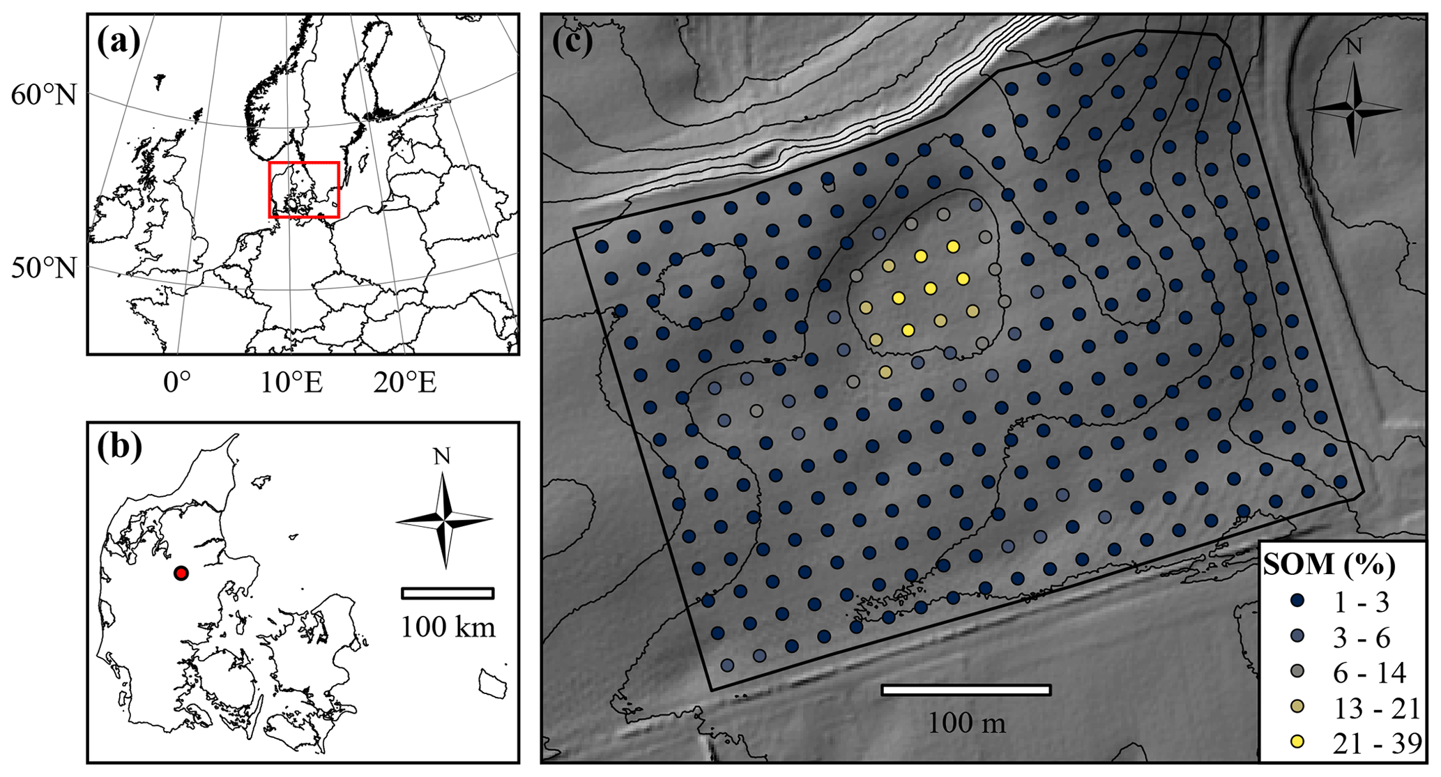
Figure 1(a) Location of Denmark in northern Europe. (b) Location of the Vindum field within Denmark. (c) Map of the Vindum field, including locations of the samples extracted for soil organic matter (SOM) measurements. The thin black lines are 2 m contour lines. The background shows hill shade (northwest; 45∘ altitude) based a digital elevation model (DEM) in 1.6 m×1.6 m resolution (National Survey and Cadastre of Denmark, 2012).
2.1.1 Vindum
This study area is a 12 ha agricultural field located in Denmark in northern Europe (9.568∘ E, 56.375∘ N; European Terrestrial Reference System (ETRS89), 1989; Fig. 1). It lies in a kettled moraine landscape 55–66 m above sea level (a.s.l.). The parent materials in the field include clay till, glaciofluvial sand and peat. The climate is temperate coastal, with mean monthly temperatures ranging from 1 ∘C in January to 17 ∘C in July and a mean annual precipitation of 850 mm (Wang, 2013). The field contains 285 measurements of SOM from the depth interval 0–25 cm located in a 20 m grid.
The SOM contents of the topsoil in the field range from 1.3 % to 38.8 %, with a mean value of 3.5 % and a median of 2.2 %. The values have a strong positive skew of 4.7 and are leptokurtic with a kurtosis of 26.9. Logarithmic transformation reduces skewness (2.9) and kurtosis (11.1). Pouladi et al. (2019) described the spatial structure of the data, with a stable variogram with 139 m range, nugget of 0 and sill of 23.8.
2.1.2 Additional datasets
For additional analyses, we included the meuse dataset, the eberg dataset and the Swiss rainfall dataset. The meuse dataset, available through the R package sp (Pebesma et al., 2020), contains 155 measurements of soil heavy-metal concentrations from a 5 km2 flood plain of the Meuse River near the village of Stein in the Netherlands. For this dataset, we mapped zinc concentrations. The eberg dataset, available through the R package plotKML (Hengl et al., 2020), contains 3670 soil observations from a 100 km2 area in Ebergötzen near the city of Göttingen in Germany. For this dataset, we mapped soil types. Lastly, the Swiss rainfall dataset contains 476 rainfall measurements from 8 May 1986 in Switzerland (Dubois et al., 2003). Although this is not a soil dataset, we included it because of the high anisotropy of the data, which makes it useful for comparing methods on their ability to account for anisotropic spatial problems. We describe these three datasets in more detail in Appendix A.
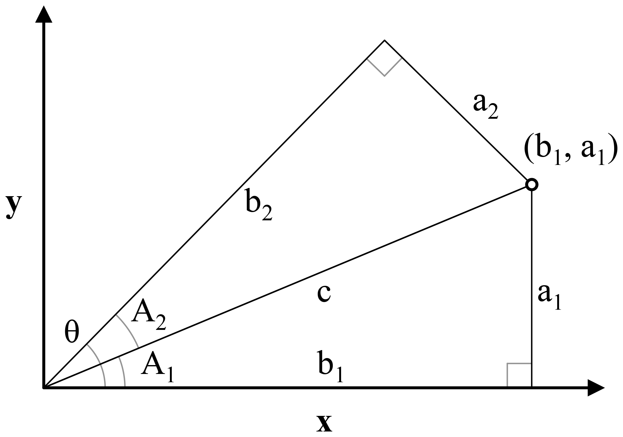
Figure 2Illustration for the derivation of the oblique geographic coordinate for the point (b1, a1) along an axis tilted with the angle θ from the x axis. The coordinate is equal to the length of b2. Triangles a1b1c and a2b2c are right triangles with the same hypotenuse c. The sides a1 and b1 are the x and y coordinates of the point (b1, a1), respectively. A1 is the angle between the x axis and the line c between the origin of the coordinate system and the point (b1, a1); A2 is the difference between θ and A1.
2.2 Oblique geographic coordinates
The method that we propose consists of calculating coordinates along a number of axes titled at various oblique angles, relative to the x axis. In the following, we show that it is possible to calculate the coordinate of a point (b1, a1) along an axis tilted at an angle θ relative to the x axis, based on θ and the x and y coordinates of the point (b1, a1). Equation (1) shows the calculation of the oblique geographic coordinate, using Fig. 2 for illustration.
where θ is the angle of the titled axis relative to the x axis; a1 is the y coordinate of (b1, a1); b1 is the x coordinate of (b1, a1); and b2 (or “OGCs”) is the coordinate of (b1, a1) along an axis tilted with the angle θ relative to the x axis.
As the x and y coordinates of soil observations are known, and θ is given, it is possible to calculate coordinates at oblique angles for all soil observations in a dataset. Likewise, as the x and y coordinates of the cells in a geographic raster layer are known, it is possible to calculate oblique coordinates for the cells. Our approach relies on calculating coordinates along n axes tilted at angles ranging from zero to ) with increments of π∕n between the angles. θ should not be π or greater, as coordinates along axes tilted at these angles will correlate with coordinates along axes tilted at angles of zero to ). For example, coordinates along an axis with θ= 0.25π (northeast) perfectly correlate with coordinates along an axis with θ=1.25π (southwest). Figure 3 shows coordinates along axes tilted at six different angles relative to the x axis for the Vindum study area. The coordinate rasters (a) and (d) are equivalent to the x and y coordinates, respectively, while the coordinate rasters (b), (c), (e) and (f) show coordinates at oblique angles.

Figure 3Examples of rasters with coordinates tilted at six different angles for the Vindum study area. Easting and northing for the Universal Transverse Mercator (UTM) zone 32N (ETRS89).
2.3 Method comparison
2.3.1 Vindum
We use the 285 SOM observations from the Vindum study area in order to test the accuracy of predictions made by random forest models using OGCs as covariates. In addition to OGCs, we also employed 19 data layers with auxiliary data, which Pouladi et al. (2019) derived from a 1.6 m digital elevation model (DEM), satellite imagery and electromagnetic induction. Topographic variables included the sine and cosine of the aspect, depth of sinks, plan and profile curvature, elevation, flow accumulation, valley bottom flatness, midslope position, standard and modified topographic wetness index, slope gradient, slope length, and valley depth. Satellite imagery included normalized difference, absolute difference, ratio and soil-adjusted vegetation indices. Lastly, we used the apparent electrical conductivity from a DUALEM-1 sensor in perpendicular mode.
In order to optimize the number of raster layers for OGCs, we generated datasets with 2–100 coordinate rasters. We then trained random forest models from each dataset, both with and without auxiliary data. In order to assess predictive accuracy, we used 100 repeated splits on the SOM observations, each using 75 % of the observations for model training and a 25 % holdout dataset for accuracy assessment. We trained models using the R package ranger (Wright and Ziegler, 2015) and parameterized the models using the R package caret (Kuhn, 2008). For each split, we tested five different values for mtry, with minimum node sizes of 1, 2, 4 and 8 and two different splitting rules, namely variance and extratrees. We mainly adjusted mtry and the minimum node size in order to avoid overfitting. We tested mtry values at even intervals between 2 and the total number of covariates, including both auxiliary data and spatially explicit covariates. The tested mtry values therefore varied, depending on the number of covariates. The extratrees splitting rule generates random splits as opposed to the variance splitting rule, which chooses optimal splits. By default, extratrees generates one random split for each covariate and then chooses the random split that gives the largest variance reduction (Geurts et al., 2006). It therefore leads to a greater degree of randomization. We selected the setup that provided the lowest root mean square error (RMSE) for the out-of-bag predictions on the training data and used this setup for predictions on the 25 % holdout dataset.
We used the same 100 repeated splits for each number of coordinate rasters, with and without auxiliary data. We calculated accuracy based on Pearson's R2, RMSE and Lin's concordance criterion (ccc) and subsequently used the number of coordinate rasters that yielded the lowest RMSE. We selected a different number of coordinate rasters with and without auxiliary data.
We then compared the accuracies obtained with the optimal numbers of coordinate rasters, with and without auxiliary data, to the accuracies obtained with other methods. We tested kriging, random forest models trained only on the auxiliary data and random forest models trained using EDFs and RFsp, with and without auxiliary data. We trained the random forest models using the same procedure outlined above. For kriging, we used variograms automatically fitted on logarithmic-transformed SOM observations using the autofitVariogram function of the R package automap (Hiemstra, 2013). A previous study using the same dataset showed that kriging predicted SOM more accurately than regression kriging (Pouladi et al., 2019). We therefore omitted regression kriging from the analysis although, without this previous finding, it would have been relevant to include it.
We used the same 100 repeated splits for assessing the accuracies of all methods. This allowed us to carry out pairwise t tests between the accuracies of the methods. We used the results of the pairwise t tests to rank the methods according to their accuracies according to each of the metrics. If there was no statistical difference (p>0.05) between the accuracies of two or more methods, these methods received the same rank. We calculated separate ranks for the methods for each accuracy metric, resulting in three different sets of ranks. In order to illustrate the results, we produced maps of SOM with each method, using models trained from all the data.
We also investigated the covariate importance of models trained with OGCs and tested all methods for spatially autocorrelated residuals using experimental variograms. To produce sample variograms of the residuals, we produced maps with each method using all observations. We converted both observations and predictions to a natural logarithmic scale. We then subtracted the predictions from the observations and calculated variograms for these residuals. For this purpose, we used the function variogram from the R package gstat (Pebesma and Graeler, 2020) with its default parameters.
2.3.2 Additional datasets
We also compared OGCs to other methods based on the three additional datasets meuse, eberg and Swiss rainfall. The methods in the comparison depended on the dataset. For the meuse dataset, we tested all the methods tested on the Vindum dataset, with the addition of RK using random forest models for regression. For the eberg dataset, we tested random forest models based on auxiliary data (AUX), EDFs and OGCs, and the combined methods (EDFs + AUX and OGCs + AUX). For the Swiss rainfall dataset, we tested only purely spatial methods, including ordinary kriging (OK), EDFs, RFsp and OGCs. As for the Vindum dataset, we tested each method based on 100 splits into training and test data and carried out pairwise t tests on the resulting accuracies. Appendix A gives additional details on the methods for each dataset. For the three additional datasets, we focused on the accuracies and maps produced with each method. We therefore omitted analyses of the residuals and covariate importance of these datasets.
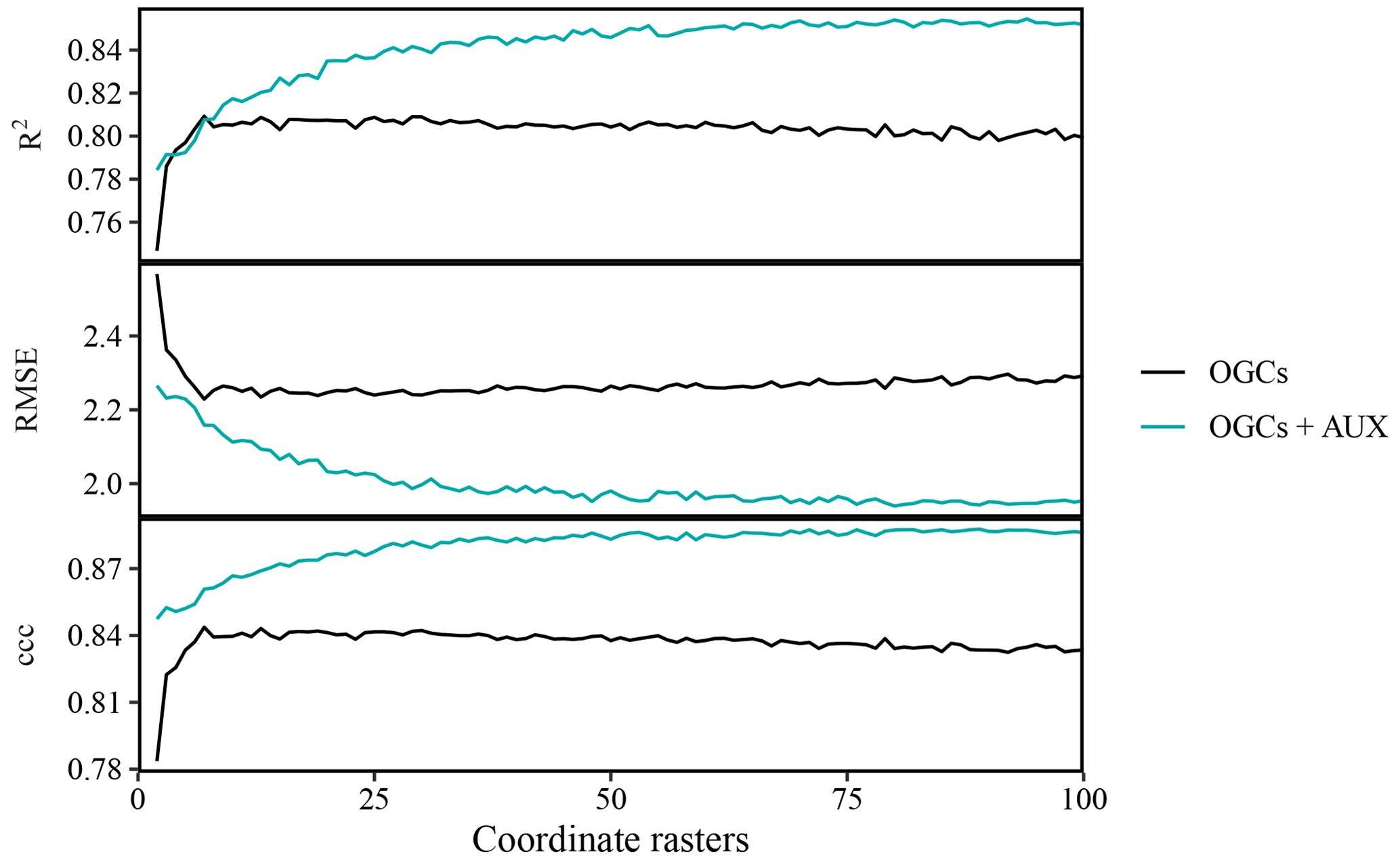
Figure 4Effects of the number of coordinate rasters on the accuracy of SOM predictions on the Vindum dataset, calculated as Pearson's R2, root mean square error (RMSE) and Lin's concordance criterion (ccc). We calculated effects for random forest models trained on only coordinate rasters (OGCs) and with coordinate rasters in combination with auxiliary data (OGCs + AUX). The lines represent mean values obtained from 100 repeated splits (75 % training dataset; 25 % test dataset) for each number of coordinate rasters.
3.1 Optimal number of coordinate rasters
3.1.1 Vindum
For the Vindum dataset, accuracies of predictions obtained with OGCs, without auxiliary data, increased with the number of coordinate rasters up to an optimum at seven coordinate rasters (Fig. 4). However, with more than seven coordinate rasters, accuracies deteriorated slightly with the number of coordinate rasters. This pattern was the same for all three metrics. On the other hand, with OGCs in combination with auxiliary data, accuracies generally increased with the number of coordinate rasters. The increase was greatest when the number of coordinate rasters was small, while the effect of more coordinate rasters decreased for larger numbers of coordinate rasters. With auxiliary data, the optimal number of coordinate rasters was 94 for Pearson's R2, 80 for RMSE and 89 for ccc. Accuracies with auxiliary data were almost invariably higher than accuracies achieved without auxiliary data.

Figure 5Maps of soil organic matter (SOM) contents in the topsoil at Vindum predicted using random forest models trained with coordinate rasters at two to seven different angles as covariates. Easting and northing for UTM zone 32N (ETRS89).
Figure 5 shows SOM contents mapped for Vindum with increasing numbers of coordinate rasters, without auxiliary data. The predictions with only two coordinate rasters showed a pattern very typical of predictions with x and y coordinates with very visible orthogonal artifacts. As the number of coordinate rasters increased, the patterns of the artifacts changed. With coordinate rasters at three different angles, the artifacts had a hexagonal pattern, and with coordinate rasters at four different angles, the artifacts gained an octagonal pattern. Furthermore, as the number of coordinate rasters increased, the artifacts became less pronounced. Although some artifacts were visible with coordinate rasters at seven different angles, they were much less visible than the artifacts in the map produced with only two coordinate rasters.
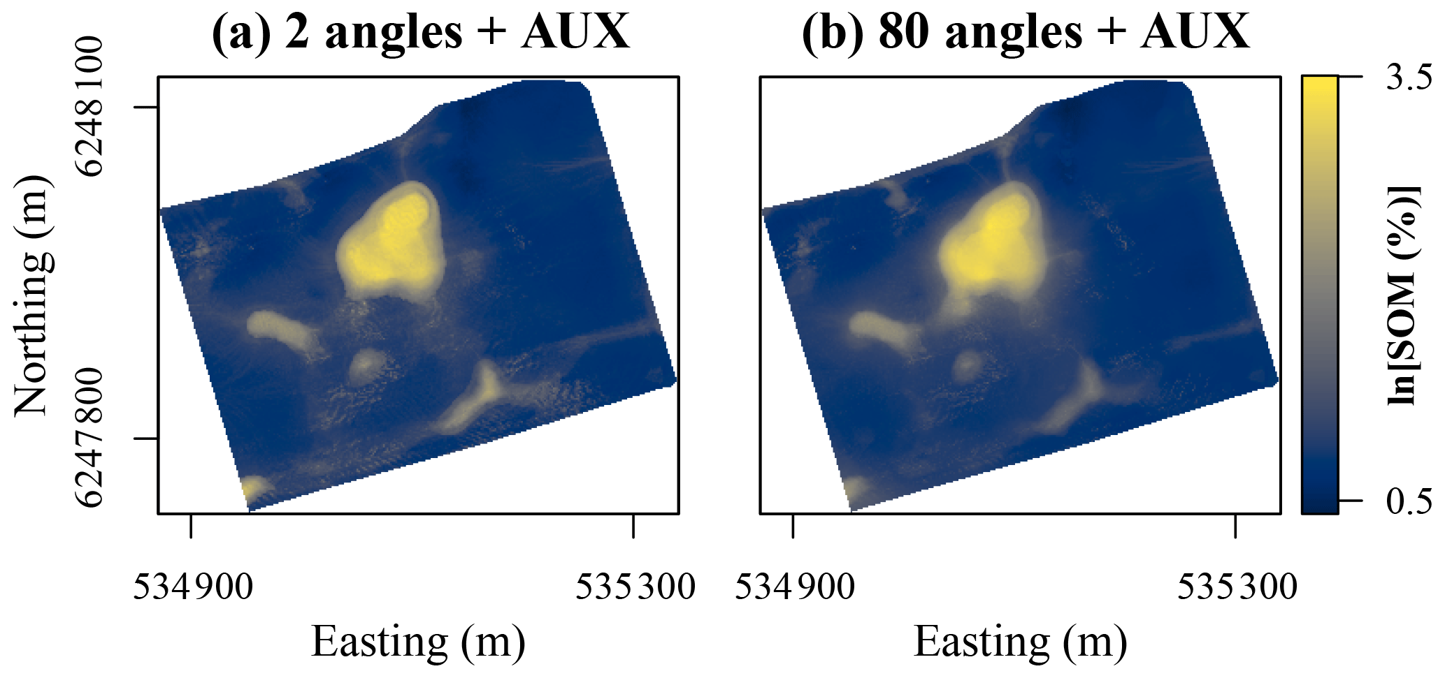
Figure 6Maps of soil organic matter (SOM) contents in the topsoil at Vindum predicted using random forest models trained using auxiliary data in conjunction with coordinate rasters at (a) 2 and (b) 80 different angles as covariates. Easting and northing for UTM zone 32N (ETRS89).
With auxiliary data, the effect of increasing the number of coordinate rasters was less clearly visible for the Vindum dataset (Fig. 6). Even with only two coordinate rasters, the predictions had no orthogonal artifacts. However, they contained noisy patterns and sharp boundaries in some areas. This is most likely an artifact from the auxiliary data. For example, using a high-resolution DEM may have created noise in the predictions. However, with coordinate rasters at 80 different angles, the spatial pattern of the predicted SOM contents became substantially smoother, with a reduction in both noise and sharp boundaries. Furthermore, some areas with moderately high SOM contents became more clearly visible and coherent, for example, in the area approximately one-third of the way from the western to the northern corner of study area. The predicted patterns with a higher number of coordinate rasters were therefore not only more accurate but also more realistic.

Figure 7Violin plots showing accuracies of soil organic matter predictions on the Vindum dataset with kriging, and random forest models trained using either auxiliary data (AUX), Euclidean distance fields (EDFs), distances to observations (RFsp), oblique geographic coordinates (OGCs), or EDFs, RFsp, or OGCs in conjunction with AUX. The figure shows Pearson's R2, root mean square error (RMSE) and Lin's concordance obtained from 100 repeated splits (75 % training dataset; 25 % test dataset).
3.1.2 Additional datasets
For the three additional datasets, the effect of increasing the number of coordinate rasters without auxiliary data was generally the same as for the Vindum dataset. In all three cases, there was relatively little, if any, increase in accuracy after an initially very steep increase. For the meuse dataset, the optimal number of coordinate rasters was six or eight, depending on the accuracy metric (Fig. A1 in the Appendix). For the eberg dataset, the optimal number was 91, but there was only limited improvement in accuracy with more than five coordinate rasters (Fig. A3). For the Swiss rainfall dataset, the optimal number of coordinate rasters was 33 or 50, depending on the accuracy metric (Fig. A5).
As for the Vindum dataset, the optimal number of coordinate rasters was generally larger in combination with auxiliary data than without auxiliary data. For the meuse dataset, the optimal number of coordinate rasters in combination with auxiliary data was 11 or 13, depending on the accuracy metric. For the eberg dataset, the optimal number of coordinate rasters in combination with auxiliary data was 22. However, unlike the results for the Vindum dataset, accuracies for these two datasets gradually decreased when the number of coordinate rasters was larger than the optimal value.
In summary, the combination of OGCs with auxiliary data generally increased the optimal number of coordinate rasters. Furthermore, in some cases, accuracy deteriorates when the number of coordinate rasters surpasses an optimal value, while in other cases it reaches a plateau. The decrease in accuracy past the optimum may be due to the correlation between the coordinate rasters. Coordinates x and y are perfectly uncorrelated, but the coordinate rasters become increasingly correlated as their number increases. The optimal value may therefore be a trade-off between the increased ability of the model to account for spatial trends and the adverse effect of increasingly correlated covariates. It is therefore likely that it depends on the complexity of the spatial distribution of the target variable and the number of observations.
With OGCs in combination with auxiliary data, the process-based covariates in the auxiliary data most likely help to reduce the effect of correlation between the coordinate rasters. Furthermore, in this case, the number of coordinate rasters also affects the relative weighting between the auxiliary data and the coordinate rasters. When mtry is smaller than the total number of covariates, a higher number of coordinate rasters increases the chance that a coordinate raster will be available for a split. The optimal number of coordinate rasters may therefore depend on the optimal weighting between process-based and explicitly spatial covariates. This optimal weighting may depend on the number of covariates in the auxiliary data and the strength of the relationship between the target variable and the auxiliary data.
At present, several factors could therefore explain the optimal number of coordinate rasters for each dataset with and without auxiliary data. The exact interplay between these factors is unclear, and the best option may therefore be to experiment with different numbers of coordinate rasters.
3.2 Method comparison
3.2.1 Predictive accuracy
For all four datasets, there were large overlaps in the accuracies of the methods, as accuracies varied across the 100 repeated splits (Figs. 7, A2, A4 and A6). However, an analysis on the Vindum dataset revealed that the accuracies generally correlated between the methods across the repeated splits. The mean correlation coefficient (Pearson's R) was 0.52 (0.19–0.88) for R2, 0.71 (0.65–0.71) for RMSE and 0.65 (0.41–0.89) for ccc. This shows that some holdout datasets yielded consistently high accuracies, while others yielded consistently low accuracies. Furthermore, especially for R2 and ccc, a few holdout datasets yielded much lower accuracies than the other holdout datasets, leading to long negative tails (Figs. 7, A2 and A6).
Table 1Auxiliary data variables used as covariates in the study including the name, the description, the mean value and the range. Pouladi et al. (2019) describe the derivation of the variables.
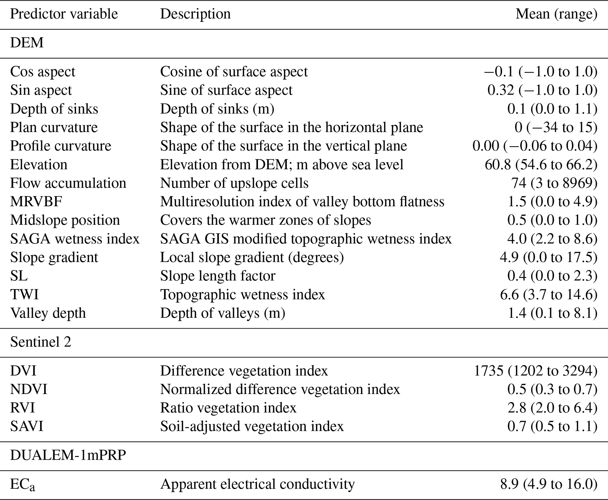
Table 2Ranks for the accuracies of the methods on the Vindum dataset calculated as Pearson's R2, RMSE and ccc, respectively. Methods for which a pairwise t test did not give a significant difference in accuracy (p>0.05) received equal ranks for the metric in question. Ranks for the methods therefore differ between the three metrics. AUX – auxiliary data; EDFs – Euclidean distance fields; OGCs – oblique geographic coordinates; and RFsp – distances between observations.
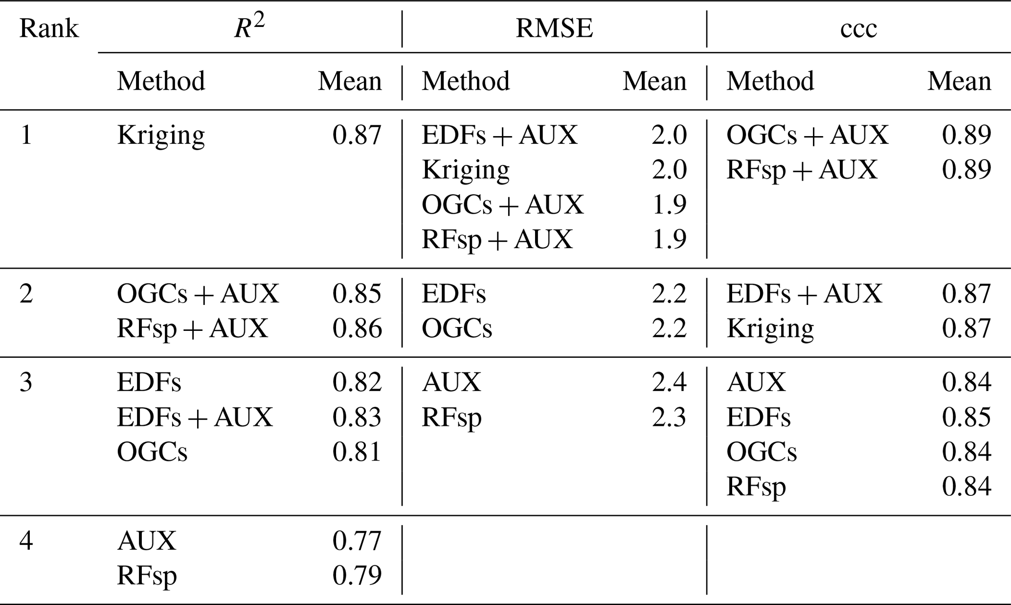
For the Vindum dataset, kriging achieved the highest rank for R2 (Table 2). For RMSE, kriging shared the highest rank with EDFs, RFsp and OGCs in combination with auxiliary data. Lastly, OGCs and RFsp in combination with auxiliary data shared the highest rank for ccc. In short, kriging, RFsp with auxiliary data and OGCs with auxiliary data all had the highest rank for two accuracy metrics out of three. We therefore regard these three methods as the most accurate methods for the Vindum dataset. Furthermore, we regard these three methods as equally accurate for this dataset, as none of them was universally more accurate than the other two methods.
Auxiliary data used on their own, and RFsp without auxiliary data, had the lowest rank for all three accuracy metrics on the Vindum dataset. Furthermore, OGCs without auxiliary data had the same rank as EDFs without auxiliary data for all three accuracy metrics.
Pouladi et al. (2019) tested several methods for predicting SOM on the Vindum dataset, including kriging and the machine-learning algorithms cubist and random forest, with and without kriged residuals. The authors found that kriging provided the most accurate predictions of SOM. The results for Vindum affirm the high accuracy of kriging predictions, but they also show that random forest models combining auxiliary data with spatial trends can achieve similar accuracies.
Table 3Ranked accuracies obtained with each method on the meuse dataset, calculated as Pearson's R2, RMSE and ccc. Methods received shared ranks if a pairwise t test revealed no statistically significant difference between their accuracies for the metric in question. Each t test used accuracies obtained with 100 repeated splits into training and test datasets. AUX – auxiliary data; EDFs – Euclidean distance fields; RFsp – distances to observations; OGCs – oblique geographic coordinates; OK – ordinary kriging; and RK – regression kriging.
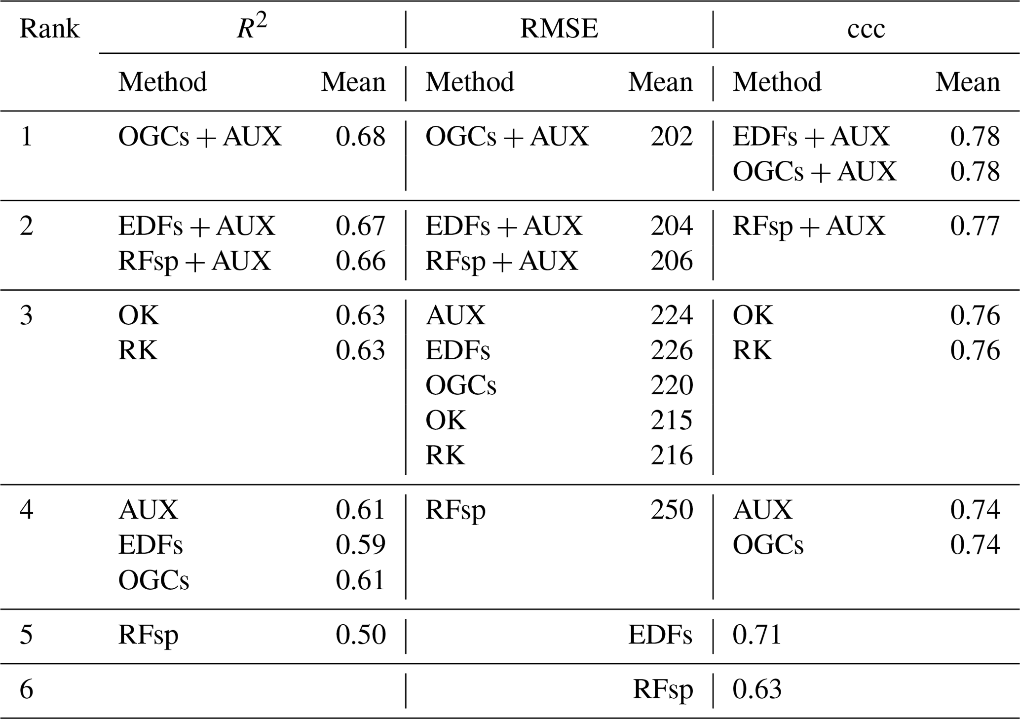
For the meuse dataset, OGCs in combination with auxiliary data achieved the highest rank for R2 and RMSE (Table 3). For ccc, OGCs in combination with auxiliary data shared the highest rank with EDFs in combination with auxiliary data. Without auxiliary data, OGCs received the third rank for RMSE and the fourth rank with R2 and ccc. OGCs without auxiliary data were generally on par with models based only on auxiliary data and with EDFs. They were less accurate than combined methods and OK (R2 and ccc). RFsp without auxiliary data was the least accurate method.
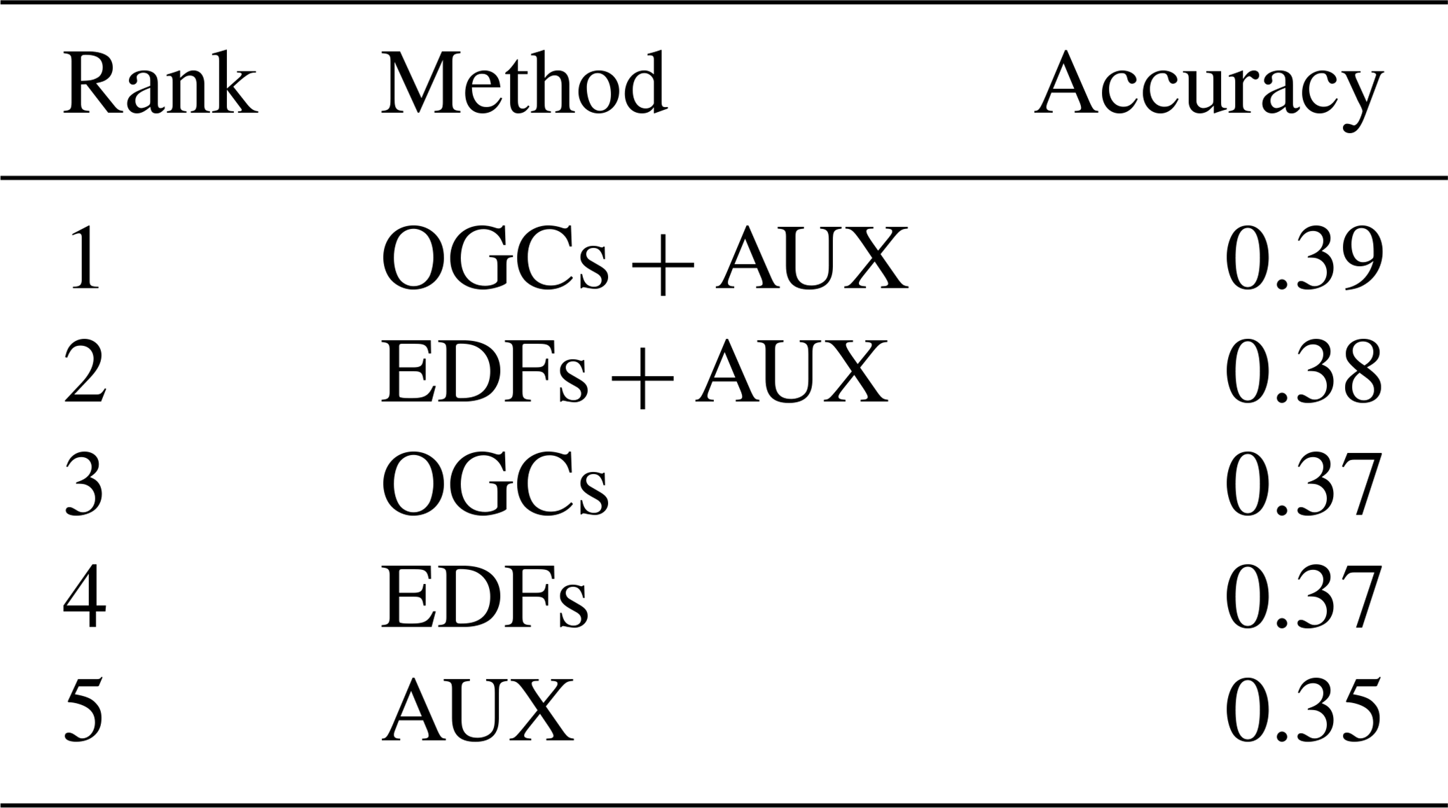
For the eberg dataset, OGCs in combination with auxiliary data were the most accurate method (Table 4). Without auxiliary data, OGCs had the third rank. They were less accurate than EDFs combined with auxiliary data but more accurate than EDFs without auxiliary data and models based only on auxiliary data. Models based only on auxiliary data yielded the lowest accuracies.
Table 4Ranks of the accuracies (percent cases correctly predicted) obtained with each method on the eberg dataset. Pairwise t tests showed that differences between the accuracies of the methods were all statistically significant (p<0.05). AUX – auxiliary data; EDFs – Euclidean distance fields; and OGCs – oblique geographic coordinates.
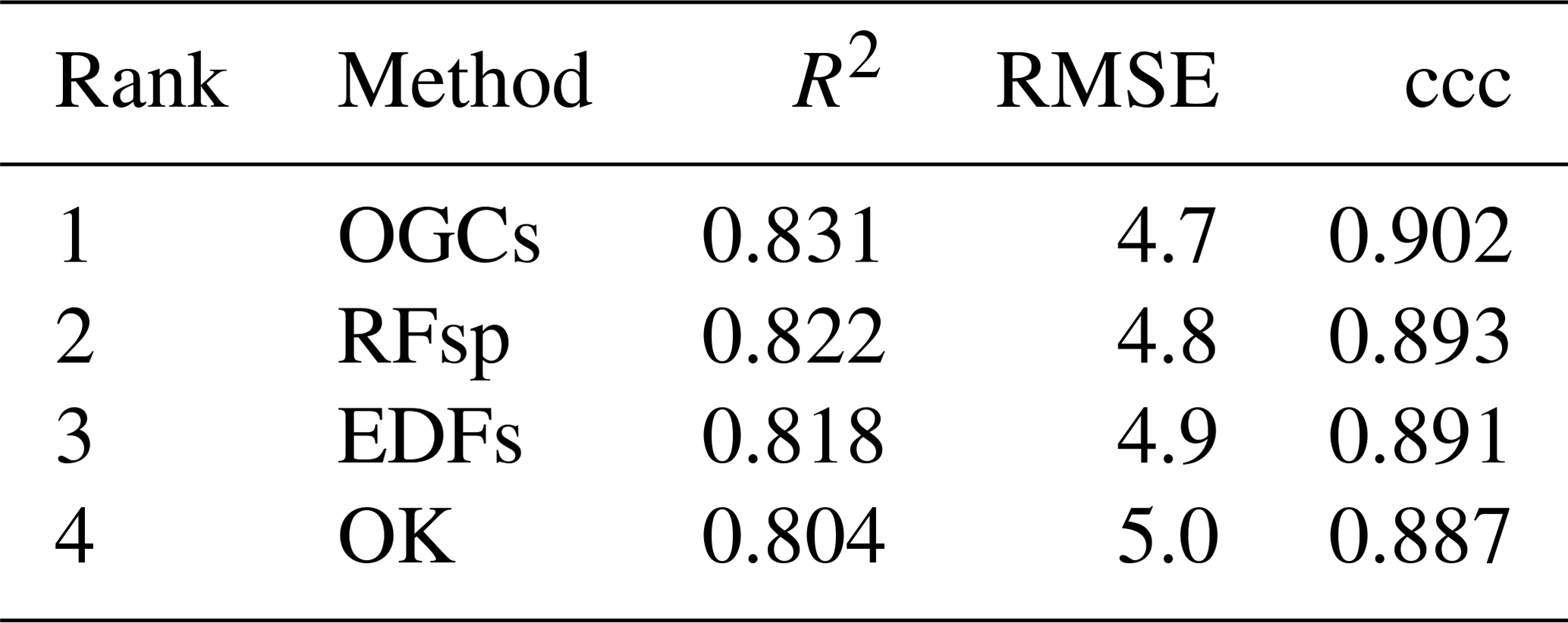
For the Swiss rainfall dataset, OGCs were the most accurate method for all three metrics (Table 5). RFsp was the second most accurate method, followed by EDFs. OK was the least accurate method.
Table 5Ranked accuracies on the Swiss rainfall dataset for each method. Pairwise t test showed statistically significant (p<0.05) differences between the methods for all three metrics. The ranks are the same for all three metrics. EDFs – Euclidean distance fields; RFsp – distances to observations; OGCs – oblique geographic coordinates; and OK – ordinary kriging.
In summary, for Vindum, meuse and eberg, OGCs combined with auxiliary data were either the most accurate method or one of the most accurate methods. Without auxiliary data, OGCs were not one of the most accurate methods for these datasets. However, for the Swiss rainfall dataset, OGCs were the most accurate method, even though we used no auxiliary data.
It is important to consider that in most cases all methods yielded acceptable accuracies. Although the differences between the accuracies of the methods were in many cases statistically significant, they were generally small. However, the results show that OGCs compare well with other methods for integrating spatial trends in machine-learning models.
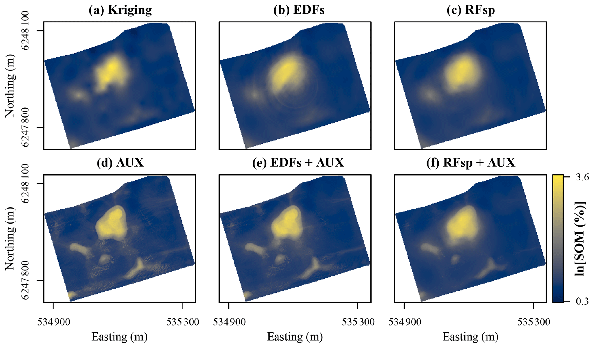
Figure 8Prediction of soil organic matter (SOM) contents for the topsoil at Vindum using (a) kriging, or random forest models trained with (b) Euclidean distance fields (EDFs), (c) distances to observations (RFsp), (d) auxiliary data (AUX), (e) EDFs in conjunction with AUX, or (f) RFsp in conjunction with AUX. Easting and northing for UTM zone 32N (ETRS89).
3.2.2 Maps
For the Vindum dataset, kriging produced a smooth prediction surface, which is very common for this method (Fig. 8a). The prediction surface with EDFs was mostly smooth, but it also contained a distinct “rings in the water” artifact caused by the raster with the distance to the middle of the study area (Fig. 8b). The prediction surface with RFsp was smoother than the prediction surface produced by kriging (Fig. 8c). The predictions with only auxiliary data were very similar to the predictions made with x and y coordinates in combination with auxiliary data (compare Figs. 8c and 6a). In combination with auxiliary data, both EDFs and RFsp produced smoothing effects similar to the effect seen with OGCs in combination with auxiliary data (compare Figs. 8e–f to 6b). However, for EDFs the smoothing was less visible than with OGCs and for RFsp it was more visible than with OGCs.
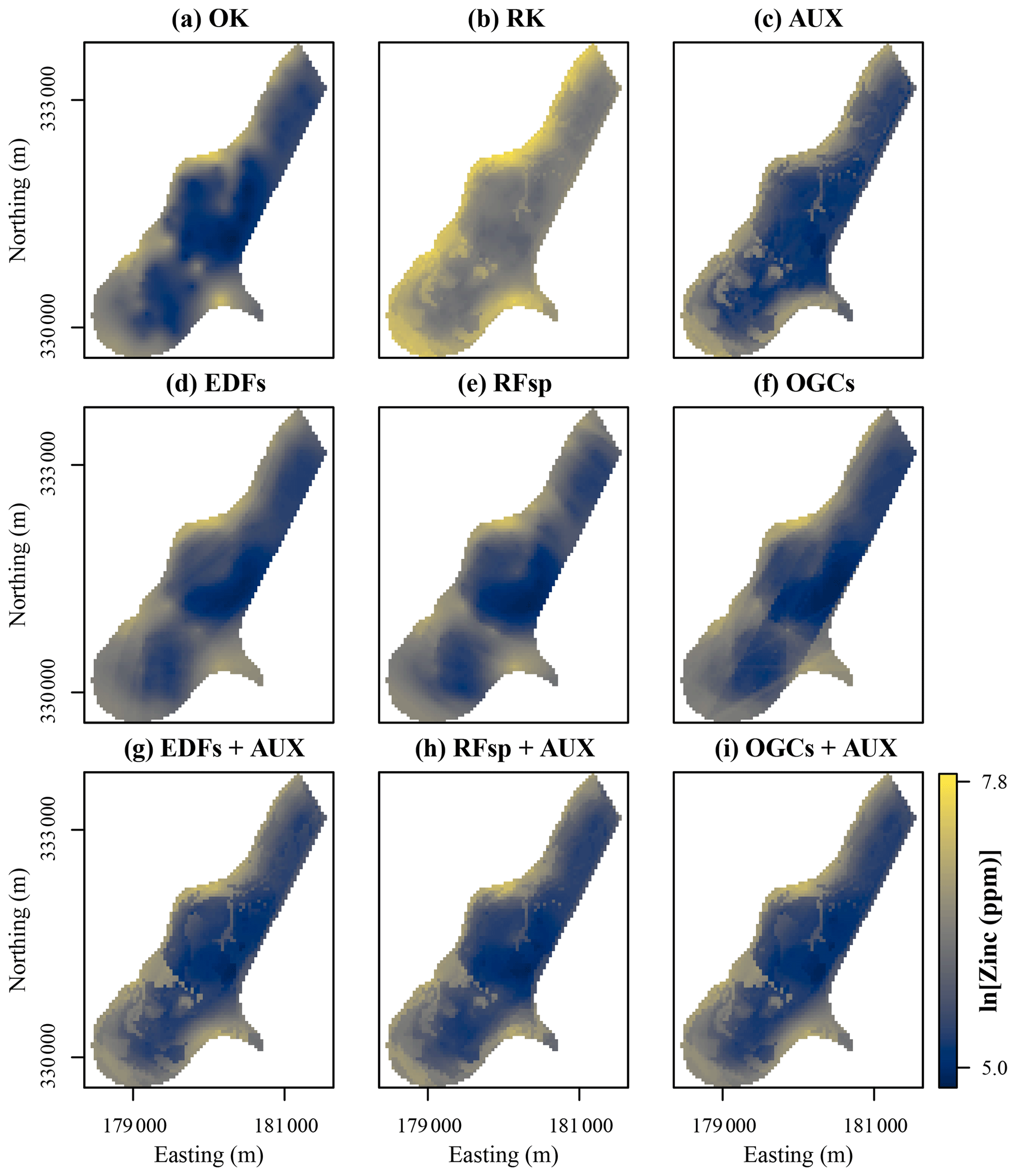
Figure 9Zinc contents predicted with each method for the meuse dataset. Easting and northing are Rijksdriehoek (RDH; Netherlands topographical map) coordinates. (a) Ordinary kriging (OK), (b) regression kriging (RK), (c) auxiliary data (AUX), (d) Euclidean distance fields (EDFs), (e) distances to observations (RFsp), (f) oblique geographic coordinates (OGCs), (g) EDFs combined with AUX, (h) RFsp combined with AUX, and (i) OGCs combined with AUX.
For the meuse dataset, OK, EDFs and RFsp produced smooth prediction surfaces (Fig. 9). However, OGCs without auxiliary data produced a prediction surface with several abrupt, angular artifacts. The accuracy of OGCs without auxiliary data was on par with some of the other methods, but the maps revealed that the predictions were not realistic. Predictions with the combined methods (RK, EDFs + AUX, RFsp + AUX and OGCs + AUX) were mostly similar to predictions with only auxiliary data. However, in some places these methods smoothed out the spatial patterns produced with only auxiliary data (for example, in the northern part of the study area), and in other places they made them more distinct (for example, southwest of the middle of the study area). In this regard, the results are similar to the results from Vindum.
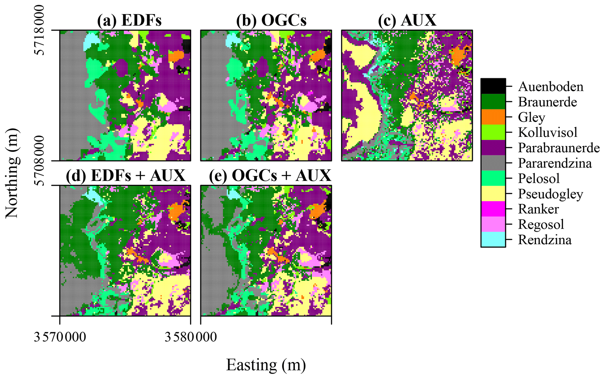
Figure 10Soil types predicted with each method for the eberg dataset. Easting and northing are coordinates according to DHDN/Gauss–Krueger zone 3 (German coordinate system). (a) Euclidean distance fields (EDFs), (b) oblique geographic coordinates (OGCs), (c) auxiliary data (AUX), (d) EDFs combined with AUX, and (e) OGCs combined with AUX.
For the eberg dataset, predictions based only on auxiliary data showed a very noisy spatial pattern with many soil types occupying small, incoherent areas (Fig. 10c). The spatial patterns produced with OGCs and especially EDFs were much smoother and contained several large, rounded areas with little internal variation in soil types (Fig. 10a and b). The predictions obtained with the combined methods were similar to the spatial pattern obtained with only auxiliary data. However, they were much smoother as the soil types occupied mostly coherent areas. The effect for predictions of soil types therefore appears similar to the effect for numeric variables seen for Vindum and meuse.
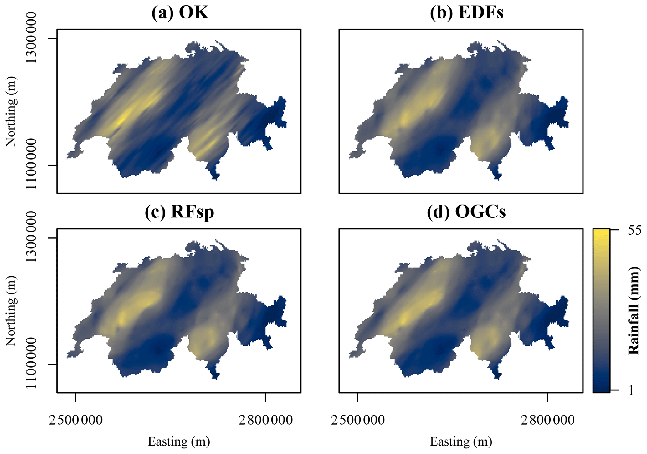
Figure 11Maps of rainfall on 8 May 1986 in Switzerland predicted with each method. Northing and easting are coordinates according to the Swiss coordinate system LV95. (a) Ordinary kriging (OK), (b) Euclidean distance fields (EDFs), (c) distances to observations (RFsp), and (d) oblique geographic coordinates (OGCs).
For the Swiss rainfall dataset, OK produced a smooth, highly anisotropic prediction surface (Fig. 11a). The prediction surfaces of EDFs, RFsp and OGCs also showed anisotropy, but they were generally smoother and more rounded. For example, with OK, some individual observations showed an effect on the prediction surface as elongated spots in the direction of the anisotropy. With the other three methods, a few individual observations showed an effect in the prediction surface, but their effects are more rounded and less distinct. The predictions with EDFs, RFsp and OGCs therefore appear more general than the OK predictions. Moreover, the prediction surfaces of EDFs, RFsp and OGCs appear very similar.
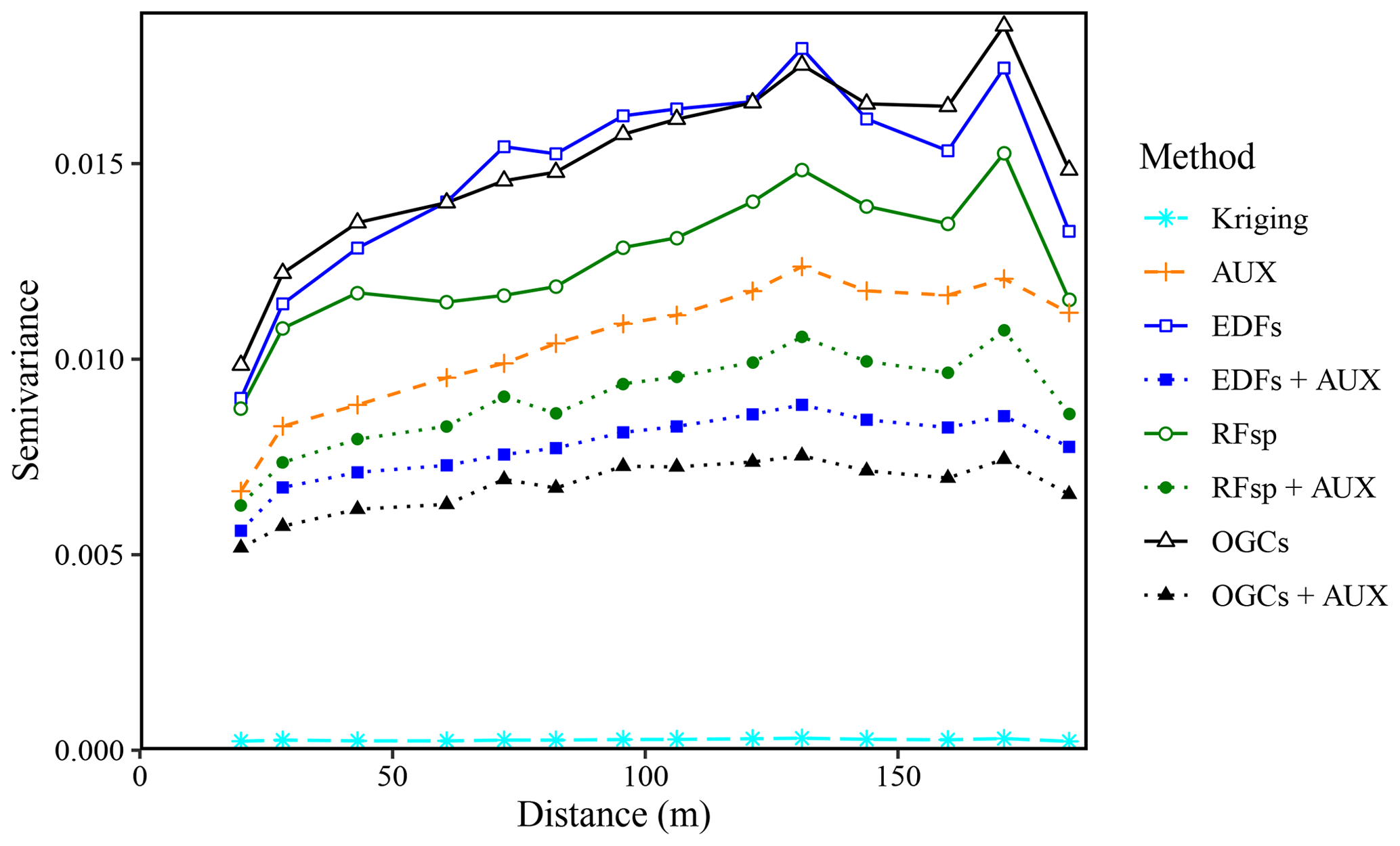
Figure 12Experimental variograms for the residuals of the SOM predictions made with each method for the Vindum dataset. The variograms use residuals from natural logarithmic-transformed SOM measurements and predictions. AUX – auxiliary data; EDFs – Euclidean distance fields; RFsp – spatial random forest; and OGCs – oblique geographic coordinates.
3.2.3 Residuals
For the Vindum dataset, the residuals of the SOM predictions had some degree of spatial dependence for all methods except kriging (Fig. 12). This finding contrasts with Hengl et al. (2018), who found that there was no spatial trend in the residuals of predictions with RFsp. EDFs, RFsp and OGCs used without auxiliary data had the most spatially dependent residuals. However, the residuals of the combined methods (EDFs + AUX, RFsp + AUX and OGCs + AUX) had less spatial dependence than the residuals of models based only on auxiliary data. OGCs + AUX was the machine-learning method with the least spatially dependent residuals, although the residuals still had more spatial dependence than kriging residuals.
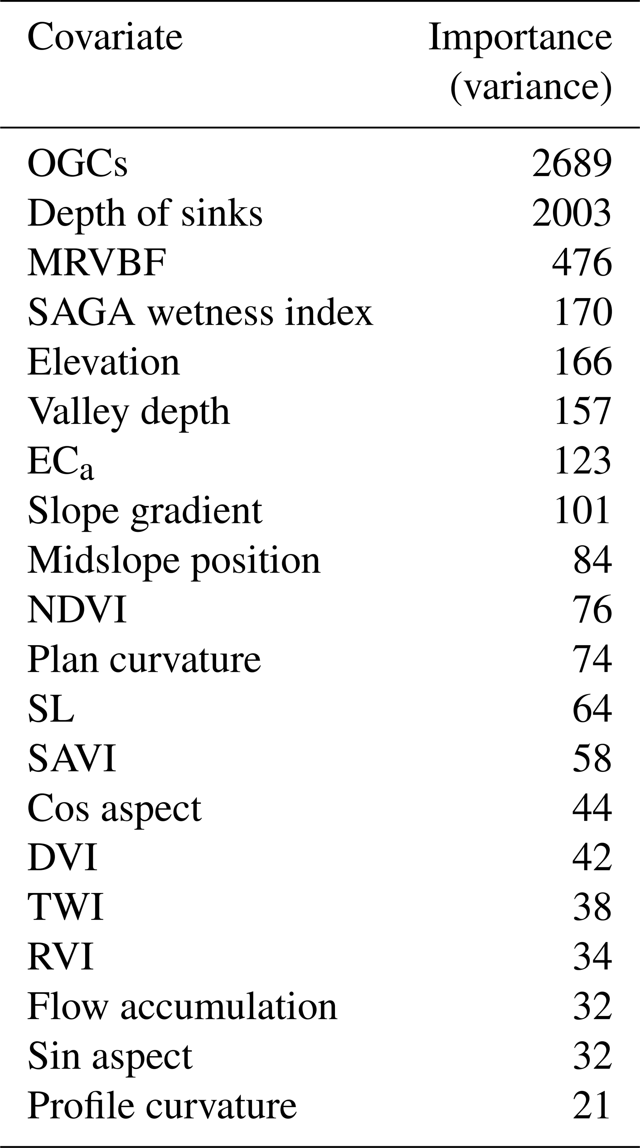
Table 6Covariate importance of the model using OGCs in combination with auxiliary data for Vindum. The importance of OGCs represents the sum of the importance of the coordinate rasters at 80 different angles.
3.3 Covariate importance
For the Vindum dataset, the most important covariate from the auxiliary data was the depth of sinks (Table 6). The most likely reason for its high importance is the presence of a large sink with very high SOM contents northwest of the middle of this study area (Fig. 1). As sinks trap surface runoff, they often have wet conditions, which give rise to peat accumulation.
When used in combination with the auxiliary data, the importance of the individual coordinate rasters varied from 0.6 % to 3.1 % of the importance of the depth of sinks, with mean value of 1.7 %. The most important coordinate raster had θ=0.48π (close to a north–south axis) and was the 12th most important covariate. The sum of the importance of the coordinate rasters was equal to 134.3 % of the importance of the depth of sinks (Table 6). Therefore, with coordinate rasters at 80 different angles, the effect of the individual rasters on the predictions was subtle, but their combined effect was strong.
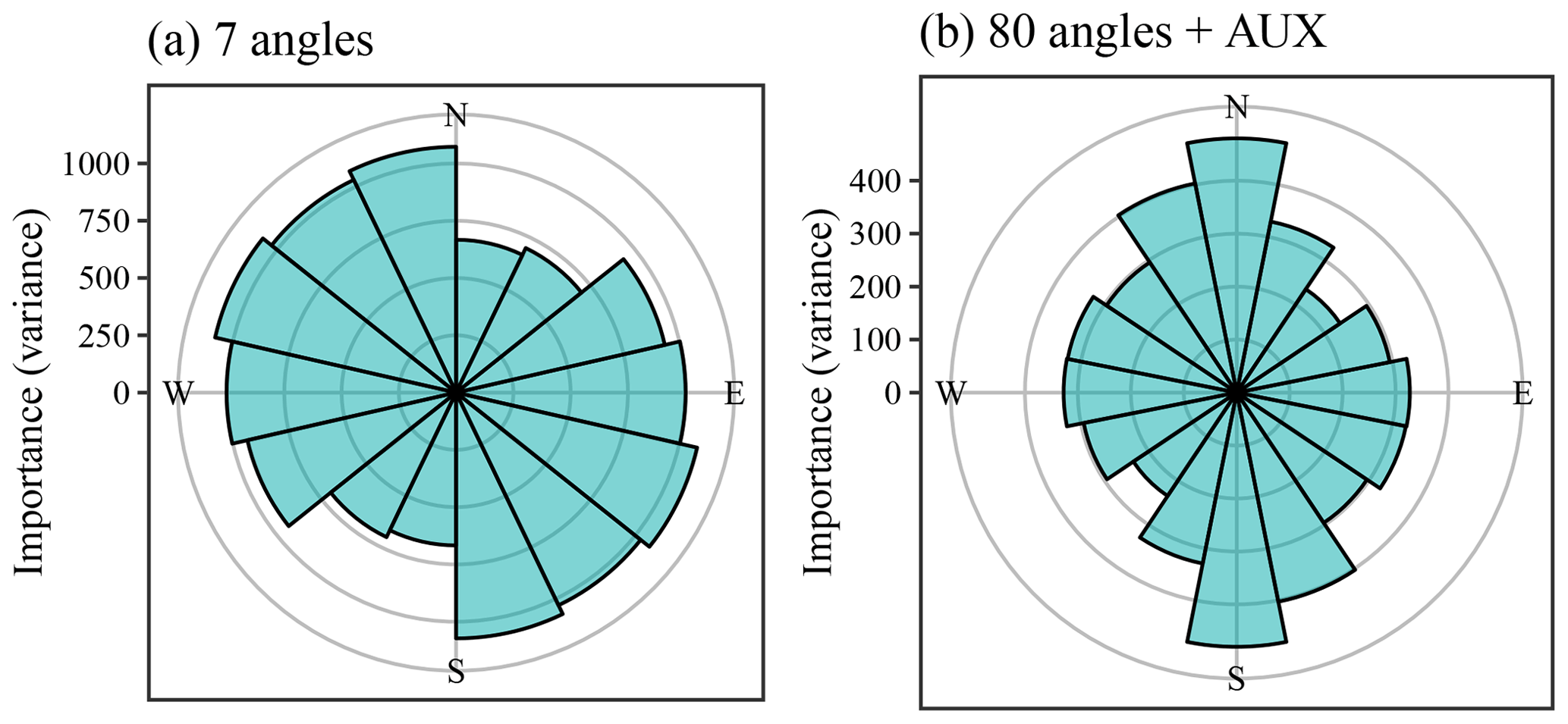
Figure 13Covariate importance of the coordinate rasters at various angles for Vindum. (a) Importance of coordinate rasters at seven different angles. (b) Importance of coordinate rasters at 80 different angles used with auxiliary data (importance of auxiliary data not shown). The sizes of the bars show the importance of the coordinate rasters at a given angle. Bars in (b) show the sum of the importance of coordinate rasters aggregated into 0.125π intervals.
Figure 13 shows the importance of the coordinate rasters relative to θ in a way that is similar to a wind rose. The plots repeat the bars for θ≥π, as the importance of a given angle is directionless. For example, the importance of θ=0 (east) is equal to the importance of θ=π (west).
Without auxiliary data, the most important coordinate rasters had a general northwestern to southeastern angle (Fig. 13). On the other hand, the coordinate rasters with angles between a north–south and a northeast–southwest axis had low importance. The most likely reason for this pattern is the location of the sink with very high SOM contents to the northwest of the middle of this study area. This creates a large difference in the SOM contents of the northwestern and southeastern parts of the study area, giving large importance to covariates that can explain this difference. Additionally, the northwestern side of the sink has a very steep slope, creating a steep gradient in SOM contents in this direction. A stable variogram showed anisotropy along a north–northeast to south–southwest axis (θ=0.34π), with a major range of 136 m and a minor range of 118 m. The direction of the anisotropy therefore coincided with the direction of the least important coordinate rasters.
On the other hand, with OGCs in combination with auxiliary data, the most important coordinate rasters had tilt angles close to a north–south axis (θ=0.5π). At the same time, the least important coordinate rasters had tilt angles close to a northeast–southwest axis (θ=0.25π). The residuals from the predictions with only auxiliary data also displayed a degree of anisotropy. A stable variogram showed anisotropy along a northeast to southwest axis (θ=0.21π), with a major range of 52 m and a minor range of 38 m. Again, the angle of the anisotropy coincided with the angle of the least important coordinate rasters. The spatial pattern of the residuals therefore differed from the spatial pattern of the SOM contents in the Vindum study area. Apparently, there are unaccounted for processes decreasing the spatial variation along a northeast–southwest axis relative to other angles.
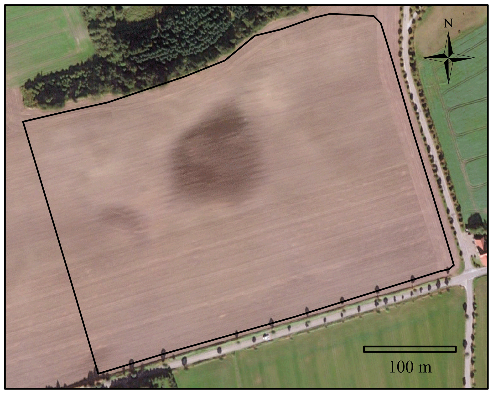
Figure 14Orthophoto of the study area from 27 September 2016 (Esri, 2019). Sources: Esri, DigitalGlobe, Earthstar Geographics, CNES/Airbus DS, GeoEye, USDA FSA, USGS, Aerogrid, IGN, IGP, and the GIS User Community.
A possible cause of the anisotropy in the residuals may be the plowing direction. The main plowing direction in the Vindum study area is along an east–northeast to west–southwest axis (θ=0.18π). This angle is nearly parallel to the angle of the least important coordinate rasters (Fig. 14). The plowing direction, combined with the topography, has a large impact on soil movement, as plowing displaces soil both along and across its direction (Lindstrom et al., 1990; De Alba, 2003; Heckrath et al., 2006). Most of the study area has the same plowing direction, irrespective of the topography, resulting in up-, down- and cross-slope plowing in various parts of the field. This creates in a complex pattern of soil redistribution, which likely affects the SOM contents of the topsoil. As downslope soil movement is strongest in the plowing direction, variation in soil properties parallel to this direction is likely to be smaller than the variation perpendicular to the plowing direction. This corresponds to the low importance of coordinate rasters with angles close to the plowing direction. However, none of the auxiliary data accounted for the plowing direction. This indicates that OGCs can add information on the most likely processes affecting soil properties in an area.
3.4 Choice of method
At Vindum, the three most accurate methods were kriging, RFsp with auxiliary data and OGCs with auxiliary data. For meuse, OGCs and EDFs combined with auxiliary data were most accurate and for eberg, OGCs combined with auxiliary data were most accurate. For the Swiss rainfall dataset, OGCs were the most accurate method.
Although kriging was in most cases less accurate than other methods, some soil mappers would probably still choose it for mapping soil properties due to its computational efficiency and conceptual simplicity. However, aside from accuracy, an advantage of methods based on machine learning lies in the fact that they provide larger amounts of information than geostatistical models. Kriging in itself does not provide information on the processes that control spatial variation in soil properties, but machine-learning models can include covariates related to soil processes, providing information on the processes that are most likely to affect the spatial distribution of a soil property.
With spatial approaches such as EDFs, RFsp and OGCs, researchers can incorporate feature space and geographic space in a machine-learning model. Of the previously used approaches, OGCs are most similar to EDFs, as they used the x and y coordinates, and the distances to the corners of the study area resemble the coordinates. On the other hand, RFsp is more similar to geostatistical models, as it relies on distances between observations. However, this similarity comes at the cost of calculating a large number of distance rasters.
One advantage of using spatially explicit covariates (EDFs, RFsp or OGCs) is that researchers can interpret local and spatial effects at once. In this regard, OGCs have an advantage over EDFs and RFsp, as it is clear what the coordinate rasters represent. It is less clear how researchers should interpret distances to the corners of the study area or the distance to a specific observation. We have also shown that it is straightforward to illustrate covariate importance of OGCs.
Furthermore, an advantage of OGCs relative to RFsp is that OGCs required fewer covariates to achieve the same accuracy. In fact, without auxiliary data, OGCs achieved a higher accuracy with a smaller number of covariates for the datasets of Vindum, meuse and Swiss rainfall. This demonstrates a clear advantage of OGCs, as it is possible to adjust the number of coordinate rasters. EDFs and RFsp do not presently have similar options.
We will stress that, as a rule, soil mappers should not use machine-learning models relying only on spatial trends, as EDFs, RFsp and OGCs all yielded lower accuracies without auxiliary data for the soil datasets (Vindum, meuse and eberg). Moreover, surprisingly, these methods had the most spatially autocorrelated residuals for the Vindum dataset, although they relied exclusively on spatial trends. The results therefore suggest that soil mappers should primarily use these methods in combination with auxiliary data and not on their own. If no auxiliary data are available, kriging is likely to be a better option. However, results from the Swiss rainfall dataset show that, for other spatial problems, auxiliary data may be unnecessary.
We have shown in this study that the use of oblique geographic coordinates (OGCs) is a reliable method for integrating auxiliary data with spatial trends for modeling and mapping soil properties. In most cases, the method eliminated the orthogonal artifacts that arise from the use of x and y coordinates and achieved higher accuracies than maps created with only two coordinate rasters. However, for meuse, without auxiliary data, OGCs still produced abrupt angular artifacts in the final map. Soil mappers should therefore combine OGCs with auxiliary data, as this gives higher accuracies and spatial patterns with a higher degree of realism.
OGCs are more interpretable than previous similar approaches, and more flexible, as it is possible to adjust the number of coordinate rasters. This should allow soil mappers to find a good compromise between accuracy and computational efficiency for mapping soil properties, as the optimal number of coordinate rasters may vary depending on the study area and the soil property in question.
At this point, we have only tested the method for three soil datasets and one meteorological dataset. It will therefore be highly relevant to test the method for other soil properties and areas. It will especially be relevant to test the method in larger, less densely sampled areas. Previous studies have shown that machine learning is likely to provide higher accuracies in such areas (Zhang et al., 2008; Greve et al., 2010; Keskin et al., 2019), and it will be relevant to test if this is also the case for oblique geographic coordinates. Results from the Vindum and the Swiss rainfall datasets also suggest that the method can be useful for mapping variables with anisotropic spatial distributions, and it will therefore be relevant to test it on datasets with a high degree of anisotropy. Lastly, one should note that we carried out this study for relatively small areas using “flat” coordinate systems. Using OGCs for larger areas and other coordinate systems may require alterations to the method.
We call upon researchers within digital soil mapping to aid us in testing oblique geographic coordinates as covariates for additional datasets, and we have therefore made the function for generating oblique geographic coordinates available as an R package. Moreover, to allow other researchers to test methods on the Vindum dataset, we have made it available and part of the same package.
A1 Methods
A1.1 meuse
We mapped zinc contents for the meuse dataset (155 points). The meuse dataset contains covariates including the flooding frequency and the distance to the river. We added two covariates in the form of a digital elevation model (DEM, https://www.ahn.nl/, last access: 9 July 2020) and surface water occurrence (Pekel et al., 2016). We converted the categorical raster of flooding frequency to indicator variables and transformed all the covariates to principal components. This resulted in six principal components.
We tested all the methods applied to the Vindum dataset, with the addition of regression kriging (RK). We used random forest models trained on the auxiliary data for regression and then kriged the residuals using the function krige.conv from the R package geoR (Ribeiro et al., 2020). As for the Vindum dataset, we tested each method with 100 repeated splits into training (75 %) and test (25 %) data. For each split, we calculated Pearson's R2, RMSE and ccc. We carried out pairwise t test on the accuracies obtained with each method in order to assess if the differences between their accuracies were statistically significant. We also produced maps with each of the nine methods in order to compare results.
A1.2 eberg
We mapped soil types for the eberg dataset. The eberg dataset contains 3670 soil observations. We removed points outside the coverage of the covariates and points without a soil type classification. Furthermore, we removed the soil types “Moor” and “HMoor”, as only one observation was available for each soil type. This reduced the dataset to 2552 observations.
The eberg dataset contains covariates including the parent material, a DEM, the SAGA GIS topographic wetness index and the thermal infrared reflectance from satellite imagery. We converted the parent material classes to indicators and converted all covariates to principal components. This resulted in 11 principal components.
The dataset is highly clustered, which is likely to affect accuracy assessments, as some areas have much higher point densities than others. To counter this effect, we organized the data in 100 groups using k means clustering on their coordinates. We then produced 100 splits into training and test data based on these groups. In each split, the training data contained observations from 75 groups, and the test data contained observations from the remaining 25 groups.
As we aimed to predict a categorical variable, we did not use kriging. Furthermore, due to the large size of the dataset, we did not use RFsp, as this would require us to produce more than 2000 raster layers with buffer distances. Hengl et al. (2018) avoided this by calculating only buffer distances to each soil type. However, we did not choose this solution as it would create problems for accuracy assessment. If a raster layer contains distances to test observations and training observations, the result would be circular logic, invalidating the accuracy assessment. Buffer distances based only on the training data would be less problematic. However, as we used 100 repeated splits, this was not an option.
We therefore tested only five methods for the eberg dataset, namely models based on auxiliary data (AUX), Euclidean distance fields (EDFs), OGCs, and EDFs and OGCs combined with auxiliary data.
Due to the large size of the dataset, model training was slower than for the other datasets. We therefore tuned a random forest model only once for each method and used the resulting parameterization for all 100 data splits. For each split, we calculated the accuracy on the test data as the fraction of observations correctly predicted. We carried out pairwise t tests on the accuracies obtained with each method in order to assess if the differences between their accuracies were statistically significant.
We produced maps of soil types with each of the five methods in order to compare results.
A1.3 Swiss rainfall
The Swiss rainfall dataset contains 467 rainfall observations from Switzerland from 8 May 1986. We did not use any covariates for this dataset, and we therefore tested only purely spatial methods. We tested ordinary kriging with correction for anisotropy, EDFs, RFsp and OGCs. As for the Vindum dataset, we tested each method with 100 repeated splits into training data (75 %) and test data (25 %). For each split, we calculated Pearson's R2, RMSE and ccc. We carried out pairwise t tests on the accuracies obtained with each method in order to assess if the differences between their accuracies were statistically significant. Lastly, we produced maps of rainfall with each of the four methods in order to compare results.
A2 Results
A2.1 meuse
For the meuse dataset, the accuracy of OGCs combined with auxiliary data was consistently higher than the accuracy of OGCs without auxiliary data, irrespective of the accuracy metric and the number of coordinate rasters (Fig. A1). The accuracy of OGCs initially increased quickly with the number of coordinate rasters up to an optimum, after which there was no further improvement. For OGCs + AUX, the increase in accuracy was more gradual, up to an optimum, after which the accuracy deteriorated slightly. The optimal number of coordinate rasters without auxiliary data was six for RMSE and ccc and eight for R2. With auxiliary data, the optimal number of coordinate rasters was 11 for RMSE and 13 for R2 and ccc. In the subsequent analysis, we used six coordinate rasters for OGCs without auxiliary data and 11 coordinate rasters for OGCs with auxiliary data.
For the meuse dataset, as for the Vindum dataset, the differences between the accuracies of the methods were generally small relative to the variation in accuracy between the test splits (Fig. A2). Furthermore, most methods had long tails with lower accuracies.
A2.2 eberg
For the eberg dataset, accuracy for OGCs without auxiliary data first increased sharply up to five coordinate rasters. Past this point, there was little improvement in accuracy and some numbers of coordinate rasters produced sharp, irregular drops in accuracy (Fig. A3). Combined with auxiliary data, the accuracy of OGCs increased up to 22 coordinate rasters, after which they gradually declined. Without auxiliary data, the optimal number of coordinate rasters was 91. However, the highly irregular pattern of the accuracies did not justify any number past the initial increase, and we therefore used only five coordinate rasters. For OGCs combined with auxiliary data, we used 22 coordinate rasters.
For the eberg dataset, as for the Vindum dataset, variation in accuracy between the splits into training and test data was in most cases greater than variation between the methods (Fig. A4). However, unlike the other datasets, the distributions of the accuracies were mostly symmetric.
A2.3 Swiss rainfall
For the Swiss rainfall dataset, the accuracy of OGCs generally increased with the number of coordinate rasters (Fig. A5). The increase in accuracy was steep at first, then gradual. For Pearson's R2, the optimal number of coordinate rasters was 33 and for RMSE and ccc it was 50. There was little change in accuracy past the optimal number of coordinate rasters.
As for the other datasets, variation in accuracies on the Swiss rainfall dataset was greater between the splits into training and test data than between the methods (Fig. A6). The distributions of RMSE were mostly symmetric, but the distributions of R2 and ccc had long negative tails, as some splits yielded much lower accuracies than other splits.
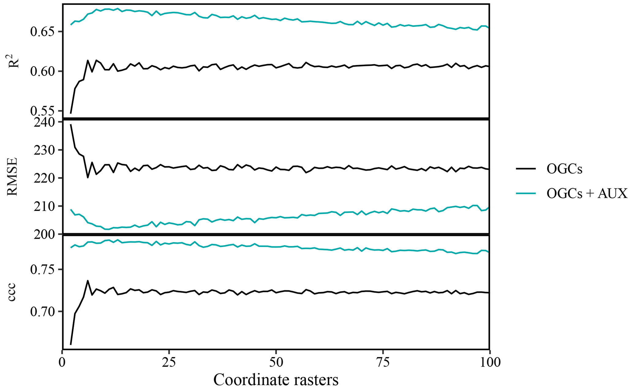
Figure A1Accuracy of predictions on the meuse dataset (zinc contents) versus the number of coordinate rasters with oblique geographic coordinates, with and without auxiliary data. The values are averages obtained with 100 splits into training and test data.

Figure A2Violin plots showing the accuracies obtained on the meuse dataset (zinc contents) with each method. The plots show values obtained with 100 splits into training and test datasets.
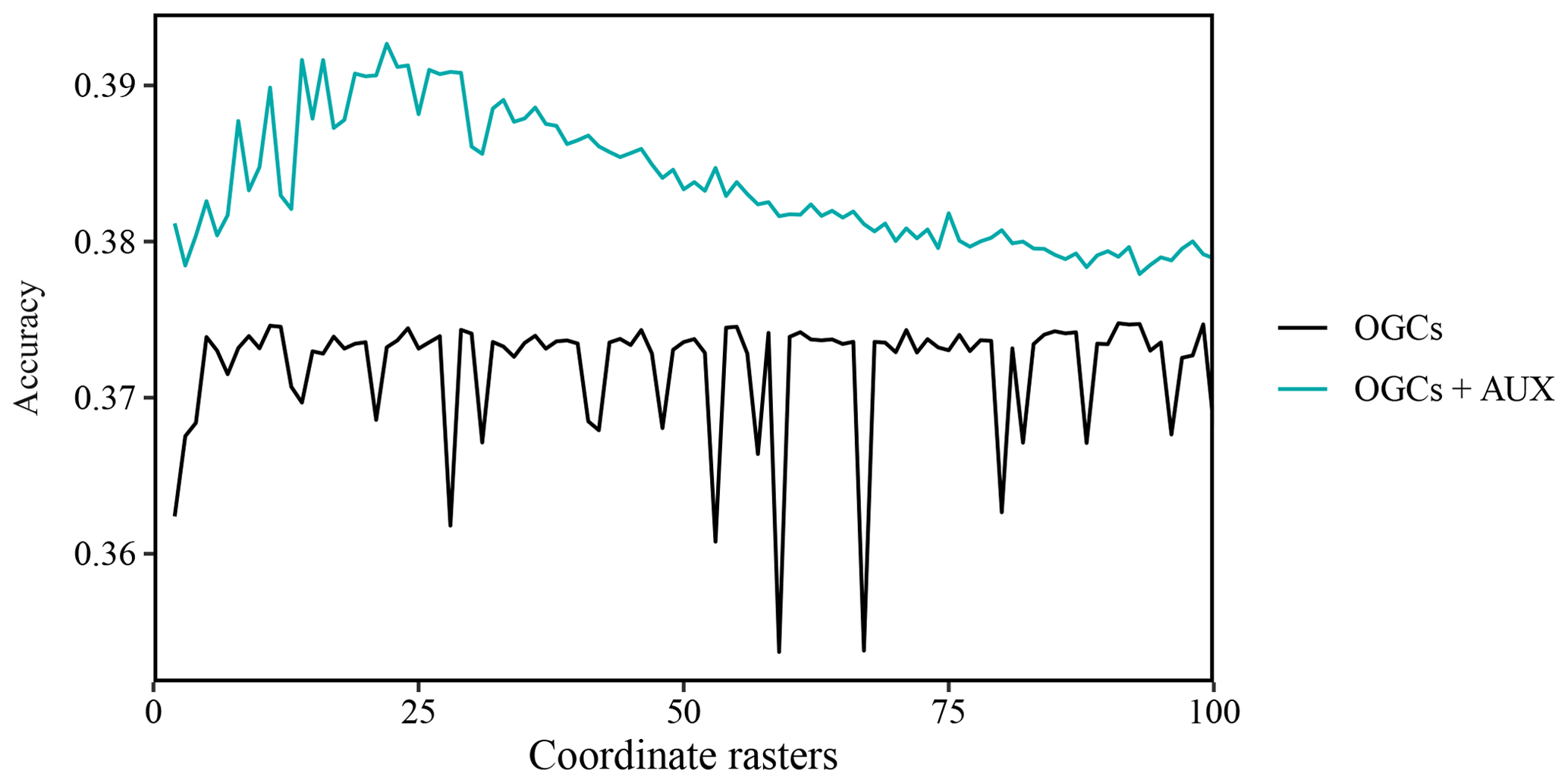
Figure A3Accuracy (percent of cases correctly predicted) of predictions on the eberg dataset versus the number of coordinate rasters with oblique geographic coordinates (OGCs), with and without auxiliary data (AUX). The values are averages obtained with 100 splits into training and test data.
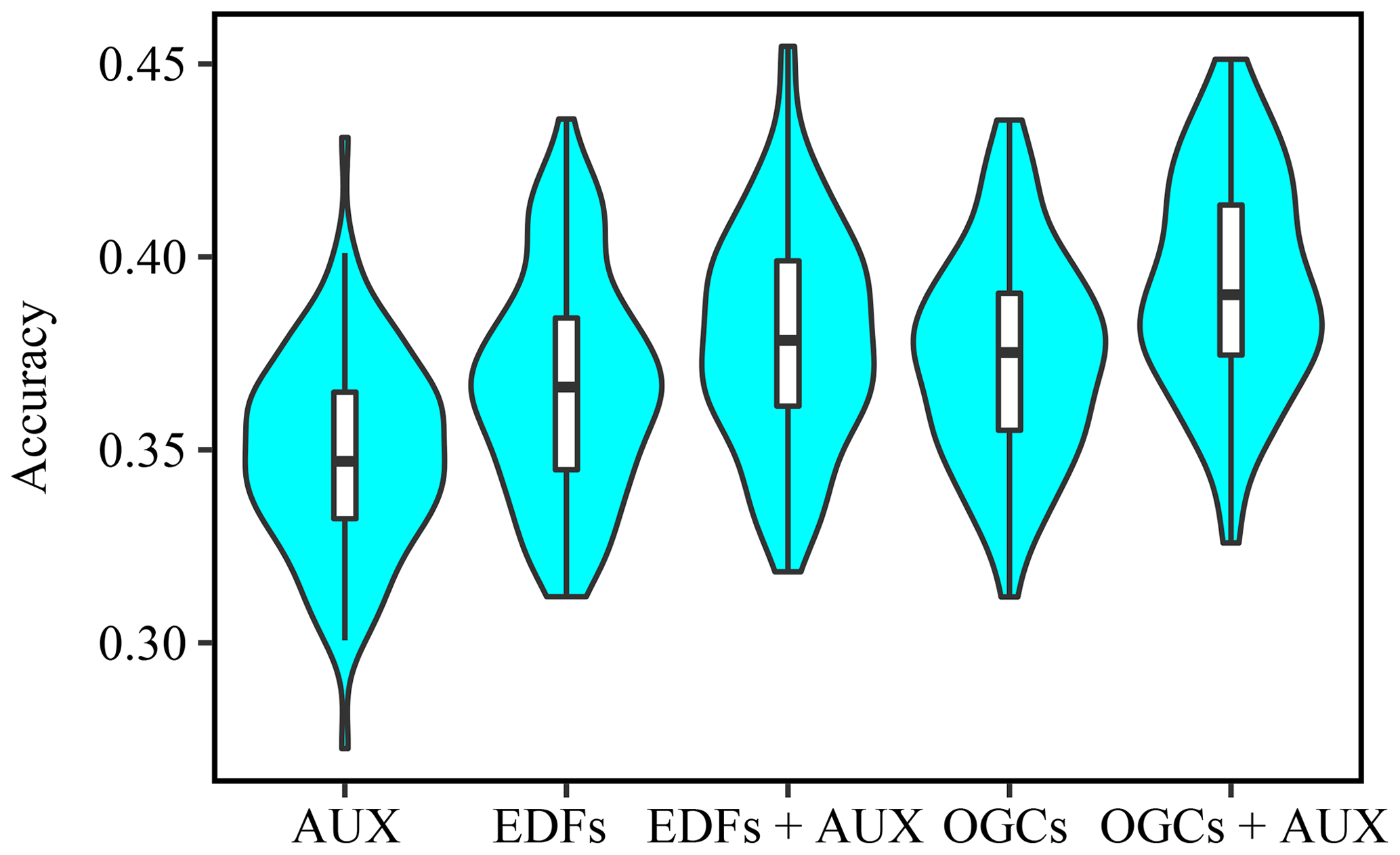
Figure A4Violin plot showing the accuracies obtained on the eberg dataset (percent correctly predicted) with each method. The plot shows values obtained with 100 splits into training and test datasets.
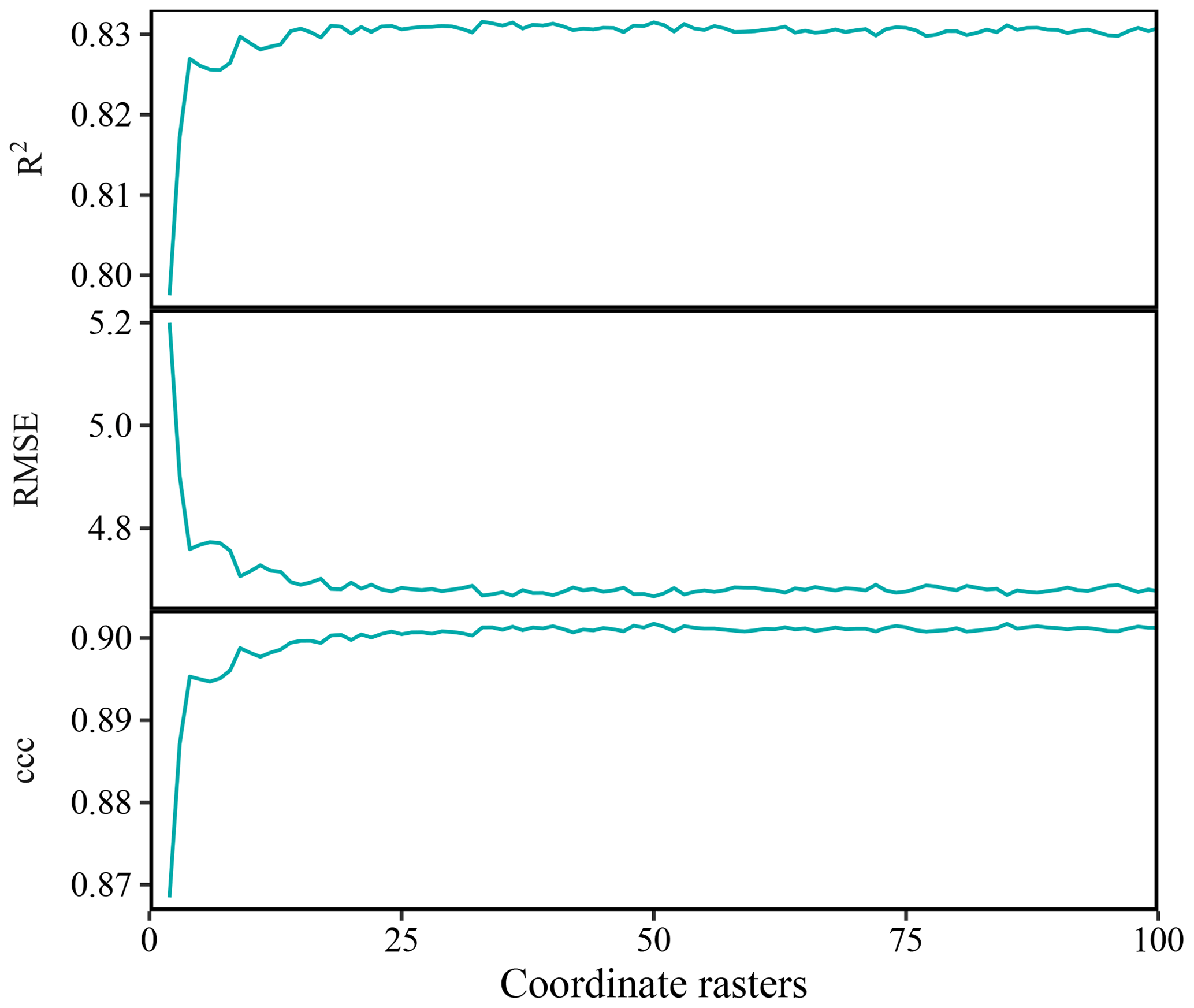
Figure A5Accuracy of predictions on the Swiss rainfall dataset versus the number of rasters with oblique geographic coordinates. The values are averages obtained with 100 splits into training and test data.
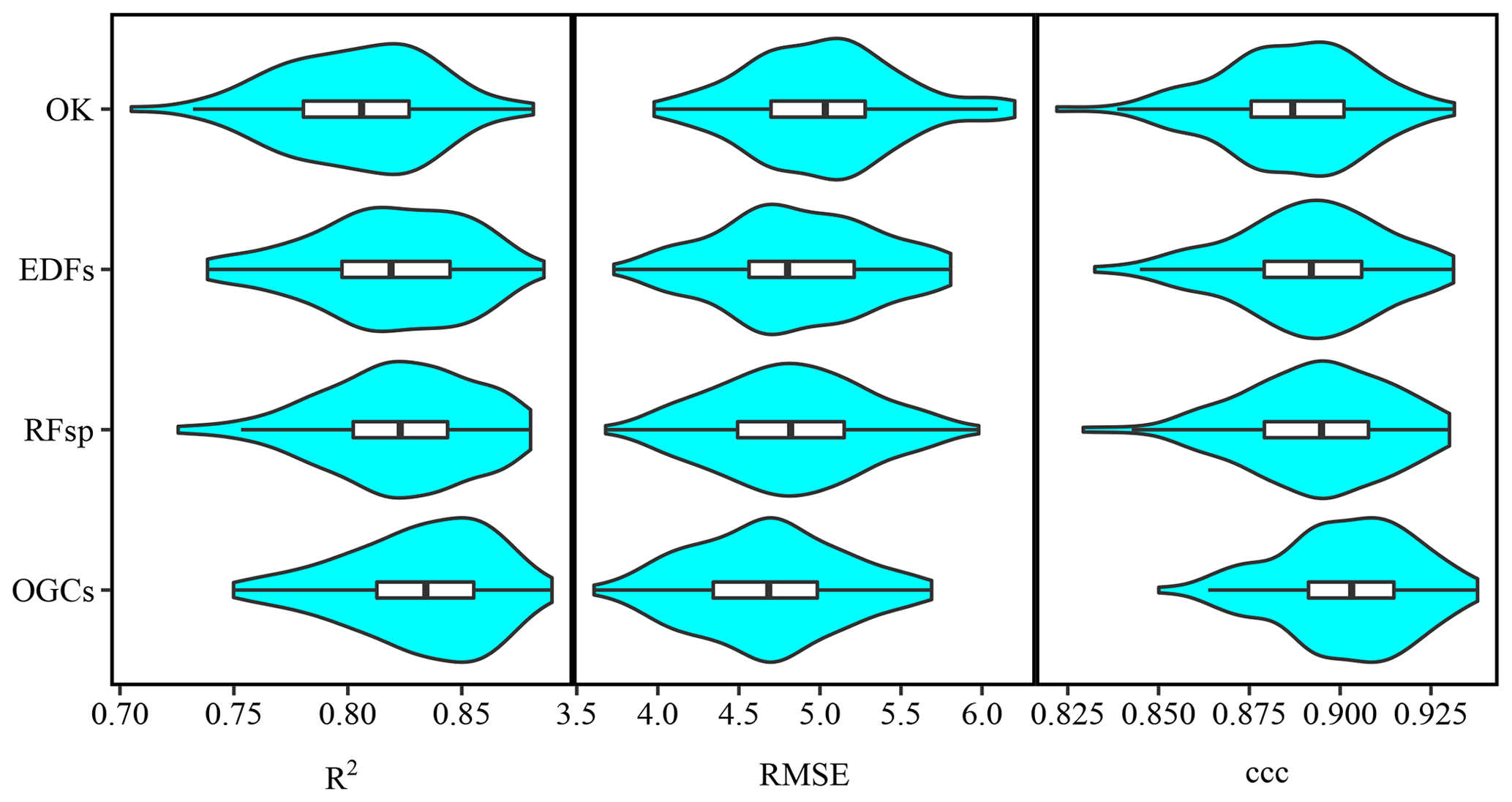
Figure A6Violin plots showing the accuracies obtained on the Swiss rainfall dataset with each method. The plots show values obtained with 100 splits into training and test datasets.
The function for generating oblique geographic coordinates is available as an R package at https://bitbucket.org/abmoeller/ogc/src/master/rPackage/OGC/ (Møller, 2019). The package also contains the SOM observations and auxiliary data from the Vindum dataset. Furthermore, we have made the R code used in this study available in a public repository at http://dx.doi.org/10.5281/zenodo.3820068 (Møller et al., 2020).
ABM and NP prepared the data. ABM carried out the analyses and prepared the paper with inputs from all coauthors.
The authors declare that they have no conflict of interest.
We are obliged to the two anonymous referees and to Alexandre Wadoux, who provided vital feedback on the paper. Their comments and advice have greatly improved the paper, and we give them our thanks.
This paper was edited by Kristof Van Oost and reviewed by two anonymous referees.
Behrens, T., Schmidt, K., Viscarra Rossel, R., Gries, P., Scholten, T., and MacMillan, R.: Spatial modelling with Euclidean distance fields and machine learning, Eur. J. Soil Sci., 69, 757–770, https://doi.org/10.1111/ejss.12687, 2018.
De Alba, S.: Simulating long-term soil redistribution generated by different patterns of mouldboard ploughing in landscapes of complex topography, Soil Tillage Res., 71, 71–86, https://doi.org/10.1016/s0167-1987(03)00042-4, 2003.
Dubois, G., Malczewski, J., and De Cort, M.: Mapping radioactivity in the environment: Spatial interpolation comparison 97, Office for Official Publications of the European Communities, 280 pp., 2003.
Esri: World Imagery, Scale not given, September 27, 2016, available at: https://www.arcgis.com/home/item.html?id=10df2279f9684e4a9f6a7f08febac2a9, last access: 19 June 2019.
Geurts, P., Ernst, D., and Wehenkel, L.: Extremely randomized trees, Mach. Learn, 63, 3–42, https://doi.org/10.1007/s10994-006-6226-1, 2006.
Greve, M. H., Greve, M. B., Kheir, R. B., Bøcher, P. K., Larsen, R., and McCloy, K.: Comparing decision tree modeling and indicator kriging for mapping the extent of organic soils in Denmark, in: Digital soil mapping: Bridging research, environmental application, and operation, edited by: Boettinger, J. L., Howell, D. W., Moore, A. C., Hartemink, A. E., and Kienast-Brown, S., Springer Netherlands, Dordrecht, 267–280 https://doi.org/10.1007/978-90-481-8863-5_22, 2010.
Heckrath, G., Halekoh, U., Djurhuus, J., and Govers, G. The effect of tillage direction on soil redistribution by mouldboard ploughing on complex slopes, Soil Tillage Res., 88, 225–241, https://doi.org/10.1016/j.still.2005.06.001, 2006.
Hengl, T., Heuvelink, G. B. M., and Stein, A. A.: generic framework for spatial prediction of soil variables based on regression-kriging, Geoderma, 120, 75–93, https://doi.org/10.1016/j.geoderma.2003.08.018, 2004.
Hengl, T., Nussbaum, M., Wright, M. N., Heuvelink, G. B., and Gräler, B.: Random forest as a generic framework for predictive modeling of spatial and spatio-temporal variables, PeerJ, 6, e5518, https://doi.org/10.7717/peerj.5518, 2018.
Hengl, T., Roudier, P., Beaudette, D., Pebesma, E., and Blaschek, M.: Package “plotKML”: Visualization of spatial and spatio-temporal objects in Google Earth, available at: https://cran.r-project.org/web/packages/plotKML/plotKML.pdf, last access: 21 April 2020.
Hiemstra, P.: Package “automap”: Automatic interpolation package, R package version 1.0-14, https://cran.r-project.org/web/packages/automap/index.html (last access: 15 August 2019), 2013.
Keskin, H., Grunwald, S., and Harris, W. G.: Digital mapping of soil carbon fractions with machine learning, Geoderma, 339, 40–58, https://doi.org/10.1016/j.geoderma.2018.12.037, 2019.
Knotters, M., Brus, D. J., and Oude Voshaar, J. H.: A comparison of kriging, co-kriging and kriging combined with regression for spatial interpolation of horizon depth with censored observations, Geoderma, 67, 227–246, https://doi.org/10.1016/0016-7061(95)00011-c, 1995.
Kuhn, M.: Building predictive models in R using the caret package, J. Stat. Softw., 28, 1–26, https://doi.org/10.18637/jss.v028.i05, 2008.
Lindstrom, M. J., Nelson, W. W., Schumacher, T. E., and Lemme, G. D.: Soil movement by tillage as affected by slope, Soil Tillage Res., 17, 255–264, https://doi.org/10.1016/0167-1987(90)90040-k, 1990.
Mitchell, T.: Decision tree learning, in: Machine Learning, McGraw Hill, New York, 52–80, 1997.
Møller, A. B.: OGC (Oblique geographic coordinates), available at: https://bitbucket.org/abmoeller/ogc/src/master/rPackage/OGC/ (last access: 7 July 2020), 2019.
Møller, A. B., Beucher, A., Pouladi, N., and Greve, M.: R code and data for the revised manuscript “Oblique geographic coordinates as covariates for digital soil mapping”, Zenodo, https://doi.org/10.5281/zenodo.3820068, 2020.
National Survey and Cadastre: Danmarks Højdemodel 2007, DHM-2007/Terræn, National Survey and Cadastre, 9 pp., 2012.
Nussbaum, M., Spiess, K., Baltensweiler, A., Grob, U., Keller, A., Greiner, L., Schaepman, M. E., and Papritz, A.: Evaluation of digital soil mapping approaches with large sets of environmental covariates, SOIL, 4, 1–22, https://doi.org/10.5194/soil-4-1-2018, 2018.
Odeh, I. O. A., McBratney, A. B., and Chittleborough, D. J.: Further results on prediction of soil properties from terrain attributes: Heterotopic cokriging and regression-kriging, Geoderma, 67, 215–226, https://doi.org/10.1016/0016-7061(95)00007-b, 1995.
Pebesma, E., Bivand, R., Rowlingson, B., Gomez-Rubio, V., Hijmans, R. J., Sumner, M., MacQueen, D., Lemon, J., O'Brien, J., and O'Rourke, J.: Package “sp”: Classes and methods for spatial data, available at: https://cran.r-project.org/web/packages/sp/sp.pdf, last access: 21 April 2020.
Pebesma, E. and Graeler, B.: Package “gstat”: Spatial and spatio-temporal geostatistical modelling, prediction and simulation, R package version 2.0-5, available at: https://cran.r-project.org/web/packages/gstat/gstat.pdf, last access: 16 April 2020.
Pekel, J. F., Cottam, A., Gorelick, N., and Belward, A. S.: High-resolution mapping of global surface water and its long-term changes, Nature, 540, 418–422, https://doi.org/10.1038/nature20584, 2016.
Pouladi, N., Møller, A. B., Tabatabai, S., and Greve, M. H.: Mapping soil organic matter contents at field level with Cubist, Random Forest and kriging, Geoderma, 342, 85–92, https://doi.org/10.1016/j.geoderma.2019.02.019, 2019.
Quinlan, J. R.: Learning decision tree classifiers, ACM Comput. Surv., 28, 71–72, https://doi.org/10.1145/234313.234346, 1996.
Ribeiro Jr, P. J., Diggle, P. J., Christensen, O., Schlather, M., Bivand, R., and Ripley, B.: Package “geoR”: Analysis of geostatistical data, available at: https://cran.r-project.org/web/packages/geoR/geoR.pdf, last access: 21 April 2020.
Rokach, L. and Maimon, O.: Decision trees, in: Data Mining and Knowledge Discovery Handbook, Springer, 165–192, 2005.
Strobl, C., Malley, J., and Tutz, G.: An introduction to recursive partitioning: Rationale, application, and characteristics of classification and regression trees, bagging, and random forests, Psychol. Method, 14, 323–348, https://doi.org/10.1037/a0016973, 2009.
Tan, P.-N., Steinbach, M., and Kumar, V.: Classification: Basic concepts, decision trees, and model evaluation, in: Introduction to Data Mining, Pearson Education, Limited 2014, 145–205, 2014.
Wang, P. R.: Referenceværdier: Døgn-, måneds- og årsværdier for regioner og hele landet 2001–2010, Danmark for temperatur, relativ luftfugtighed, vindhastighed, globalstråling og nedbør, Teknisk Rapport 12–24, Danish Meteorological Institute, 14 pp., 2013.
Wright, M. N. and Ziegler, A.: ranger: a fast implementation of random forests for high dimensional data in C and R. J. Stat. Softw., 77, https://doi.org/10.18637/jss.v077.i01, 2015.
Zhang, X., Lin, F., Jiang, Y., Wang, K., and Wong, M. T.: Assessing soil Cu content and anthropogenic influences using decision tree analysis, Environ. Pollut., 156, 1260–1267, https://doi.org/10.1016/j.envpol.2008.03.009, 2008.