the Creative Commons Attribution 4.0 License.
the Creative Commons Attribution 4.0 License.
 | 26 Feb 2019
Using deep learning for digital soil mapping
José Padarian
Budiman Minasny
Alex B. McBratney
Digital soil mapping (DSM) has been widely used as a cost-effective method for generating soil maps. However, current DSM data representation rarely incorporates contextual information of the landscape. DSM models are usually calibrated using point observations intersected with spatially corresponding point covariates. Here, we demonstrate the use of the convolutional neural network (CNN) model that incorporates contextual information surrounding an observation to significantly improve the prediction accuracy over conventional DSM models. We describe a CNN model that takes inputs as images of covariates and explores spatial contextual information by finding non-linear local spatial relationships of neighbouring pixels. Unique features of the proposed model include input represented as a 3-D stack of images, data augmentation to reduce overfitting, and the simultaneous prediction of multiple outputs. Using a soil mapping example in Chile, the CNN model was trained to simultaneously predict soil organic carbon at multiples depths across the country. The results showed that, in this study, the CNN model reduced the error by 30 % compared with conventional techniques that only used point information of covariates. In the example of country-wide mapping at 100 m resolution, the neighbourhood size from 3 to 9 pixels is more effective than at a point location and larger neighbourhood sizes. In addition, the CNN model produces less prediction uncertainty and it is able to predict soil carbon at deeper soil layers more accurately. Because the CNN model takes the covariate represented as images, it offers a simple and effective framework for future DSM models.
- Article
(2996 KB) - Full-text XML
- BibTeX
- EndNote


Digital soil mapping (DSM) has now been widely used globally for mapping soil classes and properties (Arrouays et al., 2014). In particular, DSM has been used to map soil carbon efficiently around the world (e.g. Chen et al., 2018). DSM methodology has been adopted by FAO (2018) so that digital soil maps can be produced reliably for sustainable land management. While DSM can be said to now be operational, there are still unresolved methodological issues regarding a better representation of landscape pattern and soil processes. Some of the methodological research studies include the use of multiple remotely sensed images (Poggio and Gimona, 2017) or time series of images as covariates (Demattê et al., 2018), testing of novel regression and machine learning models (Angelini et al., 2017; Somarathna et al., 2017), and incorporation of spatial residuals of the regression model (Keskin and Grunwald, 2018; Angelini and Heuvelink, 2018).
The formalisation of the DSM methodology was done by the publication of McBratney et al. (2003). Following the ideas of Dokuchaev (1883) and Jenny (1941), they described the scorpan model as the empirical quantitative relationship of a soil attribute and its spatially implicit forming factors. Such factors correspond to the following: s – soil, which refers to the other properties of the soil at a point; c – climate, which refers to the climatic properties of the environment at a point; o – organisms, which refers to the vegetation or fauna or human activity; r – topography, which refers to the landscape attributes; p – parent material, which refers to the lithology; a – age, which refers to the time factor; and n – space, which refers to the spatial position. Explicitly, the scorpan model can be written as
where (x,y) corresponds to the coordinates of a soil observation, and e is the spatial residual.
The usual steps for deriving the scorpan spatial soil prediction functions include intersecting soil observations (point data) with the scorpan factors (raster images at a particular resolution) and calibrating a prediction function f. In effect, we are only looking at relationships between point observations and point representation of covariates. The scorpan factors have implicit spatial information; however the prediction function f does not explicitly take into account the spatial relationship.
Attempts have been made to incorporate more local information in the scorpan covariates, in particular topography. Approaches to include covariate information about the vicinity around the observations (x,y) have been devised. One approach is to derive topographic or terrain attributes (e.g. slope, curvature) at multiple scales by expanding the size of the window or neighbour size in the calculation (Miller et al., 2015; Behrens et al., 2010). Another approach includes multi-scale analysis using spatial filters such as wavelets on the covariate raster (Biswas and Si, 2011; Sun et al., 2017). Thus, the raster represents larger spatial support. Studies indicated that, generally, covariates with larger support than their original resolution could enhance the prediction accuracy of the model (Mendonça-Santos et al., 2006; Sun et al., 2017).
DSM can be thought of as linking observable landscape structure and soil processes expressed as observed soil properties. To effectively link structure and processes, Deumlich et al. (2010) suggested the use of analysis that spans over several spatial and temporal scales. Behrens et al. (2018) proposed the contextual spatial modelling to account for the interactions of covariates across multiple scales and their influence on soil formation. The authors' approach (e.g. Behrens et al., 2010, 2014) derived covariates based on the elevation at the local to the regional extent. Their approaches include ConMap (Behrens et al., 2010), which is based on elevation differences from the centre pixel to each pixel in a sparse neighbourhood, and ConStat (Behrens et al., 2014), which used statistical measures of elevation within growing sparse circular spatial neighbourhoods. These approaches produce a large number of predictors computed for each location, as shown in an example with 100 distance scales (e.g. from 20 m to 20 km) and 1000 predictors per grid cell. These hyper-covariates, solely based on elevation, are used as predictors in a random forest regression model.
Spatial filtering, multi-scale terrain calculation, and contextual mapping approaches require the preprocessing of each covariate independently. The useful scale for each covariate needs to be figured out via numerical experiments and most of the time the process relies on ad hoc decisions. Here, we take advantage of the success of deep learning models that are used for image recognition, as an effective tool in DSM to optimally search for local contextual information of covariates. This work aims to expand the classic DSM approach by including information about the vicinity around (x,y) to fully leverage the spatial context of a soil observation. The aim is achieved by devising a convolutional neural network (CNN) which can take multiple spatial contextual inputs.
The theoretical background of DSM is based on the relationship between a soil attribute and soil-forming factors. In practice, a single soil observation is usually described as a point p with coordinates (x,y) (Eq. 1), and the corresponding soil-forming factors are represented by a vector of pixel values of multiple covariate rasters at the same location, where n is the total number of covariate rasters.
Soils are highly dependent on their position in the landscape, and information at a particular pixel might not be sufficient to represent that complex relationship. Our method expands the classic DSM approach by replacing the covariates, usually represented as a vector, with a 3-D array with shape , where w and h are the width and height in pixels of a window centred at point p (Fig. 1). Methods commonly used in DSM are not designed to adequately handle the data structure depicted in Fig. 1. The data representation is similar to the network model by Lee and Kwon (2017) which used hyperspectral images for classification purposes.
As described in the introduction, while multi-scale or contextual mapping approaches have been used in DSM, they still rely on a vector representation of covariates and rely on machine learning methods such as random forest to select important predictors. While deep learning methods have been used in DSM (e.g. Song et al., 2016), most studies still use a vector representation of covariates.
In the following sections, we introduce the use of convolutional neural networks to exploit spatial information of covariates that will perform a more effective DSM.
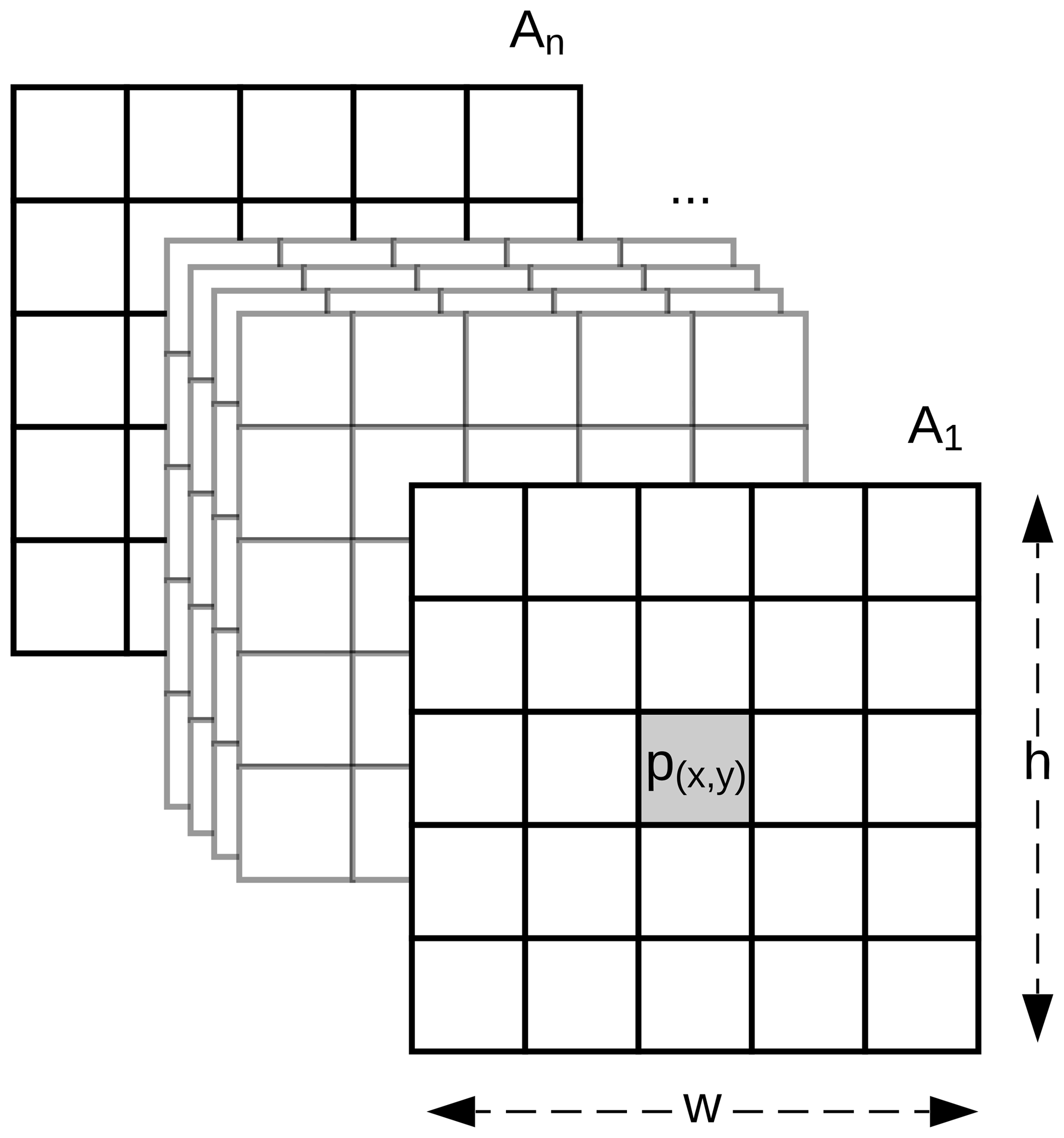
Figure 1Representation of the vicinity around a soil observation p, for n number of covariate rasters. w and h are the width and height in pixels, respectively.
Deep learning is a machine learning method that is able to learn the representation of data through a series of processing layers. In agriculture and environmental mapping, it is mainly used in hyperspectral and multispectral image classification problems, e.g. land cover classification (Kamilaris and Prenafeta-Boldú, 2018). We have not seen much application of deep learning in DSM, except for Song et al. (2016), who used the deep belief network for predicting soil moisture.
In this section we briefly introduce CNNs and some associated methods used during this work. For a more detailed and general description about CNNs we refer the reader to LeCun et al. (1990) and Krizhevsky et al. (2012).
3.1 CNN
CNNs are based on the concept of a layer of convolving windows which move along a data array in order to detect features (e.g. edges) of the data by using different filters (Fig. 2). When stacked together, convolutional layers are capable of extracting features of increasing complexity and abstraction (LeCun et al., 1990). Since CNNs have the capacity to leverage the spatial structure of the data, they have been widely and effectively used in computer vision for image recognition or extraction (LeCun and Bengio, 1995).
A CNN has a number of three-dimensional hidden layers, with each layer learning to detect different features of the input images (LeCun et al., 2015). In our case, each of the layers can perform one of the two types of operations: convolution or pooling. Convolution takes the input images through a set of convolutional filters (e.g. a 3×3 size filter), each of which detects and enhances certain features from the images. Units in a convolutional layer are organised in feature maps (here we used 3×3). Each unit of the feature map is connected to local patches in the feature maps of the previous layer through a set of weights. This local weighted sum is then passed through a non-linear transfer function.

Figure 2Example of the first three steps of a convolution of a 3×3 filter over a 5×5 array (image). The resulting pixel values correspond to the sum of the element-wise multiplication of the initial pixels (dashed lines) and the filter.
A pooling operation merges similar features by performing non-linear down-sampling. Here we used max-pooling layers which combine inputs from a small 2×2 window. Pooling also makes the features robust against noise. All the convolutional and pooling layers are finally “flattened” to the fully connected layer. In effect, the fully connected layer is a weighted sum of the previous layers.
To obtain optimal weights for the network, we train the network using a training dataset. Weights were adjusted based on a gradient-based algorithm to minimise the error using an Adam optimiser (Kingma and Ba, 2014). We refer to a review by LeCun et al. (2015) on the details of CNN.
3.2 Multi-task learning
CNNs have the capacity to predict multiple properties simultaneously. By doing so, a multi-task CNN is capable of sharing learned representations between different targets and also using the other targets as “clues” during the prediction process. In consequence, the error of the simultaneous prediction is generally lower compared with a single prediction for each target (Padarian et al., 2019; Ramsundar et al., 2015). An additional advantage of using a multi-task CNN is the reported reduction on the risk of overfitting (Ruder, 2017).
In DSM, where the combination of large extents, high resolution, and bootstrap routines leads to running multiple model realisations on billions of pixels, combined with the fact that CNNs use a group of pixels around the soil observation instead of a single pixel, the time and computational resources required for training and inference are an important factor. Due to the simultaneous training and inference of multiple targets, a multi-task CNN presents the advantage of reducing both training and inference time compared with a single-task model.
4.1 Data
The data used in this work correspond to Chilean soil information. Since most observations are distributed on agricultural lands, we complemented that information with a second small data collection compiled from the literature and collaborators. We selected soil organic carbon (SOC) content (%) at depths 0–5, 5–15, 15–30, 30–60, and 60–100 cm as our target attribute. In total, 485 soil profiles were used after excluding soil profiles with total depth lower than 100 cm (in order to assure that all the profiles have observations at all depth intervals). For more details about the data and depth standardisation we refer the reader to Padarian et al. (2017).
As covariates, we used (a) a digital elevation model (HydroSHEDS, Lehner et al., 2008), which is provided at 3 arcsec resolution, in addition to its derived slope and topographic wetness index, calculated using SAGA (Conrad et al., 2015); and (b) long-term mean annual temperature and total annual rainfall derived from information provided by WorldClim (Hijmans et al., 2005) at 30 arcsec resolution. All data layers were standardised to a 100 m grid size.
4.2 Data augmentation
Deep learning techniques are described as “data-hungry” since they usually work better with large volumes of data. The direct effect of data augmentation is to generate new samples by modifying the original data without changing its meaning (Simard et al., 2003). To achieve this, we rotated the 3-D array shown in Fig. 1 by 90, 180, and 270∘, hence quadruplicating the number of observations. It is important to note that the central pixel preserves its initial position.
A secondary effect of data augmentation is regularisation, reducing the variance of the model and overfitting (Krizhevsky et al., 2012). Data augmentation also induces rotation invariance (Vo and Hays, 2016) by generating alternative situations (rotated data) where the model response should be similar to the original data (e.g. a soil profile next to a gully is expected to be similar to a profile next to the opposite side of the gully, ceteris paribus).
4.3 Network architecture
The multi-task CNN used in this study (Fig. 3; Table 1) consists of an input layer passed through a series of convolutional and pooling layers with a ReLU (rectified linear unit) activation function, which adds non-linearity by passing the learned weights through the function . The initial common/shared network has a function of extracting features shared between the five target depth ranges. Next, the common features are propagated through independent branches, one per depth range, of three fully connected layers.
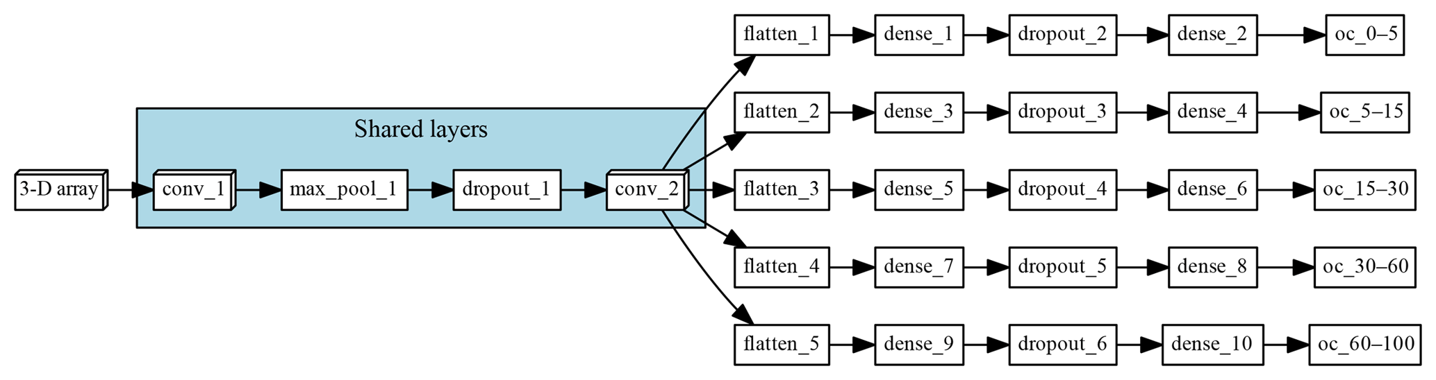
Figure 3Architecture of the multi-task network. “Shared layers” represent the layers shared by all the depth ranges. Each branch, one per depth range, first flattens the information to a 1-D array, followed by a series of two fully connected layers and a fully connected layer of size equal to 1, which corresponds to the final prediction.
The multiple connection between the layers generates a high number of parameters. In order to reduce the risk of overfitting, we introduce a dropout rate. In between the layers, 30 % of the connections were randomly disconnected (Nitish et al., 2014). We added this dropout operation in the shared layer and another dropout before the output.
Table 1Sequence of layers used to build the multi-task neural network.
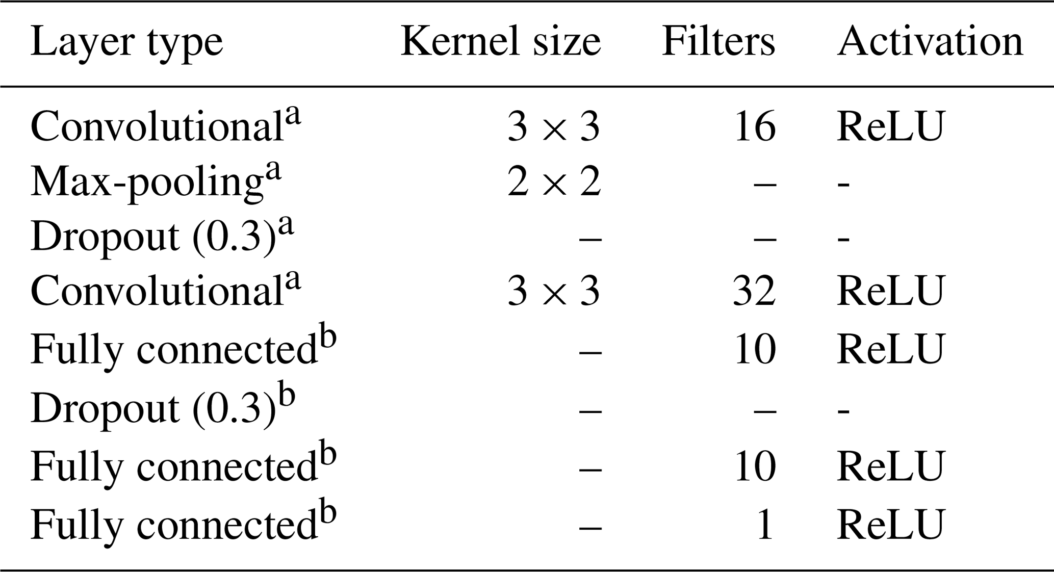
a Shared layers; b for each property.
4.4 Inputs
As explained in Sect. 2, our method uses a window around a soil observation which encloses a group of pixels instead of the single pixel that coincides with the observation. Most likely, the extent or size of that window will affect the model performance. To assess this effect, we compared the results of different models trained with a window size of 3, 5, 7, 9, 15, 21, and 29 pixels.
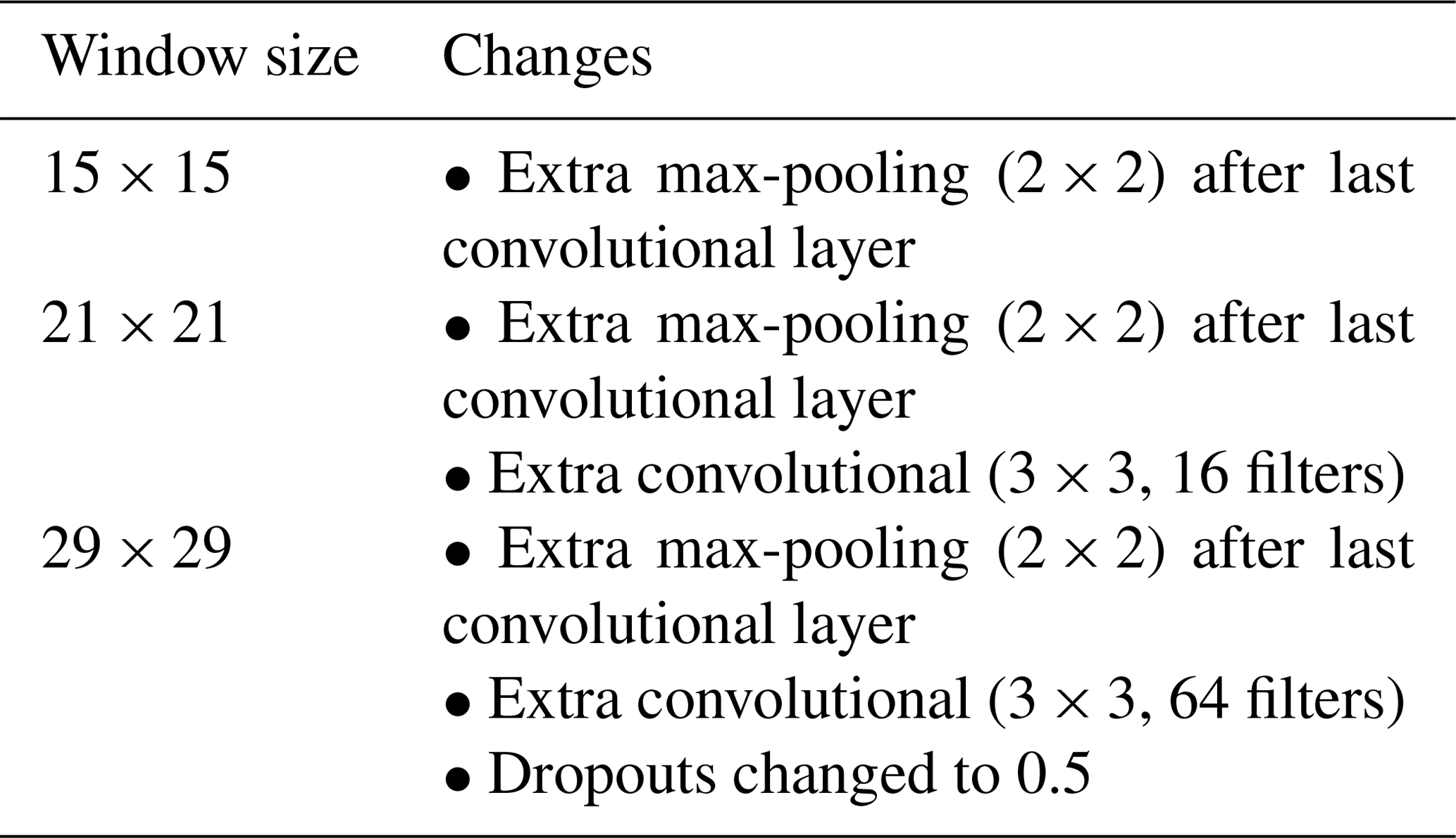
As the vicinity size increases, so does the number of parameters of the network (considering a fixed network architecture) and the risk of overfitting. To minimise overfitting, we modified the architecture of the network depending on the vicinity size (Table 2).
Table 2List of modifications made to the base network architecture for specific input window sizes.
4.5 Training and validation
First, 10 % (n=49) of the total dataset was randomly selected and used as a test set. The remaining 90 % of the samples (n=436) were augmented (see Sect. 4.2), obtaining a total of 1744 samples. Following the data augmentation, we performed a bootstrapping routine (Efron and Tibshirani, 1993) with 100 repetitions, where the training set is obtained by sampling with replacement, generating a set of size 1744. The samples which were not selected, about one-third, correspond to the out-of-bag validation set.
As a control, we compared our results with a previous study by Padarian et al. (2017) where we used a Cubist regression tree model (Quinlan, 1992) to predict soil organic carbon at a national extent. The Cubist model has been used in many other DSM studies due to its interpretability and robustness. In that study, we used the same set of soil observations and covariates described in Sect. 4.1.
4.6 Uncertainty analysis
In this work (and in Padarian et al., 2017), the uncertainty is represented as the 90 % prediction interval derived from the 100 bootstrap iterations. To estimate the upper and lower prediction interval limits, we used the following formula:
where and σ2 are the mean and variance of the 100 iterations, and MSE is the mean square error of the 100 fitted models.
4.7 Implementation
The CNN was implemented in Python (v3.6.2; Python Software Foundation, 2017) using Keras (v2.1.2; Chollet, 2015) and Tensorflow (v1.4.1; Abadi et al., 2015) back end. Computing was done using the University of Sydney's Artemis high-performance computing facility.
5.1 Data augmentation
To generalise and improve the CNN model, we created new data using only information from the training data by rotating the original image input. Data augmentation was effective at reducing model error and variability (Fig. 4). It was possible to observe a decrease in the error, by 10.56 %, 10.56 %, 11.25 %, 14.51 %, and 24.77 % for the 0–5, 5–15, 15–30, 30–60, and 60–100 cm depth ranges, respectively. The results are in accordance with image classification studies which generally showed that data augmentation increased the accuracy of classification tasks (Perez and Wang, 2017). It is hypothesised that, by increasing the amount of training data, we can reduce overfitting of CNN models.
In terms of the data spatial autocorrelation, we need to consider that after augmenting the data we have four samples in the same locations with exactly the same SOC content, therefore assuming that there is no variance when distance is equal to 0. That is theoretically true if we consider that the distance is exactly equal to 0. In practice, when calculating the semivariogram, the semivariance value of the first bin will be lower, but that does not significantly affect the final model.

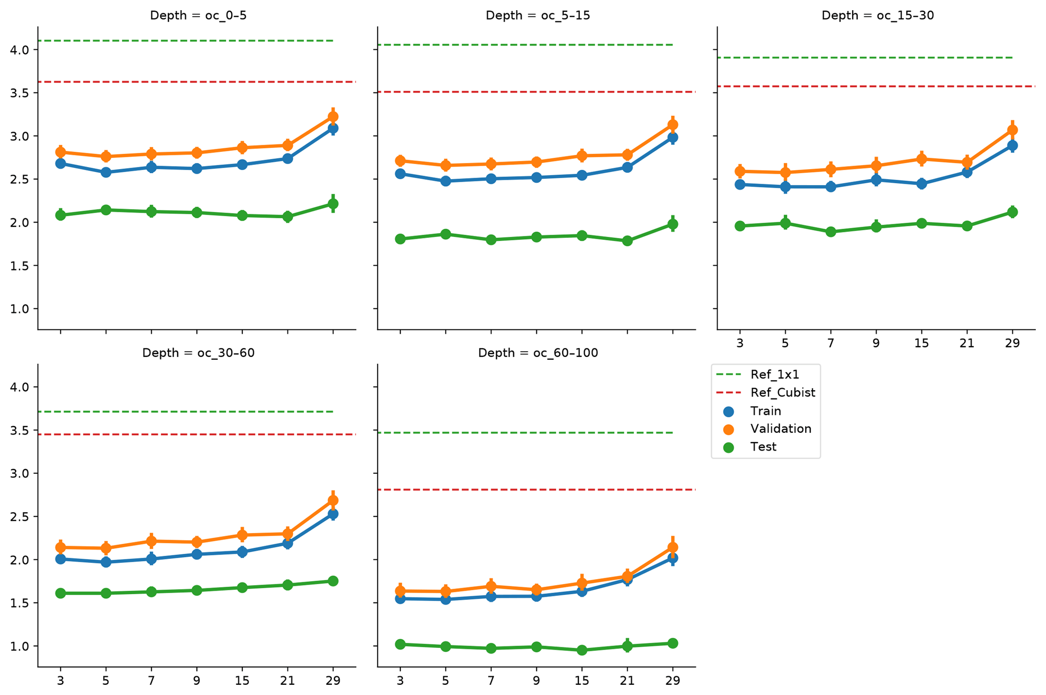
Figure 5Effect of vicinity size on prediction error, by depth range. Ref_1×1 corresponds to a fully connected neural network without any surrounding pixels. Ref_Cubist corresponds to the Cubist models used by Padarian et al. (2017).
5.2 Vicinity size
To incorporate contextual information for DSM prediction, we represent the input as an image. The image is represented as observation in the centre, with surrounding pixels in a square format. The size of the neighbourhood window (vicinity) has a significant effect on the prediction error (Fig. 5). There is no significant difference when using a vicinity size of 3, 5, 7, or 9 pixels, but sizes above 9 pixels showed an increase in the error. It is possible to observe a lower error in the test dataset, compared with the training and validation, due to the slight differences in the dataset distributions (Fig. 6). Since the SOC distribution is right-skewed, the random sampling used to generate the training dataset does not completely recreate the original distribution, excluding samples with very high SOC values. This should not significantly affect the conclusions given that the error for the samples with hight SOC values is accounted for during the bootstrapping routine and reflected in the training and validation curves of Fig. 5. In this example, for a country-scale mapping of SOC at 100 m grid size, information from a 150 to 450 m radius is useful. A similar influence distance was obtained by Jian-Bing et al. (2006) and Sun et al. (2003), who reported a medium-scale spatial correlation range for SOC in China of around 300 and 550 m, respectively; by Rossi et al. (2009), who reported a range of around 190 m for a coastal forest in Tanzania; and by Don et al. (2007), who reported a range of around 200 m in two grassland sites in Germany. A similar spatial correlation range was reported for croplands in an review by Paterson et al. (2018), where, based on 41 variograms, the authors estimated an average spatial correlation range of around 400 m.

Figure 6Distribution of the original dataset and the test dataset. The random sampling excludes some observation with high SOC values.
As described in Sect. 4.3, we slightly modified the architecture of the network as input window size increased, in order to minimise the risk of overfitting and isolate the effect of the vicinity size. As we increase the vicinity size, we give the model a broader spatial context. Our results show that just a small amount of extra context provides enough information to improve the model predictions, and a larger amount of neighbouring information acts as noise, impairing the generalisation of the model. Since we used the relatively large resolution of 100 m, it is hard to tell specifically what the minimum amount of context needed to improve SOC predictions is. We believe that using higher resolutions (<10 m) could produce more insights about this matter.
Soil-forming factors interact in complex ways and affect soil properties with different strength. At the local scale, a broader context (i.e. larger vicinity size) does not necessarily provide extra information to the model, for instance when one of the factors is relatively homogeneous. The extra information could be even detrimental if the vicinity size is well beyond the area of influence of a factor, which is what probably happened when we increased the vicinity size above 9 pixels (radius ≈450 m). Representing this complexity in numerical terms would imply varying the size of the input array, such as a different vicinity size for each forming factor, most likely also varying depending on the spatial location of the soil observation (e.g. smaller vicinity for homogeneous areas and larger for heterogeneous areas). This is technically possible but considerably increases the complexity of the modelling.
5.3 Comparison with other methods
We compared our approach with the Cubist model used in our previous study (Padarian et al., 2017), where we did not use any contextual information. We observed a significant decrease in the error (Fig. 5) by 23.0 %, 23.8 %, 26.9 %, 35.8 %, and 39.8 % for the 0–5, 5–15, 15–30, 30–60, and 60–100 cm depth ranges, respectively. Most current DSM studies rely on punctual observations without contextual information, and, given the improvements shown by our approach, we believe there is a big potential for CNNs to be used in operational DSM.
To compare our results with a method that uses contextual information, we ran a test using wavelet decomposition as per Mendonça-Santos et al. (2006). In addition to the five covariates, we used their approximation coefficients from the first, second, and third levels of a Haar decomposition (Chui, 2016; Haar, 1910). The results including wavelet-decomposed variables were similar to ones obtained with the Cubist model. The CNN approach reduced the error by 24.8, 24.7, 28.5, 28.6, and 23.5 for the 0–5, 5–15, 15–30, 30–60, and 60–100 cm depth ranges, respectively. Mendonça-Santos et al. (2006) reported an average improvement of 1 % for the prediction of clay content. In our case the wavelet decomposition reduced the error of the SOC content by 5.1 %, on average, compared with the Cubist model, but the reduction was only observed in depth, where SOC content is low (2.4 %, 1.2 %, 2.3 %, −10.1 %, and −21.4 % error change for the 0–5, 5–15, 15–30, 30–60, and 60–100 cm depth ranges, respectively), hence reducing the effect in applications such as carbon accounting. Our approach showed greater error reductions and through the whole profile.
5.4 Prediction of deeper soil layers
Our approach uses a multi-task CNN to predict multiple depths simultaneously in order to produce a synergistic effect. Compared with predicting each depth range in isolation by training a network with the same structure (Sect. 4.3) but with only one output, our approach reduced the error by 1.5 %, 6.7 %, 6.6 %, 8.9 %, and 13.0 % for the 0–5, 5–15, 15–30, 30–60, and 60–100 cm depth ranges, respectively. In this case, the reduction was modest and we believe the effect can be greater when more soil observations are available.
In DSM, there are two main approaches to deal with the vertical variation of a soil attribute: 2.5-D and 3-D modelling. In the first one, an independent model is fitted for each depth range. The latter explicitly incorporates depth in order to obtain a single model for the whole profile. Interestingly, both approaches show a decrease in the variance explained by the model as the prediction depth increases. In a 3-D mapping of SOC for a 125 km2 region in the Netherlands, Kempen et al. (2011) presented R2 values of 0.75, 0.23, and 0.09 for the 0–30, 30–60, and 60–90 cm depth ranges, respectively. In our previous study (Padarian et al., 2017), the 2.5-D mapping showed R2 values of 0.39, 0.39, 0.27, 0.19, and 0.17 for the 0–5, 5–15, 15–30, 30–60, and 60–100 cm depth ranges, respectively. Similar studies show the same trend (Akpa et al., 2016; Mulder et al., 2016; Adhikari et al., 2014), independent of the models used or the soil attribute predicted. This is expected as the information used as covariates usually represents surface conditions. Our multi-task network presented the opposite trend (Fig. 7), showing an increase in the explained variance as the prediction depth increases.
The prediction of the adjacent layers served as guidance, producing a synergistic effect. A soil attribute through a profile usually has a predictable behaviour (unless there are lithological discontinuities), which has been described by many authors in the form of depth functions (Kempen et al., 2011; Nakane, 1976; Russell and Moore, 1968). A CNN is capable of generating an internal representation of the vertical distribution of the target attribute, which resembles the observed pattern (Fig. 8).
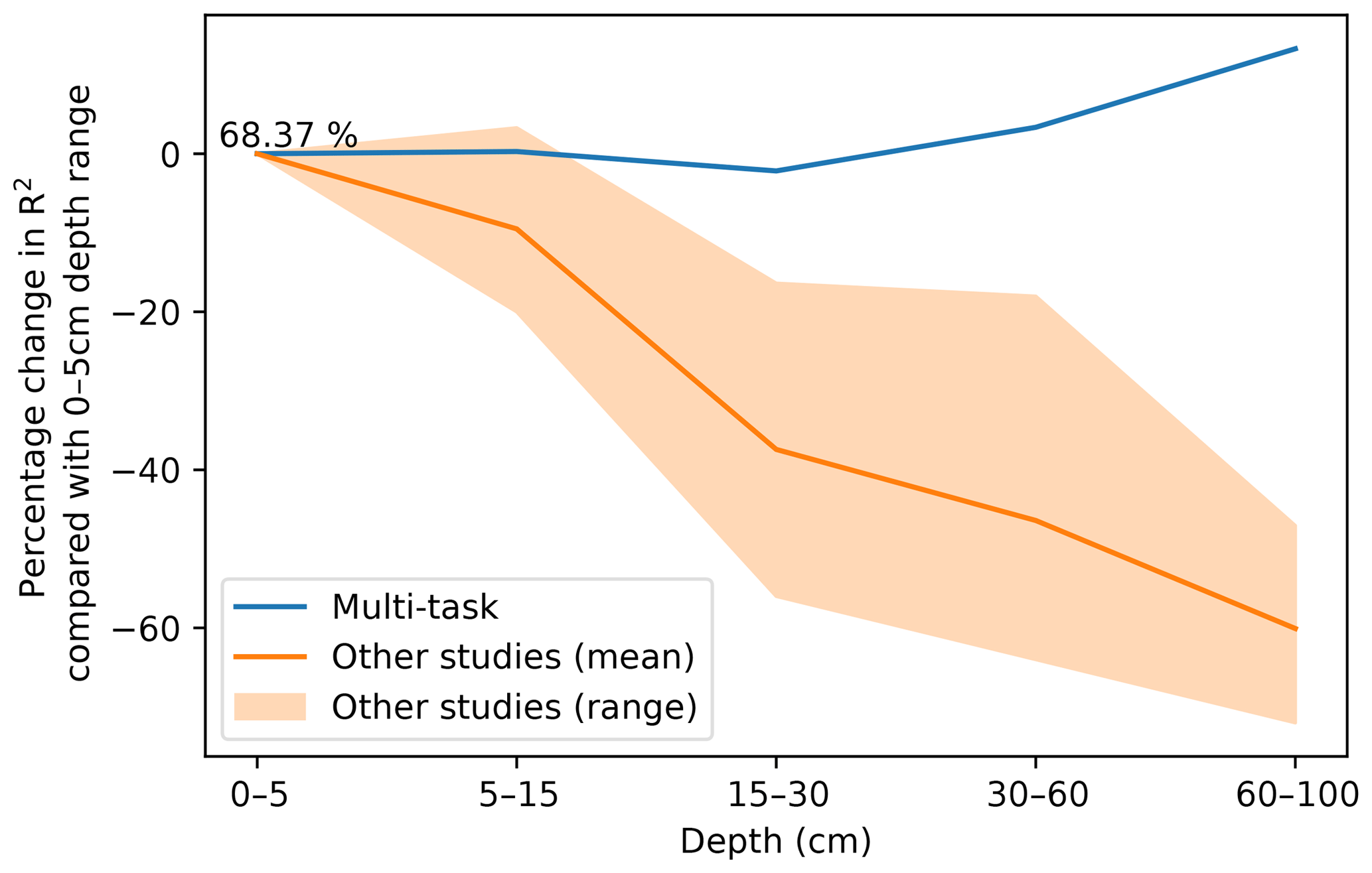
Figure 7Percentage change in model R2 as a function of depth. The multi-task model corresponds to a CNN trained using a 7 pixel × 7 pixel vicinity. Data for “other studies” correspond to validation statistics from Padarian et al. (2017), Akpa et al. (2016), Mulder et al. (2016), and Adhikari et al. (2014).
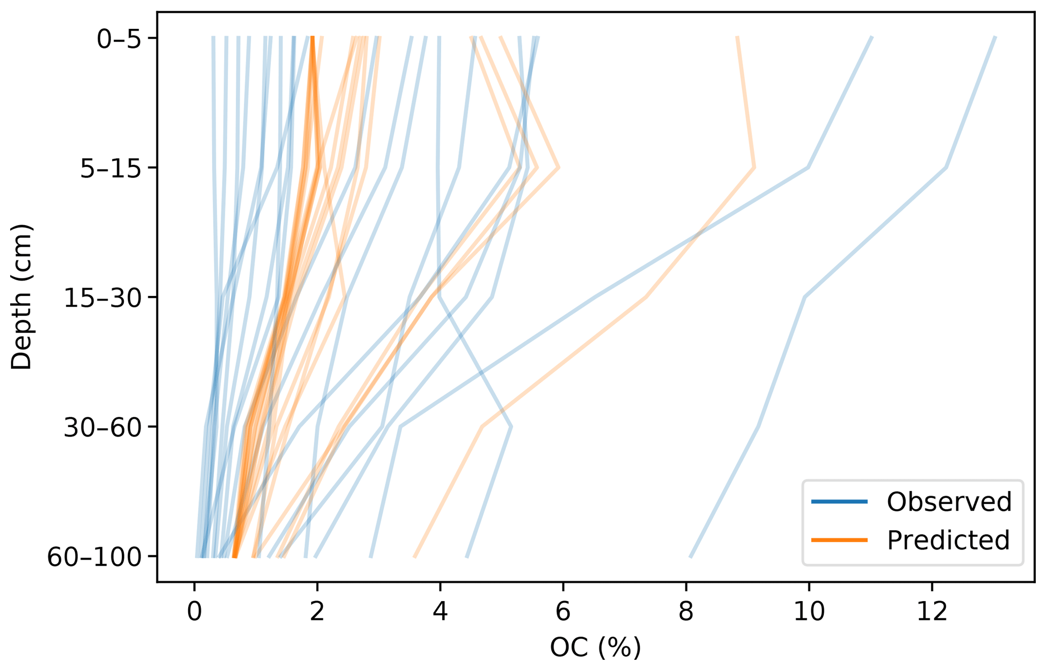
Figure 8Vertical SOC distribution for 20 randomly selected profiles. Predictions correspond to the multi-task CNN.
5.5 Visual evaluation of maps
Visually, the maps generated with the Cubist tree model and our multi-task CNN showed differences (Fig. 9). In an example for an area in southern Chile (around 72.57∘ S), the map generated with the Cubist model (Fig. 9a) shows more details related with the topography, but also presents some artefacts due to the sharp limits generated by the tree rules. On the other hand, the map generated with the multi-task CNN using a 7×7 window (Fig. 9b) shows a smoothing effect, which is an expected behaviour consequence of using neighbour pixels.
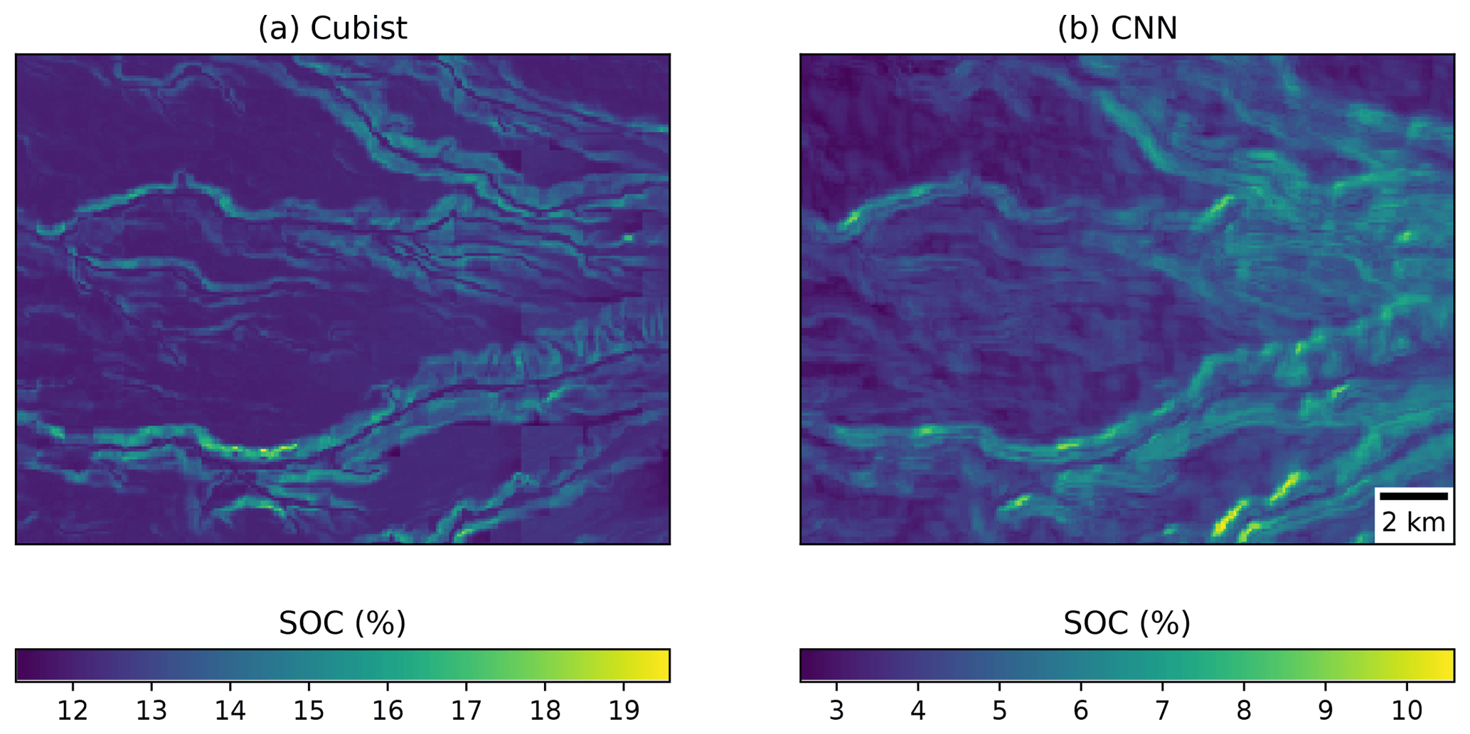
Figure 9Detailed view of the (a) map generated by a Cubist model (Padarian et al., 2017) and (b) model generated by our multi-task CNN showing the smoothing effect of the CNN.
5.6 Uncertainty
A recommended DSM practice is to present a map of a predicted attribute along its associated uncertainty (Arrouays et al., 2014). Our multi-task CNN significantly reduced the prediction interval width (PIW, Table 3) compared with the Cubist model. On average, we observed a reduction of 13.8 % and 13.1 % for the CNN model generated with and without data augmentation pretreatment, respectively, for the first three depth intervals. Our multi-task CNN model showed a slightly lower prediction interval coverage, but all were wider than the proposed 90 % coverage.
In terms of the spatial patterns of the uncertainty (Fig. 10), the greater reductions of the PIW were observed in elevated areas of the Andes, followed by the central valleys. A slight increase, on the order of 6 %–8 %, was observed in the western coastal ranges. The reduction of the PIW in the Andes is most likely due to a more reserved extrapolation by the CNN models compared with the Cubist model. It is worth noting that the central valleys are where most of the agricultural lands are located and the uncertainty reduction observed in these areas could have important implications.
Table 3Median prediction interval width (PIW, SOC %) and proportion of observations that fell within the 90 % prediction interval (PICP) estimated at the test dataset locations. For the Cubist model, values were extracted from the final maps. For the CNN models, the values correspond to the mean of the 100 bootstrap iterations.
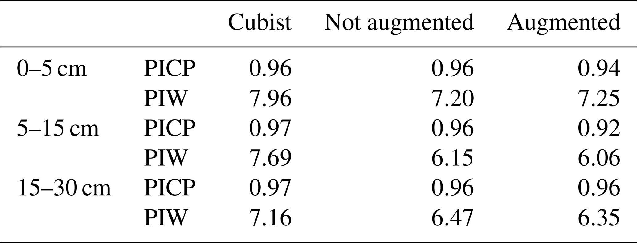
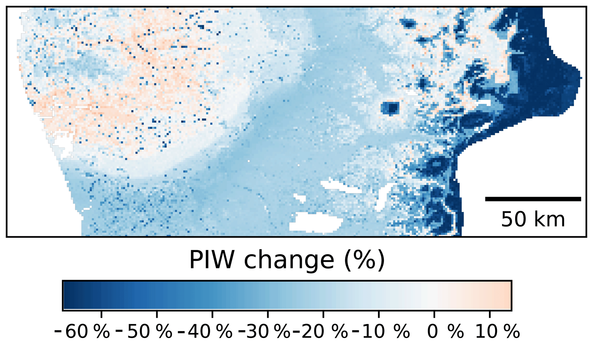
Figure 10Percentage change on the prediction interval width using as a reference a Cubist model (Padarian et al., 2017). Comparison made using data augmentation pretreatment.
The incorporation of contextual information into DSM models is an important aspect that deserves more attention. Since a soil surveyor will look at the surrounding landscape to make a prediction of soil type, DSM models should also incorporate information surrounding an observation. We demonstrated the use of a convolutional neural network as an efficient, effective, and accurate method to achieve this goal. In particular we introduce a deep learning model for DSM which has the following innovative features:
-
The representation of input as an image, which takes into account information surrounding a point observation. CNN is able to recognise contextual information and extract multi-scale information automatically, which circumvents the need to preprocess the data in the form of spatial filtering or multi-scale analysis.
-
The use of data augmentation as a general representation of soil in the landscape, which can reduce overfitting and improve model accuracy.
-
The ability to predict different soil depth simultaneously in a model and thus take into account the depth correlation of soil properties and attributes. In our example, the prediction of soil properties at deeper layers, which is a common problem in DSM studies, improved significantly.
Overall, in this study, we observed an error reduction of 30 % compared with conventional techniques. The resulting prediction also has less uncertainty. Furthermore, the use of this data structure with CNN seems to eliminate artefacts generally found in DSM products due to the incompatible scale of covariates and sharp discontinuities due to tree models.
A CNN can handle a large number of covariates and has advantages over other machine learning algorithms used in DSM, such as random forests and Cubist regression tree models, because its architecture is flexible and explicitly takes spatial information of covariates around observations. While there have been attempts to include information surrounding an observation as covariates in a random forest model, those inputs still do not have a spatial relationship. CNN does not require preprocessing such as wavelet transformation, rather such a function is built into the model. There are other features such as handling missing values via data imputation (Duan et al., 2016) which can be readily added in the network.
The example presented in this paper is for a country-wide modelling at 100 m resolution, and we need to further test such an approach in the regional to landscape mapping. The CNN model would be highly suitable for mapping soil class. In addition, the presented model can be used for other environmental mapping.
The data were manually extracted from books, which are publicly available and cited on Padarian (2017).
The authors declare that they have no conflict of interest.
This research was supported by Sydney Informatics Hub, funded by the University of Sydney.
Edited by: Bas van Wesemael
Reviewed by: two anonymous referees
Abadi, M., Agarwal, A., Barham, P., Brevdo, E., Chen, Z., Citro, C., Corrado, G. S., Davis, A., Dean, J., Devin, M., Ghemawat, S., Goodfellow, I., Harp, A., Irving, G., Isard, M., Jia, Y., Jozefowicz, R., Kaiser, L., Kudlur, M., Levenberg, J., Mané, D., Monga, R., Moore, S., Murray, D., Olah, C., Schuster, M., Shlens, J., Steiner, B., Sutskever, I., Talwar, K., Tucker, P., Vanhoucke, V., Vasudevan, V., Viégas, F., Vinyals, O., Warden, P., Wattenberg, M., Wicke, M., Yu, Y., and Zheng, X.: TensorFlow: Large-Scale Machine Learning on Heterogeneous Systems, available at: https://www.tensorflow.org/ (last access: 22 February 2019), 2015. a
Adhikari, K., Hartemink, A. E., Minasny, B., Kheir, R. B., Greve, M. B., and Greve, M. H.: Digital mapping of soil organic carbon contents and stocks in Denmark, PloS one, 9, e105519, https://doi.org/10.1371/journal.pone.0105519, 2014. a, b
Akpa, S. I., Odeh, I. O., Bishop, T. F., Hartemink, A. E., and Amapu, I. Y.: Total soil organic carbon and carbon sequestration potential in Nigeria, Geoderma, 271, 202–215, 2016. a, b
Angelini, M. E. and Heuvelink, G. B.: Including spatial correlation in structural equation modelling of soil properties, Spat. Stat.-Nath., 25, 35–51, 2018. a
Angelini, M., Heuvelink, G., and Kempen, B.: Multivariate mapping of soil with structural equation modelling, Eur. J. Soil Sci., 68, 575–591, 2017. a
Arrouays, D., McBratney, A., Minasny, B., Hempel, J., Heuvelink, G., MacMillan, R., Hartemink, A., Lagacherie, P., and McKenzie, N.: The GlobalSoilMap project specifications, in: GlobalSoilMap: Basis of the Global Spatial Soil Information System – Proceedings of the 1st GlobalSoilMap Conference, edited by: Arrouays D., McKenzie, N., Hempel, J., Richer de Forges, A., and McBratney, A. B., Orleans, France, 7–9 October 2013, CRC Press, 9–12, https://doi.org/10.1201/b16500-4, 2014. a, b
Behrens, T., Schmidt, K., Zhu, A.-X., and Scholten, T.: The ConMap approach for terrain-based digital soil mapping, Eur. J. Soil Sci., 61, 133–143, 2010. a, b, c
Behrens, T., Schmidt, K., Ramirez-Lopez, L., Gallant, J., Zhu, A.-X., and Scholten, T.: Hyper-scale digital soil mapping and soil formation analysis, Geoderma, 213, 578–588, 2014. a, b
Behrens, T., Schmidt, K., MacMillan, R., and Rossel, R. V.: Multiscale contextual spatial modelling with the Gaussian scale space, Geoderma, 310, 128–137, 2018. a
Biswas, A. and Si, B. C.: Revealing the controls of soil water storage at different scales in a hummocky landscape, Soil Sci. Soc. Am. J., 75, 1295–1306, 2011. a
Chen, S., Martin, M. P., Saby, N. P., Walter, C., Angers, D. A., and Arrouays, D.: Fine resolution map of top-and subsoil carbon sequestration potential in France, Sci. Total Environ., 630, 389–400, 2018. a
Chollet, F.: Keras, available at: https://github.com/fchollet/keras (last access: 22 February 2019), 2015. a
Chui, C. K.: An introduction to wavelets, Elsevier, Noston, MA, USA, 2016. a
Conrad, O., Bechtel, B., Bock, M., Dietrich, H., Fischer, E., Gerlitz, L., Wehberg, J., Wichmann, V., and Böhner, J.: System for Automated Geoscientific Analyses (SAGA) v. 2.1.4, Geosci. Model Dev., 8, 1991–2007, https://doi.org/10.5194/gmd-8-1991-2015, 2015. a
Demattê, J. A. M., Fongaro, C. T., Rizzo, R., and Safanelli, J. L.: Geospatial Soil Sensing System (GEOS3): A powerful data mining procedure to retrieve soil spectral reflectance from satellite images, Remote Sens. Environ., 212, 161–175, 2018. a
Deumlich, D., Schmidt, R., and Sommer, M.: A multiscale soil–landform relationship in the glacial-drift area based on digital terrain analysis and soil attributes, J. Plant Nutr. Soil Sc., 173, 843–851, 2010. a
Dokuchaev, V. V.: Russian Chernozem. Selected works of V. V. Dokuchaev. v. 1, Israel Program for Scientific Translations, Jerusalem, Israel, 1883 (translated in 1967). a
Don, A., Schumacher, J., Scherer-Lorenzen, M., Scholten, T., and Schulze, E.-D.: Spatial and vertical variation of soil carbon at two grassland sites – implications for measuring soil carbon stocks, Geoderma, 141, 272–282, 2007. a
Duan, Y., Lv, Y., Liu, Y.-L., and Wang, F.-Y.: An efficient realization of deep learning for traffic data imputation, Transport. Res. C-Emer, 72, 168–181, 2016. a
Efron, B. and Tibshirani, R. J.: An introduction to the bootstrap, vol. 57, CRC press, New York, USA, 1993. a
Haar, A.: Zur theorie der orthogonalen funktionensysteme, Math. Ann., 69, 331–371, 1910. a
Hijmans, R. J., Cameron, S. E., Parra, J. L., Jones, P. G., and Jarvis, A.: Very high resolution interpolated climate surfaces for global land areas, Int. J. Climatol., 25, 1965–1978, 2005. a
Jenny, H.: Factors of soil formation: a system of quantitative pedology,, Macgraw Hill, New York 1941. a
Jian-Bing, W., Du-Ning, X., Xing-Yi, Z., Xiu-Zhen, L., and Xiao-Yu, L.: Spatial variability of soil organic carbon in relation to environmental factors of a typical small watershed in the black soil region, northeast China, Environ. Monit. Assess., 121, 597–613, 2006. a
Kamilaris, A. and Prenafeta-Boldú, F. X.: Deep learning in agriculture: A survey, Comput. Electron. Agr., 147, 70–90, 2018. a
Kempen, B., Brus, D., and Stoorvogel, J.: Three-dimensional mapping of soil organic matter content using soil type–specific depth functions, Geoderma, 162, 107–123, 2011. a, b
Keskin, H. and Grunwald, S.: Regression kriging as a workhorse in the digital soil mapper's toolbox, Geoderma, 326, 22–41, 2018. a
Kingma, D. and Ba, J.: Adam: A method for stochastic optimization, arXiv preprint arXiv:1412.6980, 2014. a
Krizhevsky, A., Sutskever, I., and Hinton, G. E.: Imagenet classification with deep convolutional neural networks, in: Advances in neural information processing systems, MIT Press, 1097–1105, 2012. a, b
LeCun, Y., Boser, B. E., Denker, J. S., Henderson, D., Howard, R. E., Hubbard, W. E., and Jackel, L. D.: Handwritten digit recognition with a back-propagation network, in: Advances in neural information processing systems, MIT Press, 396–404, 1990. a, b
LeCun, Y. and Bengio, Y., : Convolutional networks for images, speech, and time series, The handbook of brain theory and neural networks, MIT Press, 3361, 1995. a
LeCun, Y., Bengio, Y., and Hinton, G.: Deep learning, Nature, 521, 436–444, 2015. a, b
Lee, H. and Kwon, H.: Going deeper with contextual CNN for hyperspectral image classification, IEEE T. Image Process., 26, 4843–4855, 2017. a
Lehner, B., Verdin, K., and Jarvis, A.: New global hydrography derived from spaceborne elevation data, EOS, Transactions American Geophysical Union, 89, 93–94, 2008. a
McBratney, A., Mendonça Santos, M. L., and Minasny, B.: On digital soil mapping, Geoderma, 117, 3–52, 2003. a
Mendonça-Santos, M., McBratney, A., and Minasny, B.: Soil prediction with spatially decomposed environmental factors, Dev. Soil Sci., 31, 269–278, 2006. a, b, c
Miller, B. A., Koszinski, S., Wehrhan, M., and Sommer, M.: Impact of multi-scale predictor selection for modeling soil properties, Geoderma, 239, 97–106, 2015. a
Mulder, V., Lacoste, M., de Forges, A. R., and Arrouays, D.: GlobalSoilMap France: High-resolution spatial modelling the soils of France up to two meter depth, Sci. Total Environ., 573, 1352–1369, 2016. a, b
Nakane, K.: An empirical formulation of the vertical distribution of carbon concentration in forest soils, Japanese Journal of Ecology, 26, 171–174, 1976. a
Nitish, S., Hinton, G. E., Krizhevsky, A., Sutskever, I., and Salakhutdinov, R.: Dropout: a simple way to prevent neural networks from overfitting., J. Mach. Learn. Res., 15, 1929–1958, 2014. a
Padarian, J., Minasny, B., and McBratney, A.: Chile and the Chilean soil grid: a contribution to GlobalSoilMap, Geoderma Regional, 9, 17–28, 2017. a, b, c, d, e, f, g, h, i
Padarian, J., Minasny, B., and McBratney, A.: Using deep learning to predict soil properties from regional spectral data, Geoderma Regional, 16, e00198, https://doi.org/10.1016/j.geodrs.2018.e00198, 2019. a
Paterson, S., McBratney, A. B., Minasny, B., and Pringle, M. J.: Variograms of Soil Properties for Agricultural and Environmental Applications, in: Pedometrics, Springer, Cham, Switzerland, 623–667, 2018. a
Perez, L. and Wang, J.: The effectiveness of data augmentation in image classification using deep learning, arXiv preprint arXiv:1712.04621, 2017. a
Poggio, L. and Gimona, A.: Assimilation of optical and radar remote sensing data in 3D mapping of soil properties over large areas, Sci. Total Environ., 579, 1094–1110, 2017. a
Python Software Foundation: Python Language Reference, Python Software Foundation, available at: https://www.python.org (last access: 22 February 2019), 2017. a
Quinlan, J. R.: Learning with continuous classes, in: 5th Australian joint conference on artificial intelligence, Singapore, 16–18 November 1992, vol. 92, 343–348, 1992. a
Ramsundar, B., Kearnes, S., Riley, P., Webster, D., Konerding, D., and Pande, V.: Massively multitask networks for drug discovery, arXiv preprint arXiv:1502.02072, 2015. a
Rossi, J., Govaerts, A., De Vos, B., Verbist, B., Vervoort, A., Poesen, J., Muys, B., and Deckers, J.: Spatial structures of soil organic carbon in tropical forests—a case study of Southeastern Tanzania, Catena, 77, 19–27, 2009. a
Ruder, S.: An overview of multi-task learning in deep neural networks, arXiv preprint arXiv:1706.05098, 2017. a
Russell, J. S. and Moore, A. W.: Comparison of different depth weighting in the numerical analysis of anisotropic soil profile data, in: Transactions of the 9th International Congress Soil Science, Adelaide, Sydney, International Soil Science Society, 205–213, 1968. a
Simard, P. Y., Steinkraus, D., and Platt, J. C.: Best practices for convolutional neural networks applied to visual document analysis, Seventh International Conference on Document Analysis and Recognition, Edinburgh, UK, 2003, vol. 3, 958–962, 2003. a
Somarathna, P., Minasny, B., and Malone, B. P.: More Data or a Better Model? Figuring Out What Matters Most for the Spatial Prediction of Soil Carbon, Soil Sci. Soc. Am. J., 81, 1413–1426, https://doi.org/10.2136/sssaj2016.11.0376, 2017. a
Song, X., Zhang, G., Liu, F., Li, D., Zhao, Y., and Yang, J.: Modeling spatio-temporal distribution of soil moisture by deep learning-based cellular automata model, J. Arid Land, 8, 734–748, 2016. a, b
Sun, B., Zhou, S., and Zhao, Q.: Evaluation of spatial and temporal changes of soil quality based on geostatistical analysis in the hill region of subtropical China, Geoderma, 115, 85–99, 2003. a
Sun, X.-L., Wang, H.-L., Zhao, Y.-G., Zhang, C., and Zhang, G.-L.: Digital soil mapping based on wavelet decomposed components of environmental covariates, Geoderma, 303, 118–132, 2017. a, b
Vo, N. N. and Hays, J.: Localizing and orienting street views using overhead imagery, in: European Conference on Computer Vision, Amsterdam, the Netherlands, Springer, 494–509, 2016. a