Soil indicators for ecosystem services: a focus on water regulation

Soil health assessments increasingly rely on indicators to infer soil functions and ecosystem services; however, the extent to which these indicators accurately represent water-related soil processes remains uncertain. This study investigates the relationships between soil properties and provision of water regulation ecosystem services across three contrasting pedo-climatic regions in Austria, Italy, and Tunisia. Using 315 soil profiles, we applied a process-based soil–water model to quantify infiltration, runoff triggering, groundwater recharge, and crop water stress index under representative climatic conditions. We evaluated commonly used soil indicators, including saturated hydraulic conductivity, available water content, bulk density, organic matter content, clay content, saturated soil water content, soil depth, and macroporosity. Pairwise correlation and multiple linear regression analyses were employed to assess interactions between soil properties and soil water balance components. Results show that indicator–process relationships vary considerably across sites and are often non-linear, with specific correlations reflecting local combinations of soil texture, structure, profile development, and climate. For example, in the Marchfeld region (Austria), infiltration exhibited a strong positive correlation with bulk density (r=0.74, p<0.001), while the crop water stress index showed a significant negative correlation with soil depth (r= −0.35, p<0.001). In the Bologna area (Italy), the study also indicated that groundwater recharge was positively correlated with soil macro-porosity (r=0.45, p<0.001), whereas macro-porosity exhibited a strong negative correlation with flux-to-runoff (r= −0.66, p<0.001), underscoring the key role of soil structural characteristics in controlling infiltration–recharge–runoff dynamics. In addition, multiple linear regression models were developed to assess the relevance of the individual soil properties and their interactions in controlling soil water balance components. For instance, the infiltration model for Marchfeld (r=0.79, p<0.001) was highly predictive and incorporated clay content, organic matter, and soil depth. Several widely used indicators exhibited weaker or inconsistent relationships with water-related processes than commonly assumed. For instance, saturated hydraulic conductivity alone was not a robust predictor of infiltration and recharge across sites, whereas soil depth and clay content emerged as recurrent controls, especially when considered jointly. Overall, this study highlights the value of process-based modelling for disentangling soil–climate interactions and cautions against the generalized use of static soil indicators in hydrological and soil health assessments.

1 Introduction

Soil delivers a wide range of high-value functions, including food production, raw material supply, support for human activities, historical archiving, biodiversity conservation, organic carbon sequestration, and regulation of water and nutrient cycles (McBratney et al., 2017).

In fulfilling these functions, soils provide a variety of goods and services essential to human well-being and the advancement of sustainable socio-economic development, collectively known as “ecosystem services” (Costanza et al., 1997).

Despite soil’s importance as a key component of terrestrial ecosystems, most studies – especially in the past – have focused on ecosystem services, such as provisioning, supporting, regulating, and cultural services, stemming from other ecosystem components, while placing little emphasis on soil itself (Costanza et al., 1997; MEA, 2005; Hewitt et al., 2015).

A decade ago, this represented the state of the art; however, significant progress has been made since then. Numerous projects and initiatives have emerged to highlight and deepen our understanding of the mechanisms driving the delivery of soil-based ecosystem services. Notable examples include the SERENA project (https://ejpsoil.eu/soil-research/serena, last access: 12 January 2025), the SOB4ES project (https://www.sob4es.eu/, last access: 12 January 2025), the SOILS4MED project (https://mel.cgiar.org/projects/1866, last access: 13 January 2025), and the BENCHMARKS project (https://soilhealthbenchmarks.eu/, last access: 22 December 2024) at the EU level, as well as the Global Soil Biodiversity Initiatives network (https://www.globalsoilbiodiversity.org/, last access: 20 December 2024) at the global level.

More recently, emphasis has been placed on linking ecosystem services and soil functions with the state of soil health. For example, in Europe the EU soil strategy for 2030 (SWD, 2021) stated that “soils are healthy when they are in good chemical, biological, and physical condition and are able to continuously provide as many of the ecosystem services as possible”. As schematically illustrated in Fig. 1, the assessment of soil health follows, in principle, several sequential steps that require increasing levels of integration. This assessment begins with the measurement of basic soil parameters, which are used to evaluate the physical, chemical, and biological processes they regulate. These processes are then progressively translated into estimates of soil ecosystem services, and their combined evaluation ultimately leads to an integrated assessment of overall soil health. In practice, to achieve the goal of effectively evaluating soil health, there has been a notable increase in efforts to identify straightforward indicators and indices that can serve as proxies for soil processes, soil functions, and ecosystem services, thereby reflecting the overall health of soil in a simplified manner. Among the many studies on this topic, a few key bibliographic and review works include those by Bünemann et al. (2018), Rinot et al. (2019), Jian et al. (2020), Liu et al. (2020), Bagnall et al. (2023), Sellami and Terribile (2023), and Sellami et al. (2025).

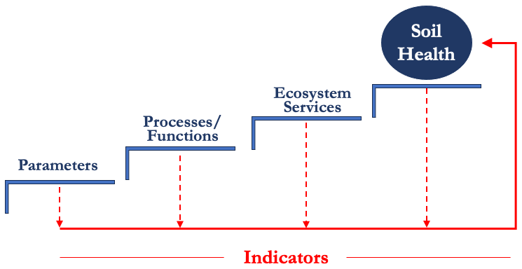
Figure 1 Schematic linkage of soil parameters, processes, functions, ecosystem services and indicators for soil health assessment

The inherent complexity of soil and the interconnected functions resulting in the processes underpinning the delivery of soil-based ecosystem services hamper to some extent the efficacy of few indicators, which by definition are static and are based on a more or less limited set of soil properties, which are assumed to be directly linked to a soil process, function, and ecosystem service. On one hand, holistic approaches to soil indicators (e.g., Dominati et al., 2016; Costantini et al., 2016) have successfully allowed the definition of theoretical frameworks for the integration of soil-based ecosystem services into policy and land planning (e.g., the EU Soil Monitoring Law, officially entering force 16 December 2025), on the other hand, there is the risk of overlooking the actual complexity of field dynamics and their temporal variability. A step forward in addressing soil’s multi-functionality and variability requires quantifying multiple indicators and integrating them into a comprehensive index. However, as Lehmann et al. (2020) highlighted in their review of over 500 studies on soil health and quality, relatively few indices exist, with only five studies including a single soil health index. The limitation of inferring soil health solely from indicators (Fig. 1) lies in overlooking the dynamic nature of soil, a complex time-dependent system (Lal, 2008). This is especially true for water-regulating services, where the dynamic component plays a critical role. In fact, the quantification and comprehensive study of water regulation services remain under exploration, highlighting the need for further research on the role of soils in hydrological regulation. Here we provide examples of studies examining soil health in relation to water regulation services. Moebius-Clune et al. (2016) used wet aggregate stability and Available Water Content (AWC) as key indicators. Bagnall et al. (2022b) found that doubling soil organic carbon could nearly double the water storage capacity of soil. Another study by Bagnall et al. (2022a) tested several parameters – such as water-stable aggregate percentage, bulk density, permanent wilting point, field capacity (measured on both repacked and intact cores), saturated hydraulic conductivity, and soil organic carbon, revealing that field capacity measured on intact soil cores was the best indicator of soil physical health in relation to the water cycle. As part of the EU SERENA project under EJP Soil (https://ejpsoil.eu/soil-research/serena, last access: 12 January 2025), information was collected on existing methods across 14 member states for evaluating soil-based ecosystem services. For water regulation services (termed “hydrological control”), assessments primarily focused on AWC, followed by water groundwater recharge, evapotranspiration, runoff, and saturated hydraulic conductivity.

As previously highlighted, a substantial body of research investigates the relationships among indicators, processes, ecosystem services, and soil health. However, the extent to which an indicator represents a specific process is often assumed to be uniform across soils or derived from simplified schemes. Such schemes frequently overlook the vertical variability of soil properties – particularly hydrological characteristics – by presuming soil homogeneity. Furthermore, the climatic component plays a crucial role in driving the dynamic nature of soil processes, thereby influencing the parameters and indicators most relevant to each specific process.

1.1 Aim

The primary purpose of this study was to evaluate and better understand the role of several key soil parameters, commonly used as proxies for processes related to soil–water dynamics, in the assessment of soil-based hydrological ecosystem services and soil health, as illustrated in Fig. 1. In particular, we focused on saturated hydraulic conductivity (K_S), available water content (AWC), bulk density (BD), organic matter content (OM), clay content (CLAY), saturated soil water content (θ_s), soil depth (SD), and macroporosity (MACRO) as indicators and proxies for water-related soil functions and processes, corresponding to the first two steps of the staircase shown in Fig. 1. Consistent with most previous studies and large-scale soil databases such as the EU LUCAS dataset, the indicators considered in the analysis refer primarily to the upper soil horizons, while acknowledging the limitations associated with this commonly applied approach.

By examining three markedly different pedo-climatic contexts, each characterized by substantial internal variability (315 soil profiles representing approximately 50 soil types, spanning a climatic gradient from central Europe to northern Tunisia), our aim was to demonstrate that relying on the same parameters to infer soil-based ecosystem services and soil health should be approached with caution. To provide robust estimates of water balance components under diverse environmental conditions, we adopted a process-based modelling approach grounded in the solution of Richards’ equation, using the FLOWS model (Coppola et al., 2024; Hassan et al., 2024) to simulate water flow within the soil–plant–atmosphere continuum. Ultimately, we assessed how well these indicators reflect the ecosystem services provided by soils in terms of water regulation (the third step of the staircase).

2 Materials and Methods

2.1 Case studies

The process-based FLOWS model was applied to three case studies representing distinct climate and soil's datasets, located in Austria, Italy and Tunisia (Fig. 2).

Marchfeld region is located at the North-Eastern of Vienna, at a latitude of 48.20° N and a longitude of 16.72° E (Fig. 2A). It covers an area of approximately 1000 km² and the climate can be classified as Temperate Continental Climate/Humid Continental Climate according to the Köppen classification (Geiger, 1954), with a mean annual rainfall of about 500–550 mm, an average temperature between 9 and 10 °C and a mean annual reference potential evapotranspiration of about 800 mm. Geologically, the study area roughly coincides with the Quaternary alluvial plain in the central part of the Vienna Basin (Fusco et al., 2024), with a flat topography and an altitude within 160–180 m a.s.l. The dominant soil types in Marchfeld are Chernozem and Para-Chernozem, Stagnic Phaeozem, Fluvisol and Anthrosol, characterized by humus-rich surface horizons and sandy deep horizons, followed by fluvial gravel from the former river bed of the Danube. Given the above conditions, the area is one of the primary sources of agricultural products in Austria, and winter wheat is one of the main cultivated crops.

Bologna province is located in Emilia-Romagna region (northeastern Italy), the study site lies at a latitude of 44.45° N and a longitude of 11.43° E (Fig. 2B). The province of Bologna covers approximately 3703 km² and has a humid subtropical climate in the Köppen climate classification system (Jebari et al., 2016) with a mean annual rainfall of approximately 644–1436 mm and an average temperature between 10.3 and 14.6 °C (reference period 1991–2015) and a mean annual reference evapotranspiration of approximately 1106 mm. The area, primarily dedicated to agriculture, extends south of the Po River, bordered by the Apennine mountain range to the south and the Adriatic Sea to the east. The climate of the Bologna province is categorized into seven climatic zones, referred to as BIC zones, based on the mean annual difference between rainfall (R) and reference evapotranspiration (ET). This classification system provides a detailed understanding of local climatic conditions. For more information, visit https://www.arpae.it/it/temi-ambientali/siccita/scopri-di-piu/scopri-indicatori-siccita/indicatori-bic (last access: 8 October 2024) (Arpae's BIC indicators page). Our study site is located within the second climatic zone (BIC2), characterized by a rainfall-evapotranspiration balance (R− ET) between −400 and −300 mm. The area extends approximately 60 km from north-east to south-west, running parallel to the Apennines chain, with a width varying between 6 and 12 km. It covers an area of approximately 632 km², with elevations ranging from 12 to 230 m a.s.l. About 95 % of the area is in the Bolognese Plain, where soil types reflect the age of the sediments (i.e. Holocene vs. Pleistocene) and the differences in relief and geomorphology which characterize the typical pedolandscapes of the plain. Soils range from Vertisols in the depressions of the plain, to Fluvisols along the recent river banks, to Calcaric Cambisols in the levee areas, to ancient and weathered Chromic Luvisols along the Apennine border. The soils of the Bologna plain sustain intensive agricultural activities, which range, depending on local pedoclimatic conditions, from typical continental productions such as cereals and livestock farms, to Mediterranean crops (orchards, vineyards, vegetables) and cereals (Calzolari et al., 2016).

Rmel area is located in the North eastern part of Tunisia and it lies at a latitude of 36.37° N and a longitude of 10.25° E (Fig. 2C). It covers an area of approximately 623 km². The Rmel climate can be classified as temperate climates, dry season and hot in the summer in the Köppen climate classification system (Jebari et al., 2016). The average rainfall ranges from 350 to 600 mm, the average annual temperature is about 18.5 °C and the mean annual reference evapotranspiration is about 1193 mm. The landscape of the area, located in the hills that connect the mountain slopes to the lowlands, has an elevation ranging from 35 to 1188 m a.s.l. The majority of the study area is under cereal cultivation, followed by olive plantations and pastures (Jarray et al., 2023). The soils in the region are predominantly developed on calcareous parent materials mainly consisting of alluvial Quaternary deposits and Jurassic limestone reliefs (IAO, 2004; Khelifa et al., 2017). Soils show a considerable variability, with associations most frequently characterized by Cambisols, Calcisols, Luvisols, Regosols and Leptosols (IAO, 2004; Attia et al., 2004).

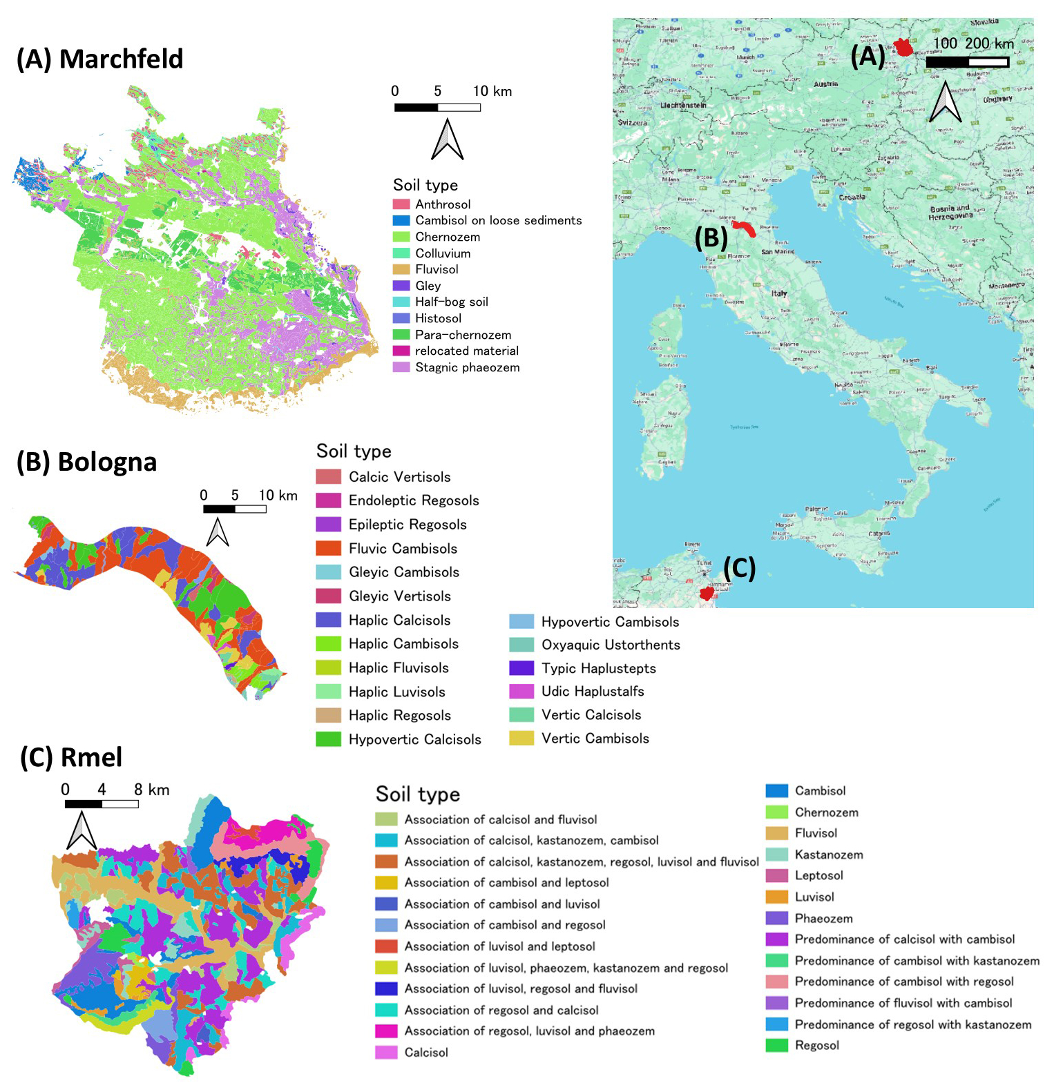
Figure 2 Marchfeld Region, Austria (A) (Fusco et al., 2024); Bologna, North-Italy (B) (ARPAE Emilia-Romagna, Soil maps from WebGIS portal: https://servizimoka.regione.emilia-romagna.it/mokaApp/apps/ped/index.html, last access: 2 November 2024); Rmel, Tunisia (C) (LANDSUPPORT: https://www.landsupport.eu/dss-platform/, last access: 8 November 2024, IAO, 2004); and the entire study areas map on the upper right corner (Map data © 2024 Google).

2.2 The FLOWS model

In the FLOWS model, the one-dimensional vertical transient water flow is simulated by numerically solving the Richards equation, using an implicit backward finite difference scheme with explicit linearization (Coppola et al., 2024; Hassan et al., 2024; Coppola et al., 2025) (Eq. 1):

$$\begin{array}{}\text{(1)}& C\left(h\right){\displaystyle \frac{\partial h}{\partial t}}={\displaystyle \frac{\partial }{\partial z}}\left(k\left(h\right){\displaystyle \frac{\partial h}{\partial z}}-k\left(h\right)\right)-S_{\mathrm{w}}\left(h\right)\end{array}$$

where C(h)= dθ $/$ dh [L⁻¹] is the soil water capacity, θ [−] is the volumetric water content, h [L] is the soil water pressure head, t [T] is time, z [L] is the vertical coordinate being positive upward, and K(h) [L T⁻¹] the hydraulic conductivity. The term S_w(h) [T⁻¹] is introduced for taking into account root water uptake.

The model discretizes the spatial flow field in a prescribed number of nodes (usually 100) of constant width (Δz). Time discretization starts with a prescribed initial time increment (Δt). This time increment is automatically adjusted at each time level according to the criteria proposed by Vogel (1987).

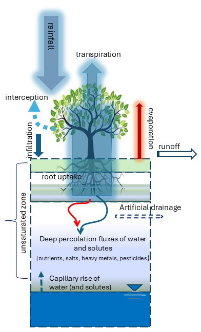
Figure 3 illustrates the overall schematic representation of water flow and solute transport processes simulated by the FLOWS model. The model has been used for several years in numerous studies addressing water and solute balances in stratified soil profiles, both at the theoretical level (e.g., Coppola et al., 2009, 2012, 2015b) and at the applicative levels (e.g., Wang et al., 2013; Coppola et al., 2015a, 2019a, b; Hassan et al., 2024; Porru et al., 2024). In addition, a variance-based sensitivity analysis was conducted for a structured bimodal soil, revealing that the variance of simulated water content is particularly sensitive to variability in the total macropore space fraction and, to a lesser extent, to the parameters n, α, K₀, τ (Coppola et al., 2009).

Figure 3 Water flow and solute transport processes simulated by FLOWS.

2.2.1 Hydraulic properties

Richards’ equation requires the water retention function, θ(h), and the hydraulic conductivity, K(h), function to be known. These functions interrelate pressure head, h, water content, θ, and hydraulic conductivity, K. Several water retention and hydraulic conductivity functions can be selected in the model, for these simulations we assumed the van Genuchten-Mualem (VGM) equations (Van Genuchten, 1980):

$$\begin{array}{}\text{(2)}& {\displaystyle }{S}_{\mathrm{e}}={\displaystyle \frac{\mathit{\theta }-{\mathit{\theta }}_{\mathrm{r}}}{{\mathit{\theta }}_{\mathrm{s}}-{\mathit{\theta }}_{\mathrm{r}}}}=[\mathrm{1}+|\mathit{\alpha }h{|}^n{]}^{-m}\text{(3)}& {\displaystyle }K\left(\mathit{\theta }\right)=K_{\mathrm{S}}{S}_{\mathrm{e}}^{\mathit{\tau }}{\left[\mathrm{1}-{\left(\mathrm{1}-S_{\mathrm{e}}^{\mathrm{1}/m}\right)}^m\right]}^{\mathrm{2}}\end{array}$$

where S_e is effective saturation, h [L] is the pressure head, α [L⁻¹] is related to the inverse of the air entry pressure head, n [−] and m [−] are shape parameters, with the constrain that m= $\mathrm{1}-\mathrm{1}/n$, θ, θ_r [−] and θ_s [−] are the actual, the residual and the saturated water contents, respectively, K(θ) [L T⁻¹] is the hydraulic conductivity function, K_S [L T⁻¹] is the hydraulic conductivity at θ=θ_s and τ is a parameter which accounts for the dependence of the tortuosity and the correlation factors on the water content.

2.2.2 Boundary and initial conditions for water flow

Flow rates and pressure heads, either constant or time-variable, can be used as the upper boundary condition. Similarly, gradients, pressure heads, or flow rates, whether constant or variable, can be applied at the bottom of the soil profile. In our simulations, daily flow rates (i.e., rainfall and potential evapotranspiration) were implemented as top boundary conditions. The reference evapotranspiration (ET₀) was estimated by applying the Hargreaves formula (Hargreaves and Allen, 2003), while the potential crop evapotranspiration (ET_p) is calculated as ET${}_{\mathrm{p}}=K_{\mathrm{c}}\cdot {\mathrm{ET}}_{\mathrm{0}}$, where K_c is the crop coefficient that varies with crop type, growth stage (Allen et al., 1998).

A fixed unit gradient (d$h/\mathrm{d}z=-\mathrm{1}$) was set as the bottom boundary condition for each soil profile, at the depth specific to the profile used in the simulations. Finally, the initial conditions can be set as either pressure head or water content, which may be constant or vary with soil depth. In this specific case, a constant pressure head condition was imposed, as reported in Table B1.

2.2.3 Vegetation processes and parameters

The vegetation is simulated in a so-called static way, so the growth of the crop is not dynamically simulated by the model, but the user has to specify the stage of crop development by providing as input the evolution over time of the leaf area index, root depth, and crop coefficient as a function of the stage of development.

The model applies Beer's law (Ritchie, 1972) to separate potential evaporation and transpiration from potential evapotranspiration, as given by the equation $E_{\mathrm{p}}={\mathrm{ET}}_{\mathrm{p}}\cdot \exp (-K_{\mathrm{l}}\cdot \mathrm{LAI}$). This requires the crop-specific light extinction coefficient (K_l) and the Leaf Area Index (LAI). To compute the actual evaporation, E_a, FLOWS calculates the maximum upward flux at the soil surface, E_max, allowed given the difference of atmospheric pressure, h_atm (in cm of water column) and the pressure head in the first simulation node, h₁, as:

$$\begin{array}{}\text{(4)}& E_{\max }=-K_{\mathrm{m},\max }\left({\displaystyle \frac{h_{\mathrm{atm}}-h_{\mathrm{1}}}{\mathrm{\Delta }{z}_{\mathrm{top}}}}-\mathrm{1}\right)\end{array}$$

where K_m,max is the arithmetic mean between the surface and top node hydraulic conductivities. In the case of E_p $<=$ E_max, E_a=E_p, else E_a = E_max. For further details the interested reader can refer to Coppola et al. (2025).

The integral over the rooted depth of the root water sink term, (S_w(h)), in Eq. (1) corresponds to the actual transpiration. S_w(h) is calculated in FLOWS according to a so-called macroscopic approach, frequently adopted in hydrologically oriented soil-plant-atmosphere continuum models for describing plant water uptake. According to the approach of Feddes et al. (1978), and neglecting the osmotic stress, it is calculated by the Eq. (5):

$$\begin{array}{}\text{(5)}& S_{\mathrm{w}}\left(h\right)=\mathit{\alpha }\left(h\right)S_{\mathrm{p}}\end{array}$$

where α(h) is the crop-specific water reduction function that depends on the local water pressure head at a given depth (z) and S_p is the potential root uptake, assumed to be equal to the potential transpiration. The function α(h) is a piecewise linear function that represents a reduction factor for root water uptake (ranging from 0 to 1), with five stages of water uptake defined by four values of pressure head (h₁ > h₂ > h₃ > h₄). The model accounts for different root distribution shapes with depth; in our study we applied the uniform root distribution function.

2.3 Input dataset for model simulations

• Climate. For each case study, we first analyzed the variability of long-term climatic data, considering both annual rainfall totals and intra-annual rainfall distribution, alongside reference ET. Subsequently, a representative median climatic year was selected for each case study. The selected year corresponds to the one within the full observation period whose annual rainfall and then ET were closest to the median of the long-term dataset at each site. This approach ensures that the chosen year reflects typical rainfall and evapotranspiration conditions, making it representative of the site’s median hydro-climatic regime. This choice served two main objectives: (i) to generalize the model results, ensuring that they are representative of the investigated areas, and (ii) to reduce the computational demand associated with solving the Richards equation.

  The representative median year for the Marchfeld site, within the period from 1997 to 2016, was identified as the year spanning from October 2006 to September 2007, with an annual rainfall of 526 mm and a reference evapotranspiration of 952 mm. This year exhibited rainfall closest to the median value calculated for the 20-year dataset, making it a typical representation of the region's average rainfall pattern. For Bologna, the representative median year during the period from 1991 to 2022 was identified as the year spanning from October 2017 to September 2018, with an annual rainfall of 746 mm and a reference evapotranspiration of 1106 mm. This year closely matched the median rainfall value calculated for the 32-year dataset, reflecting typical rainfall conditions for the region. For Rmel, the representative median rainfall year during the period from 2008 to 2018 was identified as the year spanning from October 2009 to September 2010, with an annual rainfall of 410 mm and a reference evapotranspiration of 1193 mm. This year corresponds to the median value of the dataset, representing typical rainfall conditions for the region during the study period.

  Model simulations were conducted using a daily time step. This temporal resolution may, in some cases, limit the explicit simulation of surface runoff processes generated by short-duration, high-intensity rainfall events. However, the primary objective of this work was centered on simulating the daily soil–water balance and to provide baseline information on climate–soil interactions, with a specific focus on infiltration, evapotranspiration, and soil moisture dynamics, rather than event-based runoff generation. Furthermore, the selection of the daily time step is justified by the limited availability of high-frequency data across the large spatial scale encompassing the three case studies.

• Soil. Each soil profile was discretized into multiple horizons based on the available site data, resulting in a total of 315 soil profiles and 965 soil horizons across the three study areas. The data on soil texture and organic matter content were available for each horizon of the investigated soil profiles. For each horizon, these data were used as inputs in the pedotransfer functions to predict bulk density [g cm⁻³] (Hollis et al., 2012) and soil hydraulic properties (θ_s [−], α [cm⁻¹], n [−], K_S [cm d⁻¹] and τ [−]) (Wösten et al., 1999).

  The available water content (AWC) was computed as the difference between soil water content at field capacity and at the permanent wilting point (AWC $={\mathit{\theta }}_{\mathrm{FC}}-{\mathit{\theta }}_{\mathrm{WP}}$).

  It is important to stress that the K_S used in our simulations does not represent field-saturated conductivity ($K_{{\mathrm{S}}_{\mathrm{f}}}$): given the 315 soil profiles analysed, consistent data on macropore presence and parametrization were not feasible. Thus, the focus was on matrix conductivity, while acknowledging that macropore flow is important at the local scale.

  To complement the indicators already presented, we introduced an additional metric that estimates the nature and extent of macroporosity, calculated as the difference between θ_s and field capacity. This approach, inspired by the conceptual framework proposed in Hirmas et al. (2018), provides a practical means of inferring the potential for preferential flow pathways within the soil matrix. This addition enhances the comprehensiveness of our discussion and allows us to better address the complexity of water movement in structured soils.

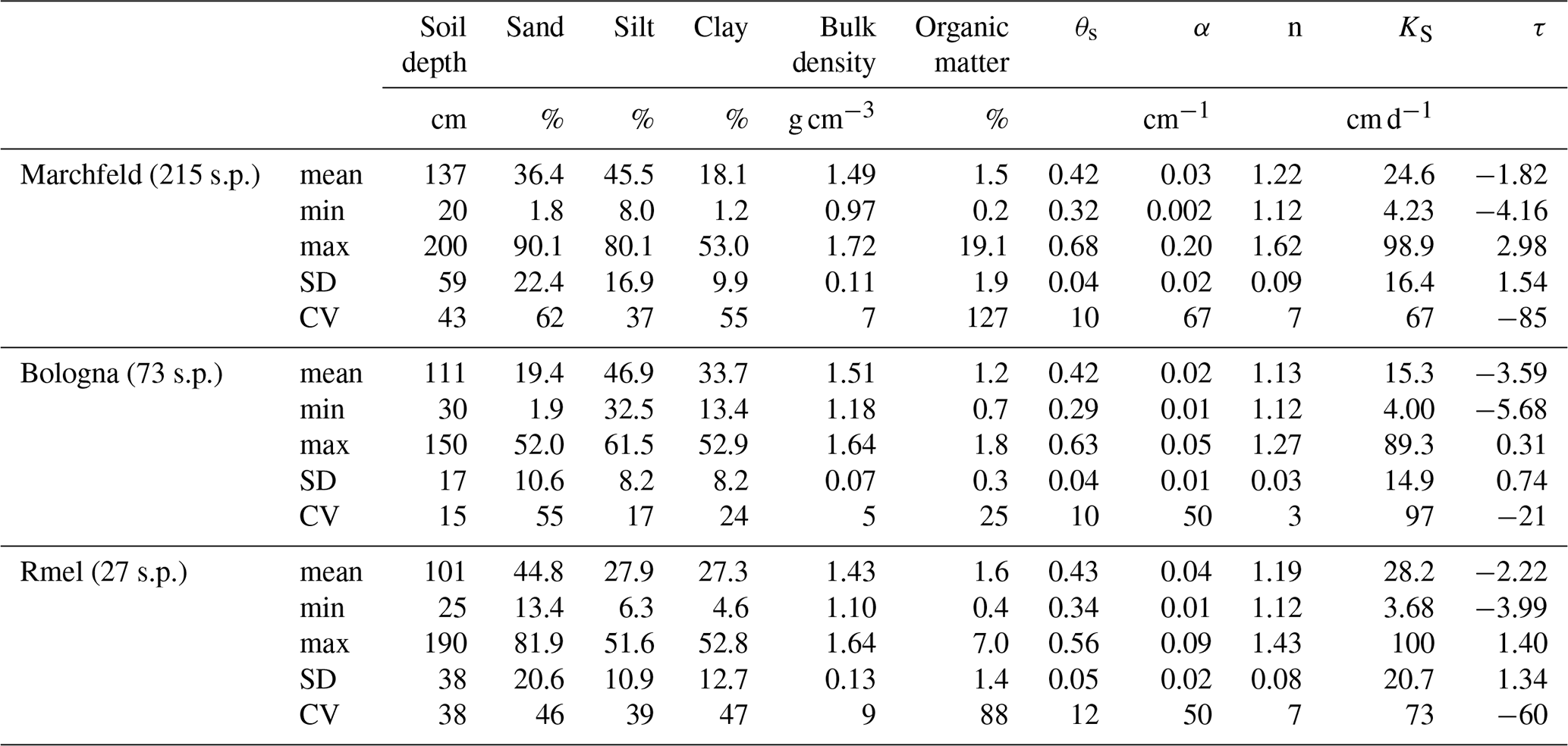
  Finally, we computed (i) the weighted mean of these properties over the horizon depths, and (ii) the arithmetic mean across all soil profiles within each site, in order to obtain overall descriptive statistics shown in Table 1.

• Crop. The vegetation module of the FLOWS model was parameterised specifically for durum wheat (Triticum turgidum subsp. durum) largely cultivated at the three sites. Moreover, the absence of irrigation simplifies the analysis by reducing variability due to water management, making it a suitable reference case for our assessment framework. The light extinction coefficient was set to K_l= 0.45. The crop development stages were determined by integrating the FAO56 guidelines with expert knowledge, literature, and site-specific field observations. This approach ensured a robust and site-appropriate parameterization of crop development for each case study. Compared to the typical crop calendar and the growth stages described in FAO56, flowering occurs earlier at Rmel than at Marchfeld and Bologna; while sowing takes place earlier at Marchfeld and Bologna compared to the Rmel site. The crop coefficient (K_c), was derived accordingly and integrated with values taken from the literature (Allen et al., 1998). The Leaf Area Index (LAI) was modeled using Growing Degree Days (GDD), applying a lognormal function (Campbell and Norman, 1998). The water stress coefficients h₁–h₄ of the Feddes model were set as crop specific as follows: h₁ = −1 cm, h₂= −10 cm, $h_{\mathrm{3}}^{\mathrm{H}}=$ −400 cm, $h_{\mathrm{3}}^{\mathrm{L}}=$ −800 cm, h₄= −8000 cm, where the superscripts H and L for the H3 values refer to high (5 mm d⁻¹) and low (1 mm d⁻¹) potential evapotranspiration, respectively. Finally, the maximum rooting depth for durum wheat was set to 60 cm, with a uniform root distribution function.

Table 1 Mean, minimum, maximum, standard deviation (SD) and coefficient of variation (CV) of the main soil characteristics of input dataset in the study areas of Marchfeld, Bologna and Rmel. The number of investigate soil profile (s.p.) is reported in parenthesis for each site.

2.4 Ecosystem Services and Indicators

Water-related processes within the soil-plant-atmosphere system, such as infiltration, evapotranspiration, and groundwater recharge, are integral components of the hydrological cycle. These processes are primarily influenced by climate and soil hydrological properties. By simulating these processes, the FLOWS model provides outputs that enable the estimation of four key regulating ecosystem services:

• Runoff triggering (RUN). the contribution of the soil in separating the amount of water that infiltrates from the portion that flows externally, potentially generating flux-to-runoff.

• Infiltration (INF). the soil's ability to regulate water entry, contributing to water regulation services.

• Groundwater recharge (GWR). the soil's capacity to conduct water downward and replenish groundwater, thereby supporting water regulation services. Irrespective of soil thickness or groundwater table depth (if the groundwater does not intersect the soil profile), GWR decribes the outflow from the profile. In terms of ecosystem services, this flux corresponds to potential groundwater recharge.

• In addition, the Crop Water Stress Index (CWSI) is considered a proxy indicator for food provision ecosystem services, measuring the level of water stress experienced by crops. CWSI is calculated as (1 $-T_{\mathrm{act}}/T_{\mathrm{pot}}$) ⋅ 100, where T_act is actual transpiration and T_pot is potential transpiration.

These outputs were analysed to evaluate their interrelations with a group of key soil parameters which are commonly selected as indicators of water regulation ecosystem services. These indicators encompass saturated hydraulic conductivity (K_S), available water content (AWC), bulk density (BD), organic matter (OM), clay content (CLAY), saturated soil water content (θ_s), macroporosity (MACRO), and soil depth (SD).

2.5 Statistical analysis

Various descriptive analysis tools and summary measures were used to explore and describe the data, as well as to visualize their distributions. To investigate the degree of correlation between ecosystem services and indicators (soil properties), we performed the simple linear regression and calculated the Pearson correlation using the metan package in R software (Olivoto and Barbin, 2020). In the text, we classify the degree of correlation (r) as follows: very weak (< 0.2), weak (0.2–0.4), moderate (0.4–0.6), strong (0.6–0.8), and very strong (> 0.8). Scatter-plots were generated using the AgroR package (Shimizu et al., 2022) and the ggplot2 package (Wickham, 2016) in R.

In addition, stepwise multiple linear regression analyses were performed to identify linear relationships between selected ecosystem services and soil properties, utilizing the olsrr package in R (Hebbali, 2020). The stepwise selection method applied p-values to determine the most parsimonious model. The statistical significance of model parameters was assessed by performing an analysis of deviance (validated by F-tests) to compare a null model (no effect) with models that included one or more explanatory variables.

All statistical analyses and graphing were conducted using RStudio software, version 4.3.2 (R Core Team, 2023).

3 Results

This section is organized into four subsections to present the findings of the analysis across all three case study areas.

• Section 3.1 discusses the contribution of each individual process on the overall soil water balance, providing insights into how processes like infiltration, evaporation, plant uptake, and groundwater recharge contribute in each region.

• Section 3.2 analyses the soil data used in the simulations, highlighting the study area's diverse pedological characteristics. These data encompass critical physical and hydrological properties essential for modelling water-related processes in the soil-plant-atmosphere continuum.

• Section 3.3 evaluates the simple bivariate relationships between individual soil indicators (e.g., saturated hydraulic conductivity, bulk density, and organic matter content) and each water-related process. This analysis aims to determine how well specific indicators can predict or represent particular processes.

• Section 3.4 explores the multivariate relationships between indicators and their influence on each water-related process. By examining these interactions, this analysis seeks to understand potential synergistic or antagonistic effects of indicator combinations on infiltration, groundwater recharge, and crop water stress index.

Each subsection provides detailed insights into the functioning and inter-dependencies of soil indicators and water processes, contributing to a comprehensive understanding of soil-water interactions in different environmental settings.

3.1 Overview on the water balance components

The overall results of the simulated water balance components, including interception, infiltration, flux-to-runoff triggering, transpiration, evaporation, and groundwater recharge are presented in Table 2. These processes are described through their mean, minimum, and maximum values, as well as through their ratio to rainfall, in order to synthetize the behaviour of each area.

Table 2 Mean values (with coefficient of variation, %), minimum, maximum and relative contributions of the different components of the water balance are reported: interception, flux-to-runoff, and infiltration are expressed as percentages of rainfall; transpiration, evaporation, and groundwater recharge are expressed as percentages of infiltration. CWSI refers to crop water stress index (%). Annual values are presented for each component across the study areas of Marchfeld, Bologna, and Rmel.

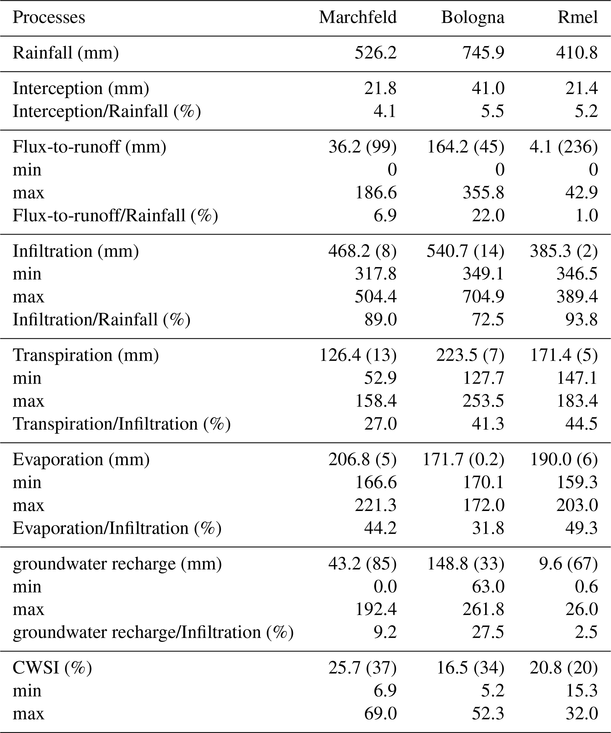
Overall, the terms of the water balance in the three study regions of Marchfeld, Bologna, and Rmel revealed significant differences, driven primarily by differences in the amounts of rainfall (Table 2) and the annual distributions. In fact, Bologna received the highest annual rainfall (746 mm), followed by Marchfeld (526 mm), and Rmel (411 mm), characterized by the lowest rainfall amount. A focus on the annual distributions of each case study is given in Appendix A1.

Mean interception losses were consistently low, ranging from 21.4 to 41.0 mm across the regions, indicating that canopy cover has a relatively small effect on the total water budget.

The mean surface flux-to-runoff in Bologna was significant (164.2 mm), primarily due to the texture of the dominant soils in the area, which range from fine silty to silty clay loam. This soil texture is associated with low K_S, resulting in the activation of overland flow when rainfall exceeds the soil’s infiltration capacity (Beven, 2004). The importance of this mechanism is evidenced by historical and recent flooding disasters in the Emilia-Romagna region (Arrighi and Domeneghetti, 2024). In contrast, Rmel exhibited negligible flux-to-runoff (4.1 mm), which can be attributed to its low rainfall levels and rates, as well as its coarser soils. These soil characteristics enhance infiltration capacity, reducing surface flux-to-runoff.

The infiltration of net rainfall – defined as total rainfall minus flux-to-runoff and vegetation interception – accounts for a large fraction of total rainfall in Rmel (385.3 mm; ∼ 90 %) and Marchfeld (468.2 mm; ∼ 90 %). In contrast, despite higher absolute rainfall amounts, infiltration in Bologna (540.7 mm) represents a smaller fraction of total rainfall (∼ 73 %), primarily due to higher flux-to-runoff losses.

Mean crop transpiration was higher in Bologna (223.5 mm) compared to Rmel (171.4 mm) and Marchfeld (126.4 mm). The latter exhibited the lowest values, primarily due to the lower temperatures compared to Bologna and Rmel. The mean evaporation is similar across the three case studies (around 190 mm).

The average amount of water leaving the soil profile (i.e., groundwater recharge) was notably higher in Bologna (148.8 mm). This was primarily due to the significant rainfall levels, but also to the relative homogeneity of the soil horizons, which facilitate water flow. Indeed, it is well known that the greater the heterogeneity along the soil profile, the lower the water flow through these horizons (Matthews et al., 2004). In contrast, Rmel exhibited the lowest mean groundwater recharge (9.6 mm), likely due to the limited rainfall. The relatively low amount of rainfall and the high variability of soils in Marchfeld result in intermediate values for infiltration, flux-to-runoff triggering, and groundwater recharge, falling between those observed in Bologna and Rmel.

Eventually, the total change in soil water storage was computed over the assessed simulation period and integrated over the soil profile down to the locally defined maximum soil depth for each soil in each site. Under these conditions, the average simulated water storage change was higher in Marchfeld (91.8 mm) than in Rmel (14.4 mm) and Bologna (−3.3 mm). These values should be interpreted in the context of site-specific soil depth and initial conditions. In particular, the larger storage change in Marchfeld is mainly associated with its greater effective soil depth and right-skewed depth distribution (Table 1), which promote the retention of infiltrated water within the soil profile. Conversely, the negative storage change simulated for Bologna reflects its lower soil depths and related variability. Changes in soil water storage are sensitive to initial soil moisture conditions; accordingly, the reported values represent relative changes over the assessment period rather than long-term equilibrated states.

3.2 Analysis of the soil profiles dataset

A summary of the primary soil characteristics and hydraulic properties observed in the three study regions is given in Table 1. Variability in soil depth across the study areas reflects regional differences in soil profiles, which have significant implications for water-related processes such as infiltration and groundwater recharge. On average, Marchfeld exhibit deeper soil profiles (approximately 137 cm) compared to Bologna and Rmel, where the average soil depth is about 111 and 101 cm, respectively. Marchfeld exhibits the largest variability in soil depth, with a coefficient of variation (CV) of 43 %, followed by Rmel (CV = 38 %) and Bologna (CV = 15 %).

The soils of Bologna are predominantly heavy, with clay and silt making up over 80 % of the composition. This suggests a predominance of fine particles, which typically results in slower infiltration rates and higher water retention, as discussed previously. Furthermore, the Bologna area exhibits the lowest variability in texture, with coefficients of variation (CV) for silt at 17 % and clay at 24 %. This limited variability suggests a more homogeneous soil texture, which is likely to result in relatively uniform soil hydraulic properties and a more spatially consistent hydrological behaviour, potentially reducing uncertainty in model simulations at the regional scale.

Soils in Rmel are different from the above cases, with a higher sand content averaging 45 %. Sandy soils generally facilitate faster infiltration and lower water retention. However, the variability in texture is considerably higher in Rmel, with CV values for silt and clay ranging between 39 % and 47 %. This heterogeneity may contribute to more variable water-related processes and localized differences in soil behaviour. Texture variability in Marchfeld falls between that of Bologna and Rmel, with CV values also ranging in between the other two sites. This suggests a diverse soil structure, potentially leading to spatial differences in water movement and storage.

Variability in soil texture among the three study areas corresponds to significant differences in their hydraulic properties. The mean values of key soil hydraulic parameters – namely, saturated water content (θ_s), air-entry parameter (α), shape parameter (n), saturated hydraulic conductivity (K_s), and the pore connectivity/tortuosity factor (τ) – differed statistically significantly between the areas. The mean values and coefficients of variation of (θ_s) and α remain similar across the three areas. More pronounced differences are observed in the parameters n and K_s, both of which are critical for governing water flow in the soil. Higher values of n indicate steeper water retention curves, which imply greater and faster water release from the soil as matric potential decreases. Higher values of K_S signify faster water movement through the soil profile. These variations reflect the influence of texture, with coarser soils (e.g., Rmel) generally exhibiting higher K_S (28 cm d⁻¹) values, allowing quicker infiltration and groundwater recharge, while finer soils (e.g., Bologna) tend to have lower (15 cm d⁻¹), retaining water for longer periods. As expected, the coefficients of variation (CVs) of K_S are notably high across the three study areas, reflecting the inherent variability of this property: Bologna CV = 97 %, Rmel CV = 73 % and Marchfeld CV = 67 %.

The stark contrast between the heavy, homogeneous soils of Bologna and the coarser, heterogeneous soils of Rmel underlines the importance of site-specific soil management strategies and response to climatic inputs.

As an example on how different soil types influence water partitioning processes, the pie chart in Fig. 4 illustrates the distribution of infiltrated water among transpiration, evaporation, and groundwater recharge for three distinct soil types in the Marchfeld region, which displays the highest variability among the three study areas. These soils exhibit markedly different characteristics: the Para-chernozem is shallow (< 50 cm), with a high sand content (> 60 %); the Fluvisol is considerably deeper (130 cm), characterized by a silty texture and a high organic matter content (OM = 4.6 %); and the Stagnic Phaeozem is the deepest (200 cm), with an organic matter content of 2.7 %.

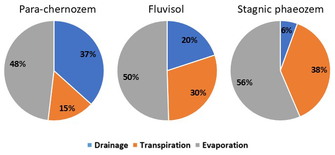
Figure 4 Percentage of infiltrated water distributed among three processes – transpiration, evaporation, and groundwater recharge – in the Marchfeld region for soil profiles Para-chernozem, Fluvisol, and Stagnic phaeozem.

The contribution of evaporation is nearly identical across the different soil types, with 48 % for para-chernozem, 50 % for Fluvisol, and 56 % for stagnic phaeozem. This consistency suggests that evaporation is primarily driven by atmospheric demand. As the initial phase of the evaporation process is weather-controlled (Pearse et al., 1949), the soil’s role in the process itself remains minimal, especially given the temporal distribution of rainfall.

This holds true for all the investigated sites, where the variability of the evaporation amounts among the investigated soils is low (the coefficient of variation ranges from 0.2 % to 6 %).

The percentage contribution of transpiration increases from Para-chernozem to Fluvisol and then to Stagnic Phaeozem, while groundwater recharge follows an inverse pattern. This behavior is predominantly controlled by variations in the pore size distribution both along individual soil profiles and among different soil types, which is reflected in their distinct hydraulic properties. For example, in Stagnic Phaeozem soil, the presence of a fine-textured subsurface horizon significantly impedes water movement through the soil profile, resulting in reduced groundwater recharge efficiency compared to Fluvisol and Para-chernozem. Consequently, Stagnic Phaeozem exhibits prolonged water retention, thus enhancing the availability of soil moisture for evapotranspiration over an extended period.

A further example highlighting the importance of applying a modelling approach to disentangle soil hydrological complexity is provided by assessing the effects of parameter changes – specifically, an increase in bulk density associated with tillage – on soil layering, whose resulting water dynamics cannot be predicted a priori. Figure 5 presents a comparison of three soils from the Marchfeld, Bologna, and Rmel regions that share similar texture (Silty Clay Loam), comparable hydraulic properties, a total soil depth of 80 cm, and an Ap horizon depth of 30 cm. For each soil, the main components of the water balance – groundwater recharge, flux-to-runoff, and transpiration – were simulated under three different climatic conditions, both in the absence of soil compaction (solid bars) and with the presence of a 10 cm-thick plow pan at 20 cm depth (shaded bars). The plow pan was represented by increasing bulk density by 20 % within the 20–30 cm soil layer of each soil.

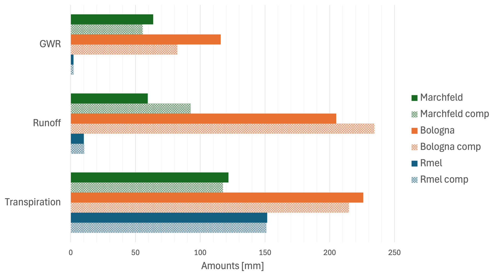
Figure 5 Simulated water balance components for three Silty Clay Loam soils under different climatic conditions, without (solid bars) and with a plow pan at 20–30 cm depth (shaded bars), represented by a 20 % increase in bulk density.

Overall, the figure highlights how climatic conditions exert a dominant control on the partitioning of the water balance, while soil physical constraints, such as the presence of a plow pan, modulate water fluxes in different ways depending on climate. Under the Marchfeld climate, water losses are mainly driven by transpiration, with limited runoff generation. The introduction of a plow pan slightly reduces groundwater recharge (−13 %, from 64 to 56 mm) and transpiration (−3%, from 122 to 118 mm), while increasing surface runoff (+56 %, from 59 to 93 mm), indicating a reduced vertical percolation capacity and a stronger surface response. In the Bologna case study, characterized by higher precipitation amounts, runoff becomes a major component of the water balance, particularly when the plow pan is present. The simulated plow pan leads to a marked increase in runoff (+14 %, from 205 to 235 mm) and a corresponding reduction in groundwater recharge (−29 %, from 116 to 82 mm), highlighting the strong interaction between soil compaction and wetter climatic conditions. Transpiration remains high (−5 %, from 226 to 214 mm), but their relative contribution is less dominant compared to runoff. For the RMEL climate, representative of semi-arid conditions, the water balance is largely controlled by transpiration, with negligible groundwater recharge and runoff. The presence of a plow pan has only a marginal effect on most components (+3 % of increasing for both GWR and runoff, from 2 to 2.1 mm and from 10 to 10.3 mm, respectively), reflecting the limited role of soil hydraulic constraints under water-limited conditions. Overall, the comparison demonstrates that the impact of soil compaction on water balance components is strongly climate-dependent, with the most pronounced effects occurring under humid conditions, intermediate effects under temperate climates, and minimal influence in semi-arid environments. No relevant differences were observed in evaporation and interception between the compacted and non-compacted scenarios.

3.3 Interrelationship between soil indicators and ecosystem services

The Pearson correlation coefficients (r) between the seven soil indicators (K_S, AWC, BD, OM, CLAY, θ_S, and SD) and the four ecosystem services (RUN, INF, GWR, and CWSI) for Marchfeld, Bologna, and Rmel are summarized in Table 3. Asterisks denote significance levels: (^*) for (p<0.05), (${}^{**}$) for (p<0.01), and (${}^{***}$) for (p<0.001). These levels indicate varying degrees of statistical significance, with lower p-values showing stronger evidence against the null hypothesis.

Table 3 Pearson correlation coefficients (r) between process of soil water balance and soil properties in Marchfeld, Bologna and Rmel. (INF = infiltration; GWR = groundwater recharge; RUN = flux-to-runoff; CWSI = crop water stress index (%); SD = soil depth; OM = organic matter; BD = bulk density; θ_s = saturated water content; K_s = saturated hydraulic conductivity; AWC = available water content; MACRO = macro-porosity.

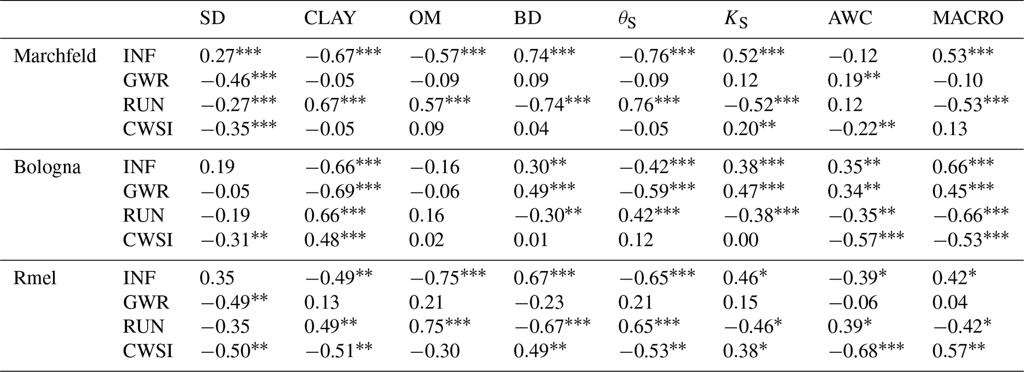
Note: Asterisks denote significance level (^* p<0.05; ${}^{**}$ p<0.01; ${}^{***}$ p<0.001).

Soil depth (SD) shows moderate to weak correlations (from $r=\left|\mathrm{0.19}\right|$ up to $r=\left|\mathrm{0.50}\right|$) across the three sites, except for GWR in Bologna, where the correlation is nil (r= −0.05). Firstly, it is worth noting that the correlations for RUN show the same value as INF. This holds for all the investigated parameters because the amount of infiltrated water is directly calculated as the difference between rainfall (which is constant for each area) and flux-to-runoff. Therefore, the correlation coefficient is the same but with the opposite sign. In particular, INF/RUN showed weak correlations with SD (from $r=\left|\mathrm{0.19}\right|$ up to $r=\left|\mathrm{0.35}\right|$), and a moderate negative correlation with GWR (r= −0.46 and r= −0.49 for Marchfeld and Rmel, respectively). These correlations are negative, as expected: the deeper the soil, the lower the flux of water below the soil bottom, and consequently, the lower the GWR. Finally, for CWSI, the correlation ranges from weak (r= −0.31) to moderate (r= −0.50), with negative values since deeper soils are associated with reduced crop stress.

Clay content (CLAY) exhibits the highest values among the seven indicators. INF is strongly negatively correlated in Marchfeld (r= −0.67) and Bologna (r= −0.66) and moderately negatively correlated in Rmel (r= −0.49). GWR shows a higher negative correlation only in Bologna (r= −0.69), while CWSI exhibits a moderate correlation in both Bologna and Rmel. However, the correlation coefficients have opposite signs: in Bologna, higher clay content is associated with increased stress, whereas in Rmel, clay content appears to reduce stress. This contrasting behavior in Rmel could be explained by its predominantly sandy soils, where an increase in clay acts as a structuring factor, enhancing soil water retention capacity and thereby reducing crop water stress.

Organic matter (OM) is negatively correlated with infiltration in Marchfeld (moderate, r= −0.57) and Rmel (strong, r= −0.75). All other correlations between organic matter and processes are weak.

Bulk density (BD) of the upper layer is strongly positively correlated with INF in the Marchfeld (r=0.74) and Rmel (r=0.67) case studies, showing a high level of significance (p<0.001). In contrast, bulk density in Bologna exhibits only a weak linear correlation with infiltration. Positive correlation between BD and K_S likely reflects site-specific soil structural conditions and potential multicollinearity among soil physical properties. This relationship is most pronounced in Rmel (r=0.49, p<0.01), followed by Bologna (r=0.30, p<0.05), while it is comparatively weak but still statistically significant in Marchfeld (r=0.14, p<0.05). An analysis of the processes reveals that high bulk density values correspond to high sand content, which, on the one hand, reduces porosity but, on the other, increases K_S, primarily enhancing infiltration. As a result, positive correlations are observed. No clear pattern is observed for GWR and CWSI, although a moderate positive correlation is found for GWR at the Bologna site and for CWSI at the Rmel site.

Saturated soil water content (θ_S) exhibits a strong negative correlation with infiltration at the Marchfeld (r= −0.76) and Rmel (r= −0.65) sites, while in Bologna, the correlation is moderately negative (r= −0.42). A moderate negative correlation is also observed for GWR at the Bologna site and for CWSI at the Rmel site. The behavior of θ_S follows a similar correlation pattern to bulk density (BD) but with the opposite sign. This is expected, as the two indicators are closely related, given that θ_S is assumed to be equal to soil porosity.

Saturated hydraulic conductivity (K_S), despite being considered the best indicator for infiltration, shows a moderate positive correlation in Marchfeld (r=0.52) and Rmel (r=0.46) and a weak correlation in Bologna. The moderate positive correlation with GWR in Bologna (r=0.47) suggests that, due to the reduced permeability of the entire profile, higher K_S values in the upper horizon lead to increased groundwater recharge at the bottom of the soil profile. PTFs often lead to a reduction in the variability of hydrological properties, particularly K_S. This effect arises because PTFs estimate K_S based on more readily available soil properties, such as texture, bulk density, and organic matter content, using empirical relationships or statistical models.

Available water content (AWC) with regard to INF, GWR and RUN, moderate to weak correlations were observed, with values ranging from −0.12 up to 0.39. Furthermore, in the case of INF, it is evident that the correlation in Bologna is weak and postive, whereas in Rmel it is weak but negative. This suggests that there is no consistent physical relationship between AWC and infiltration. Therefore, regardless of climate or soil type, the use of this indicator is not recommended for representing the ecosystem service of infiltration.

AWC shows a moderate correlation with CWSI in Bologna (r= −0.57) and a strong correlation in Rmel (r= −0.68), whereas a weaker correlation is observed in Marchfeld (r= −0.22). This variation in behaviour among the three sites can be attributed to differences in rainfall distribution. In Bologna and Rmel, the higher soil water storage capacity (higher AWC) allows intermittent rainfall to be effectively stored in the soil, thereby reducing crop water stress. In contrast, the more consistent rainfall distribution in Marchfeld prevents the onset of water stress, reducing the significance of soil water storage capacity in this region. Additionally, this steady rainfall pattern minimizes runoff, allowing most of the rainfall to infiltrate the soil and remain readily available for crop growth, regardless of the soil's storage capacity. Specifically, the soils in Marchfeld infiltrate 90 % of the rainfall, compared to only 73 % in Bologna, primarily due to Bologna’s higher flux-to-runoff (164.2 mm) relative to Marchfeld (36.2 mm).

3.4 Multivariate analysis of interrelations between soil indicators and ecosystem services

To deepen the analysis, we moved from a one-to-one single correlation between parameters and process to a multi-to-one regression approach. The fundamental principle of the stepwise regression procedure is to sequentially add or remove predictor variables from the model based on a p-value threshold of 0.05. This process continues iteratively until no further adjustments are statistically justified. Hence, in Table 4, the ranking of importance of the soil properties for each site and the four ecosystem services is provided, along with the correlation coefficient (r), the MAE and the corresponding p-value. A higher ranking indicates a greater contribution of the parameter to the process, thereby enhancing prediction accuracy.

Table 4 Statistics of multiple linear regression models predicting processes of soil water balance based on the interaction effect of soil properties in Marchfeld, Bologna and Rmel. (INF = infiltration; RUN = flux-to-runoff; GWR = groundwater recharge; CWSI = crop water stress index; OM = organic matter).

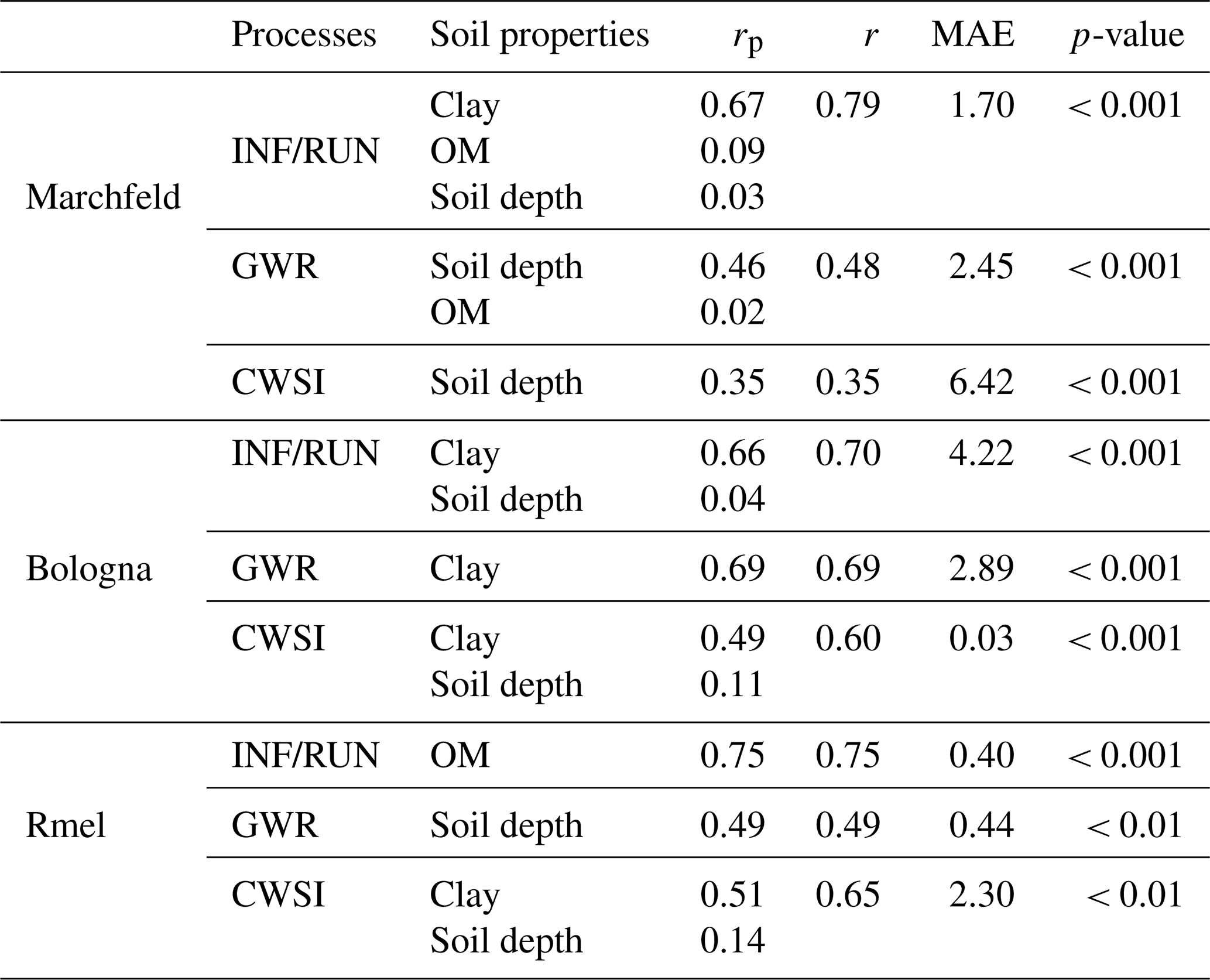
Note: MAE = Mean Absolute Error (cm); r_p= correlation between the individual soil properties and the model; r= overall correlation coefficient of the model.

The step-wise regression analysis included three variables (indicators): Soil depth, Clay content, and Organic matter content. The remaining four variables (θ_S, BD, K_S, and AWC) were excluded as they are dependent on the preceding ones. Specifically, BD, θ_S and K_S were derived from a pedotransfer function, which considers clay content and OM as input, among other parameters. Finally, AWC is also a function of soil depth.

In four out of nine possible cases, multiple regression did not yield any further improvement over simple linear regression. Specifically, in these cases – soil depth for CWSI in Marchfeld, clay content for GWR in Bologna, organic matter for INF/RUN and soil depth for GWR in Rmel – the correlation coefficient was already at its maximum compared to the other variables, meaning that the results remained unchanged.

In three of the remaining six cases, the combination of clay content and soil depth emerges as the best predictor, with clay content being negatively correlated and soil depth being positively correlated. Specifically, at the Bologna site, multiple regression with INF/RUN exhibits a strong correlation (r=0.70), with an average overestimation of approximately 4 cm. Additionally, the t-value for clay is around 8, whereas for soil depth, it is 2.8, indicating that clay shows three-times the level of confidence as a predictor. From a physical perspective, it is important then to highlight that these two variables do not contribute equally to the process. The Crop Water Stress Index (CWSI) is influenced by both clay content and Soil depth at the Bologna and Rmel sites. At the Bologna site, the correlation coefficient is moderate to strong (r=0.60), with the Mean Absolute Error (MAE) approaching zero. At the Rmel site, a strong correlation is observed (r=0.65) with an MAE of 2.3 cm. The t-values indicate greater significance for the clay content (5.3) compared to the depth of the soil (−3.7) in Bologna, while in Rmel similar t-values are observed (−2.6). Notably, despite the similar statistical metrics between Bologna and Rmel for CWSI, the variables impact the sites differently. At Rmel, both clay content and soil depth are negatively correlated with CWSI, suggesting that higher values of these variables correspond to reduced crop stress. In contrast, at Bologna, this negative correlation is observed for the only Soil depth variable. This discrepancy may be due to higher clay content leading to increased flux-to-runoff and reduced water infiltration, thereby decreasing soil water availability for root uptake.

4 Discussion and Conclusions

This study’s findings underscore the importance of understanding local soil and climatic variations to better manage water-related processes and ecosystem services. To this end, we treated each soil profile as independent and representative of a single soil map unit, allowing us to investigate the local variability of soil properties within each study area. While our modelling design focuses on unit-to-regional scale patterns rather than formal spatial upscaling, it effectively captures the heterogeneity in soil properties and provides insights into differences observed both within and across the three regions. The differences among the Marchfeld, Bologna and Rmel regions reveal how unique pedoclimatic conditions can shape hydrological behaviour and affect related ecosystem services. By examining these distinct regions, the study contributes valuable insights that could guide tailored approaches to soil and water management, ensuring more effective conservation and sustainable land use practices in various climatic zones. To achieve the objectives of this research, which aims to evaluate the effectiveness of widely proposed indicators based on soil properties in accurately representing water-related soil functions and processes. We also assess how well these indicators reflect the ecosystem services provided by soils in terms of water regulation. To this end, we systematically advance along the staircase scheme shown in Fig. 1. In this context, the results of this study can be discussed as follows:

• We propose that the effective evaluation of widely proposed soil-property-based indicators in accurately representing water-related soil functions should not be considered as a linear process. Instead, it may often require progressive refinement driven by site-specific conditions. In this regard, Fig. 1 could be more appropriately represented a cyclical process of refinement. During this loop, parameters could be added or discarded based on the unique characteristics of each site. This adaptive approach is particularly important given the complexity of climate–soil interactions. Accordingly, this study used a median climatic year to provide a baseline representation, recognizing that the refinement process would benefit from incorporating inter-annual climatic variability in future applications. It is also important to note that this analysis was conducted at a daily time step; however, for some water balance components, such as potential runoff generation, a finer temporal resolution would be more suitable. This is particularly relevant given the projected increase in high-intensity, short-duration rainfall events associated with climate change (Prein et al., 2017). Clearly, extending such analyses over longer time spans, under more extreme climatic conditions, and at finer (e.g., hourly) temporal resolution would provide additional and complementary insights.

• Some commonly used parameters did not show the expected correlation with the investigated processes, while others proved more relevant. These findings challenge conventional assumptions and highlight the need for context-specific indicator selection.

  A notable example is saturated hydraulic conductivity (K_S), which is often regarded as a key predictor of infiltration rates and water-regulation ecosystem services. However, in our case studies, K_S exhibited only moderately positive correlations with infiltration (r=0.52 in Marchfeld and r=0.46 in Rmel), and even weaker correlations in Bologna (r=0.38) – values lower than those for clay content, θ_s, and bulk density. This finding aligns with contradictory evidence reported in the literature. Coppola et al. (2009) found that soil structure played a dominant role in aggregated soils, concluding that K_S was not the most suitable indicator for capturing the effect of soil aggregation on hydraulic behaviour. In contrast, Baritz et al. (2023) selected K_S as the best indicator for soil compaction and related processes such as infiltration and flux-to-runoff in their review of soil health indicators. Similarly, Calzolari et al. (2016) used K_S as one of the indicators for water regulation ES, derived from locally calibrated PTFs. Reconciling these contrasting findings remains challenging, largely because of the substantial discrepancies reported between field-measured and laboratory-derived K_S values, which introduce considerable uncertainty into its use as a soil health indicator. These discrepancies are mainly attributable to incomplete soil saturation during field measurements (Basile et al., 2003), which can lead to differences in K_S of up to one to three orders of magnitude (Pachepsky et al., 2004). Additional uncertainty arises from the use of pedotransfer functions and from the presence or absence of preferential flow pathways, further complicating the interpretation of K_S-based assessments. From a soil health perspective, these uncertainties raise critical concerns regarding the use of K_S as a standalone indicator. Soil health frameworks increasingly emphasize indicators that are not only sensitive to soil functions but also robust, reproducible, and comparable across sites and measurement protocols. Given the limited standardization and high variability associated with K_S, its “blind” use to infer hydrological processes such as infiltration and runoff may lead to unreliable estimates of water-related ecosystem services. In contrast, other soil hydraulic indicators that exhibit greater stability and lower methodological uncertainty (e.g. saturated water content) are often more suitable for inclusion in soil health assessment frameworks, as they provide more consistent links between soil properties, hydrological functions, and ecosystem service delivery.

  Our results also challenge common assumptions about organic matter (OM). Although higher OM is often expected to enhance water availability and reduce crop water stress, the relationships are not always straightforward. In Marchfeld and Bologna (Table 3), the expected negative correlation with crop water stress does not appear. This highlights the need to distinguish between the static intrinsic water retention capacity and the dynamic actual water storage, which is shaped by rainfall distribution, soil structure, porosity, and layering. In other words, OM alone does not modulate water availability; its effect is modulated by the spatial arrangement of soil pores and the interaction with other soil physical properties.

  Similarly, Nemes et al. (2005) reported counter-intuitive results, including negative correlations between OM content and saturated hydraulic conductivity K_S in both newly developed and existing pedotransfer functions. This suggests that the presence of OM does not always translate into enhanced hydraulic performance, suggesting that increased OM may not always result in greater infiltration.

  Collectively, these findings demonstrate that widely accepted soil property–process relationships are dependent on site-specific soil and climate conditions. They are not universally valid and must be interpreted within the broader context of system complexity, supporting the need for an adaptive, iterative approach to indicator selection e.g., as conceptually illustrated e.g., in Fig. 1.

• The use of Pedotransfer Functions (PTFs), despite their widespread application and, in many cases, being the only viable option, introduces uncertainty due to their empirical nature and site-specific calibration requirements, as highlighted, among many others, by Calzolari et al. (2016). This is particularly relevant when non-locally calibrated PTFs are used. Specifically, PTFs lead to: (i) the smoothing of the variability of soil characteristics, which is also observed in the three case study regions presented in this work as can be seen from the values in Table 1, and (ii) a consequent damping effect on the hydrological responses, which prevents a more detailed understanding of the underlying processes and of the soil parameters driving them. As a result, some derived parameters, such as bulk density, θ_S, K_S, and AWC, were necessarily excluded from some analyses.

• The complex interplay between meteorological variables and soil properties drives the water balance towards different components, depending on the spatial and temporal patterns among variables. In this context, the Bologna site presents a particularly interesting case study, as the primary factor influencing water regulation is the asymmetrical distribution of rainfall throughout the year. Approximately 30 cm of rainfall occurs during February and March, accounting for nearly 40 % of the total annual rainfall. As a result, the role of soil in water regulation is undeniably crucial, especially due to its ability to infiltrate water and facilitate its movement through groundwater recharge. However, the challenge at the landscape level extends beyond the vertical water balance; it is also shaped by lateral water movement processes. Subsurface lateral flow, in particular, plays a key role in redistributing water through the soil toward streams or rivers. This process is influenced by both landscape morphology and soil hydraulic properties. It becomes particularly important when a less permeable layer – such as a clay-rich or compacted soil – restricts vertical infiltration, redirecting water laterally along soil horizons (Li et al., 2014). This mechanism can increase the risk of downstream flooding, emphasizing the importance of understanding and managing soil-water interactions in flood-prone areas. In such cases, soil management becomes crucial for enhancing water regulation ecosystem services. Preventing soil compaction caused by intensive tillage and adopting minimum tillage practices can help reduce lateral flow while promoting groundwater recharge. Additionally, removing surface-compacted layers would improve the drainage of excess water through the existing artificial drainage network, further mitigating flood risks and enhancing overall water management.

In conclusion, our findings demonstrate that widely available hydrological metrics must be interpreted with caution: they cannot serve as stand-alone indicators without accounting for local pedoclimatic conditions and the broader context of ecosystem-service assessment illustrated in Fig. 1. These insights emerge only when soil health indicators are developed by explicitly accounting for water-process dynamics and their complex interactions. In this regard, the effectiveness of the analysis may be partly constrained by the lack of robust soil hydraulic property datasets. In view of this, future improvements to the present work will involve conducting the same analysis but focusing exclusively on measured hydraulic properties. This approach will enhance the understanding of all water-related ecosystem services by providing more direct insights into the physical processes governing water movement and retention in soils.

Appendix A: Input data of rainfall distribution, crop development of the leaf area index (LAI) and potential evapotranspiration (ET_p)

Figure A1 effectively illustrates the profound climatic differences among the three study regions, highlighting how climate and crop management interact in determining water demand and crop water stress. The three regions show distinct rainfall patterns (panel a). Bologna exhibits a sub-humid regime with precipitation concentrated in autumn (November: ∼ 90 mm) and spring (February–March: 185–110 mm), with relative summer rainfall scarcity. Marchfeld displays a more uniform continental regime with a late peak in September (∼ 145 mm) and generally lower precipitation during the growing season. Rmel presents a clear semi-arid Mediterranean regime, with precipitation concentrated between October and April (∼ 55–75 mm per month) and an almost completely dry summer season.

Potential evapotranspiration (panel b) shows clear differences among regions, with Rmel reaching the highest values during the spring-summer season (peaks up to ∼ 4.5 mm d⁻¹ in April), followed by Bologna (peak ∼ 5 mm d⁻¹ in May) and Marchfeld (peak ∼ 4.5 mm d⁻¹ in June). The timing of ET_p peaks is particularly relevant: Rmel anticipates maximum ET_p in spring when precipitation is already declining, while Bologna and Marchfeld show later peaks. All sites show a drastic reduction in ET_p starting from June-July, converging toward low values (∼ 0.5 mm d⁻¹) in autumn-winter.

The LAI curves (panel c) clearly reflect the different crops and cropping calendars in the three regions. Rmel shows an early cycle with a peak in March–April (LAI ∼ 4), consistent with winter or spring crops typical of Mediterranean climates that complete their cycle before the dry summer. Bologna presents a slightly anticipated cycle with a peak in May (LAI ∼ 6), suggesting spring-summer crops. Marchfeld shows the latest cycle with a peak in June (LAI ∼ 6), typical of summer crops in continental climates.

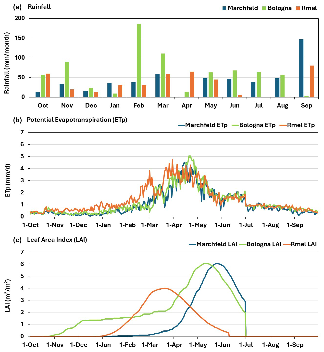
Figure A1 Seasonal patterns (October–September) of key hydroclimatic and vegetation variables at the Marchfeld, Bologna, and Rmel sites. (a) Monthly rainfall distribution. (b) Annual variation in potential evapotranspiration (ET_p). (c) Annual variation in Leaf area index (LAI).

Appendix B: FLOWS model configuration and parameterization

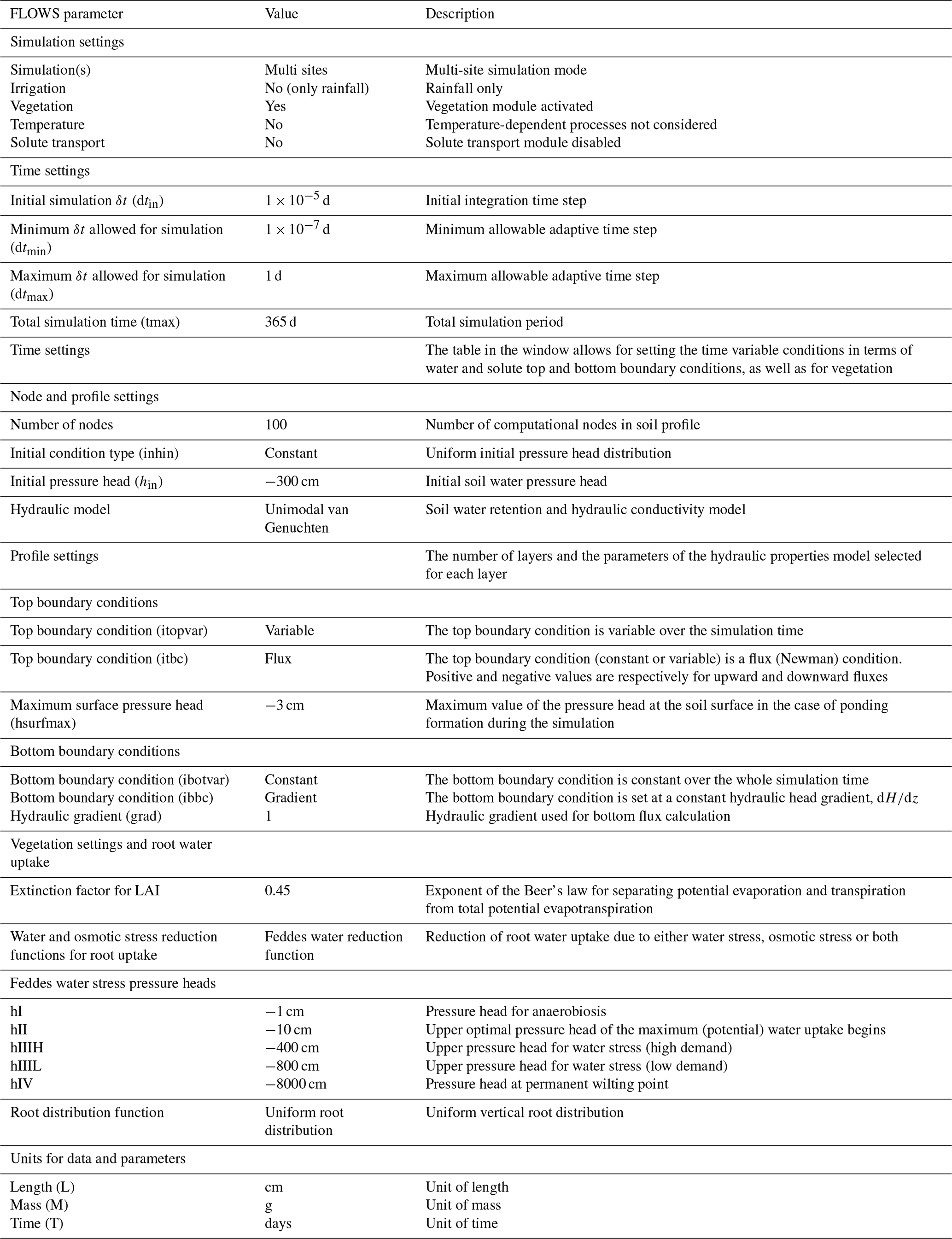
This appendix provides a complete description of all numerical, hydraulic, boundary condition, and vegetation-related parameters used in the FLOWS model within the present study (Table B1).

Table B1 FLOWS model configuration and parameterization used in the simulations, as defined in the FLOWS graphical user interface and handbook (Coppola et al., 2025).