Assessing the potential of complex artificial neural networks for modelling small-scale soil erosion by water

Modelling soil erosion by water is essential for developing effective mitigation strategies and preventing on- and off-site damages in agricultural areas. So far, complex artificial neural networks have rarely been applied in small-scale soil erosion modelling, and their potential still remains unclear. This study compares the performance of different neural network architectures for modelling soil erosion by water at a small spatial scale in agricultural cropland. The analysis was based on erosion rate data (in t ha⁻¹ yr⁻¹) at a 5 m × 5 m resolution, derived from a 20-year monitoring programme, and covers 458 ha of cropland across seven investigation areas in northern Germany. Nineteen predictor variables related to topography, climate, management, and soil properties were selected as inputs to assess their interrelationships with observed erosion patterns. A single-layer neural network (SNN), a deep neural network (DNN), and a convolutional neural network (CNN) were applied and evaluated against a random forest (RF) model used as a benchmark. A leave-one-area-out validation was applied to evaluate how well the models generalize to areas withheld entirely during training. While all models tended to underestimate high erosion rates, they often successfully captured the underlying spatial patterns. All tested models exhibited comparable root mean squared errors (RMSE: 2.2 t ha⁻¹ yr⁻¹). With respect to mean absolute error (MAE), the neural network models achieved slightly lower values (MAE: 0.9 t ha⁻¹ yr⁻¹) than the random forest model (MAE: 1.0 t ha⁻¹ yr⁻¹). Clearer differences between models were observed for the F₁ scores, which reflect performance across soil loss classes. Here, the CNN achieved the highest F₁ score (0.46) among the tested models. This study demonstrates the potential of complex neural networks to capture erosion patterns at the field-to-landscape scale and provides insights into the relevance of the chosen predictor variables, as well as key modelling limitations, such as the underestimation of very high erosion rates in unseen areas. It also highlights the need for more comprehensive datasets to improve generalization capabilities of the models.

1 Introduction

Soil erosion by water causes the loss of topsoil, along with the displacement of organic carbon and nutrients, degrading agricultural land and contributing to off-site damages such as water eutrophication and road blockages (Issaka and Ashraf, 2017). These processes have significant and long-lasting environmental and economic consequences in affected areas worldwide. A combination of anthropogenic, climatic, topographic, and pedological factors unique to each region defines the extent and distribution of soil erosion by water. Modelling the interactions among these factors at fine spatial scales can help reveal key drivers and the resulting erosion patterns. The resulting insights can support the development of targeted strategies to mitigate further soil degradation (Borrelli et al., 2018; Igwe et al., 2017).

Various approaches have been applied to estimate soil erosion by water across different spatial scales, ranging from global (Guerra et al., 2020), continental (Panagos et al., 2021), national (Plambeck, 2020), to small field plots (Anache et al., 2018). The respective modelling approaches vary in data requirements, input variables, underlying principles, and complexity. Model outputs are typically classified into erosion severity, susceptibility categories or expressed as continuous predictions of soil erosion rates over space and time. Depending on the intended output and available data, a variety of model types have been developed, including process-based, empirical, and, more recently, machine learning models (Borrelli et al., 2021).

Examples of physical process-based models are WEPP (Nearing et al., 1989; Pieri et al., 2007), Erosion 3D (Schmidt et al., 1999), and EUROSEM (Morgan et al., 1998). Empirical models include the Universal Soil Loss Equation (USLE; Wischmeier and Smith, 1978), its revised version (RUSLE; Renard et al., 1997), and further adaptations (Borrelli et al., 2021). One reason for the popularity of the USLE and its variations is their relatively low complexity, making these models time- and cost-efficient (Alewell et al., 2019; Avand et al., 2023; Kumar et al., 2022). The apparent simplicity of the USLE contrasts with the complexity of calculating its individual factors, which results in a wide range of individual USLE-based applications and estimated loss rates due to variations in input data and methods (Fiener et al., 2020).

Machine learning approaches have been increasingly used to identify areas at risk of soil erosion by water and to capture the complex relationships between environmental predictors and observed erosion patterns. This includes the application of methods such as random forests (RF; Garosi et al., 2019; Ghosh and Maiti, 2021; Jaafari et al., 2022), with several studies reporting that RF can outperform methods such as support vector machines (SVMs) and generalized additive models (GAMs). While these studies highlight the potential of RF models, their main focus has been on predicting and classifying gully-erosion susceptibility.

Another promising machine learning approach for soil erosion modelling is the application of artificial neural networks (ANNs). However, existing studies in this field have often employed simple neural network architectures, typically with only a single hidden layer. These single-layer networks have not only been used to model soil erosion susceptibility (De la Rosa et al., 1999) but also to predict quantitative soil erosion rates at the plot scale (Licznar and Nearing, 2003). These early applications demonstrate the potential of ANNs, but single-layer networks may not fully utilize the capacity of more complex architectures to capture non-linear relationships between influencing variables and the spatial distribution and magnitude of soil erosion (Avand et al., 2023).

More complex, multi-layered ANNs have rarely been applied to predict soil erosion rates quantitatively. Instead, they have been mostly used to model a classified erosion susceptibility (Golkarian et al., 2023; Khosravi et al., 2023; Sarkar and Mishra, 2018) or have been restricted to gully erosion (Ghorbanzadeh et al., 2020; Saha et al., 2021). In cases where ANNs have been applied to quantify continuous soil erosion rates, studies often rely on limited datasets, such as those collected using erosion pins over just one year (Gholami et al., 2021; Sahour et al., 2021).

While machine learning methods have shown promise in modelling soil erosion, their application to predict continuous erosion rates at fine spatial scales remains limited, particularly when using neural networks. Currently, most studies rely on input data with spatial resolutions between 5 and 300 m, with higher-resolution datasets often restricted to small areas, such as individual plots (Borrelli et al., 2021; Parsons, 2019). This lack of research combining neural networks with high-resolution data is partly due to the limited availability of long-term monitoring schemes at the landscape scale, which provides spatially explicit erosion data as ground truth for model training and validation (Batista et al., 2025).

To address this gap, this study utilized long-term soil erosion monitoring data spanning more than two decades and collected across seven study areas in northern Germany (Steinhoff-Knopp and Burkhard, 2018). This monitoring dataset, together with high-spatial-resolution predictor variables, served as input for different machine learning models. Specifically, three neural networks of increasing complexity and a random forest, used as a benchmark model, were systematically compared to evaluate their ability to predict continuous soil erosion rates. To assess model robustness and generalizability, we applied a leave-one-area-out validation strategy, in which each study area was withheld in turn for testing while the models were trained on the remaining areas.

The goal of this study was to contribute to a more comprehensive understanding of the strengths and limitations of different machine learning approaches for soil erosion modelling by aiming to answer the following research questions:

1. Which machine learning approach achieves the highest predictive performance in estimating spatial patterns of continuous soil erosion rates at the field-to-landscape scale?

2. What are the challenges and limitations when reproducing erosion patterns within the same areas and when extrapolating to previously unseen areas?

3. Which predictor variables are most important for predicting soil erosion by water at the field-to-landscape scale across different machine learning models?

2 Methods

2.1 Study area

This study uses data from seven distinct study areas in Lower Saxony, Germany, located between 53.1 and 51.9°N latitude and 8.3 and 10.5° E longitude. Five of these regions are clustered in the southeastern part of Lower Saxony, and named Leine-Innerstebergland, while the other two are located in the Northeast and Southwest (Fig. 1). The cultivated cropland within all the areas covers 458 ha, is prone to erosion, and represents different soil types, relief characteristics, and management conditions (Capelle and Lüders, 1985; Capelle, 1990).

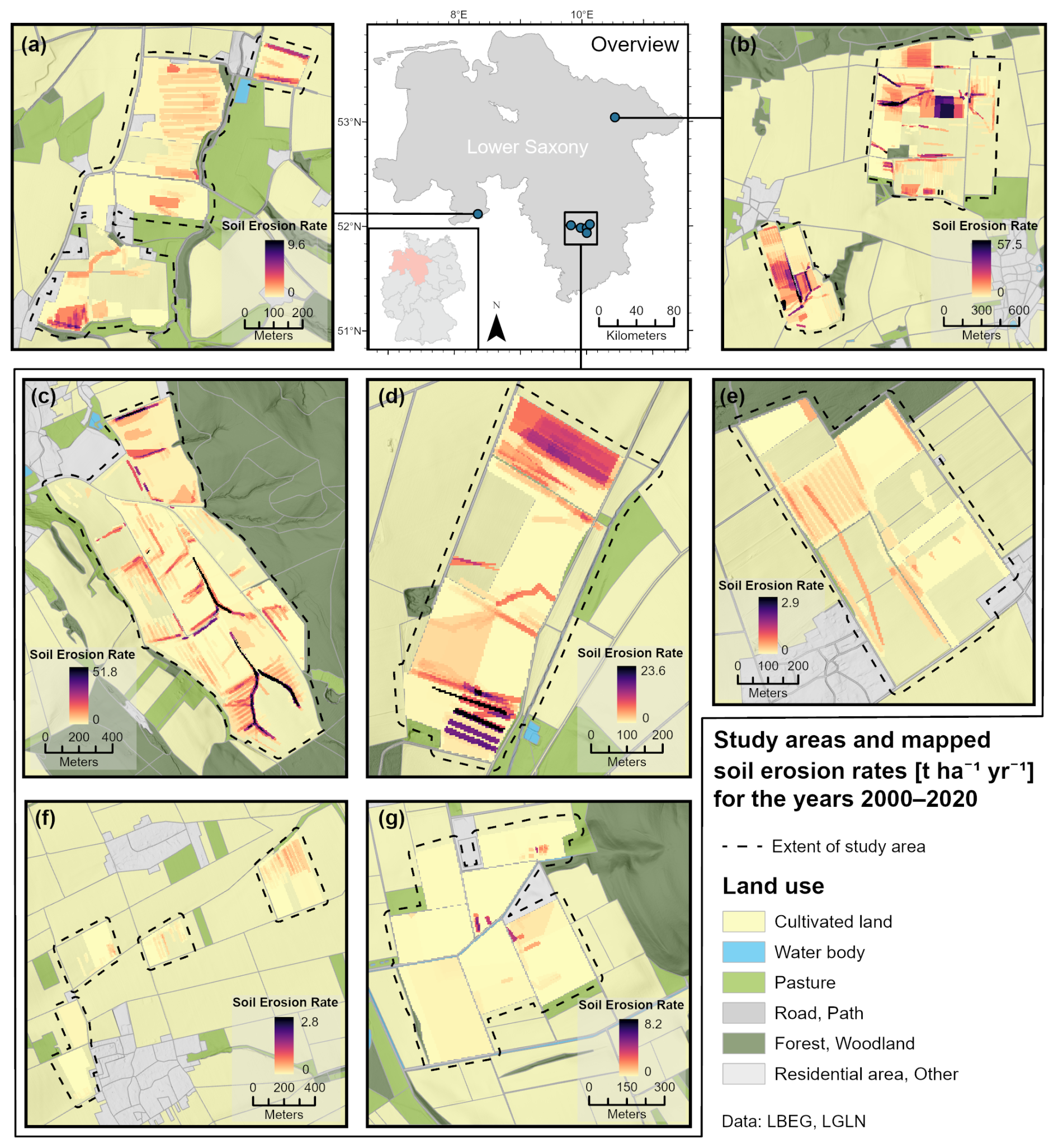
Figure 1 Overview of study areas in Lower Saxony and mapped soil erosion rates in (a) Küingdorf, (b) Barum, (c) Lamspringe, (d) Klein Ilde, (e) Nette, (f) Adenstedt, and (g) Brüggen.

A large part of the soils – predominantly Luvisols and Cambisols – has a high silt content due to loess or sand-loess deposits, which results in higher topsoil erodibility (Steinhoff-Knopp and Burkhard, 2018). The mean slope across all study areas is 4.01°, with the southern regions having a steeper relief (4.81°) compared to the northern (2.35°) and the western region (3.68°). The primary crops by cultivated area are winter wheat, followed by winter barley, rapeseed, sugar beet, maize, and potatoes. All farmers within the monitored areas practice conventional farming and implement various soil conservation practices, including reduced tillage, contour-parallel tillage, cover crops, grassed tramlines, and drainage systems.

2.2 Data collection

The soil erosion dataset used in this study was derived from a long-term monitoring programme funded by the Lower Saxony State Authority for Mining, Energy and Geology (LBEG), covering the years 2000 to 2020. Exceptions are the investigation areas Adenstedt, where monitoring began in 2002, and Klein Ilde, where monitoring stopped in 2015. The methodology of the field surveys is based on the recommendations by Rohr et al. (1990) and the instructions by DVWK (1996) and Botschek et al. (2021). To implement a more efficient workflow, the mobile mapping application EroPad was used since 2010 (see Steinhoff et al., 2013). The field surveys were carried out each year after the snowmelt (usually in February or March) throughout the vegetation period and typically within one week after each erosive rainfall event (≥10 mm total rainfall or >10 mm h⁻¹ within 30 min), following the German definition of erosive rainfall events in place during the monitoring period (see DIN, 2005, 2017; Schwertmann et al., 1987). Mapping in early spring (after the snowmelt) records cumulative erosion caused by snowmelt and single precipitation events during the winter agricultural dormant period. Surveys were also conducted when farmers reported erosion features.

The field surveys aimed to collect data on the spatial distribution and extent of three main types of soil erosion by water: linear (i.e. rill) erosion, sheet erosion, and sheet-to-linear erosion (erosion systems showing both features of sheet and linear erosion). The losses by linear erosion features were surveyed by measuring their volume and extrapolated to an 8 m buffer around their occurrence to account for the dispersion of soil loss due to tillage practices by farmers. Deposition sites were also recorded, but only qualitatively, and were therefore not included in the modelling. A detailed description and evaluation of the survey dataset is provided in Steinhoff-Knopp and Burkhard (2018). For the modelling process, soil erosion rates (t ha⁻¹ yr⁻¹) were calculated by overlaying all surveyed erosion features in a grid resolution of 5 m × 5 m (Fig. 1).

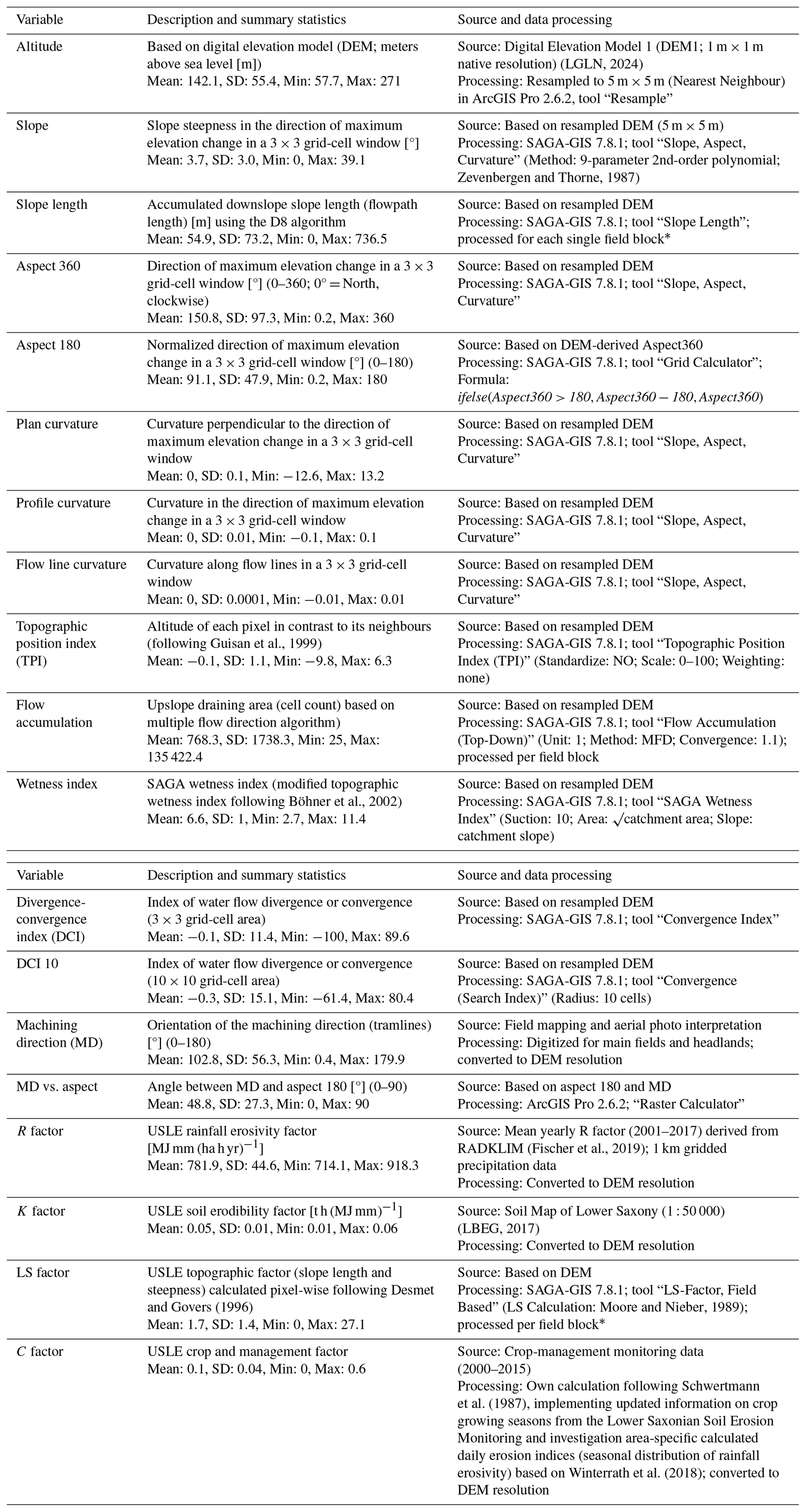
Table 1 Overview of the variables used in the soil erosion modelling process. A detailed description, including processing steps, can be found in Appendix A1.

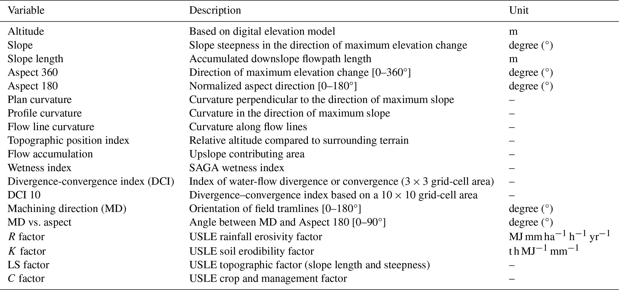
Nineteen predictor variables (i.e. features or covariates) potentially influencing soil erosion were selected for the modelling process (Table 1). Further information on the methods to determine each predictor variable is provided in Appendix A1. The variables include factors related to topography, climate, soil properties, and agricultural land management. The topographic variables were derived from a digital elevation model (DEM) with a native resolution of 1 m × 1 m, resampled to 5 m × 5 m, which serves as the basis for all derived topographic variables. The USLE R factor (erosivity of rainfall), originally calculated at a grid resolution of 1 km × 1 km, was aligned with the DEM-based variables by directly assigning the values of the corresponding 1 km pixels without further modification. The USLE K factor (erodibility of topsoil), derived from a soil map at a scale of 1 : 50 000 (LBEG, 2017), and the USLE C factor (crop cover and management factor) were rasterized to the 5 m × 5 m grid. The C factor was determined for each field using agricultural land management data collected during the field surveys and through interviews with the respective farmers.

Several of the variables, especially the topographic variables, were derived from each other or capture related aspects, which could lead to a strong correlation between them (Avand et al., 2023; Jaafari et al., 2022). Therefore, the degree of the linear relationship between variables was assessed by using the Pearson correlation coefficient and the variance inflation factor (VIF). The Pearson correlation coefficient is used to gain information on the pairwise linear correlation between the variables, with ±0.7 being considered a threshold for strong correlation (Schober et al., 2018). The VIF is used to assess multicollinearity across all variables, evaluating whether variables with high pairwise correlations can still provide valuable information for the final predictions (Ebrahimi-Khusfi et al., 2021; O'Brien, 2007). Variables with a VIF below 5 are considered to have a low level of multicollinearity and are used for the modelling (Daoud, 2017).

2.3 Machine learning models

This section provides a brief introduction to the four distinct machine learning models employed in this study. The model implementations and hyperparameter selection process are described in Sect. 2.5.

2.3.1 Random forest

A random forest (RF) model combines multiple decision trees to create an ensemble model to improve prediction accuracy (Breiman, 2001). A decision tree splits data based on feature values across multiple levels of nodes, with each branch representing different decision paths leading to predictions (Kingsford and Salzberg, 2008). Each tree is trained on a random subset of the variables, and, in the case of regression tasks, as applied in this study, the final prediction is obtained by averaging the outputs of all trees.

Although mostly limited to classification outputs, RF has shown promise in previous studies on soil erosion modelling (Garosi et al., 2019; Ghosh and Maiti, 2021; Jaafari et al., 2022). Therefore, in this study, RF serves as a benchmark for evaluating the performance of neural networks against other machine learning models. The RF model used in this study consisted of 400 decision trees, with a maximum tree depth of 20, a minimum of two samples required to split an internal node, and at least one sample per leaf.

2.3.2 Single-hidden layer neural network

Artificial neural networks consist of an input layer, an output layer, and one or more so-called hidden layers of neurons (or nodes) in between (Rumelhart et al., 1986). Each neuron in these layers is interconnected through weights. During training, these weights are updated through an optimization process involving multiple iterations, a loss function, and, most commonly, backpropagation. The weighted sum of the inputs is passed through an activation function, which applies a non-linear transformation to determine the neuron's output, which is then passed on to the subsequent layer. In a fully connected (or dense) layer, each neuron is connected to every neuron in the subsequent layer through individual weights.

Three different types of neural networks were compared in this study, each with a distinct and increasingly complex architecture. The first type is a neural network with a single dense layer (SNN) of 512 neurons between the input and the output layer (see Wythoff, 1993). The Rectified Linear Unit (ReLU) activation function was applied in both the hidden and output layers in this and the following two variations of neural network models, to introduce non-linear relationships and constrain predictions to positive values (see Krizhevsky et al., 2017; Nair and Hinton, 2010). Additionally, L₂ regularization, also known as Ridge regularization, was employed across all neural networks to reduce overfitting (see Hoerl and Kennard, 1970; Ng, 2004). The Adam optimizer was used to determine the learning rate during training (see Kingma and Ba, 2014).

2.3.3 Deep neural network

The interconnected neurons and the corresponding weights enable neural networks to capture complex non-linear relationships. Increasing the number of hidden layers enhances this capability while increasing training time and the likelihood of overfitting the model to the training data. Such a neural network with multiple hidden layers is commonly known as a deep neural network (DNN) or a deep learning model (LeCun et al., 2015). In this case, the DNN was modified to have three hidden layers, each with 256 neurons.

2.3.4 Convolutional neural network

Convolutional neural networks (CNNs) are specifically designed to capture spatial relationships in grid-like data structures, such as images (LeCun et al., 2015). This is achieved through convolutional layers that receive input patches containing the neighbouring grid cells around each target pixel. These patches provide local spatial context, enabling the network to learn spatial patterns and relationships relevant for predicting soil erosion (Krizhevsky et al., 2017; LeCun et al., 2015). In this study, each input consisted of a 7 × 7 grid-cell patch. Within these patches, the convolutional layers extracted spatial features using 256 filters per layer. Two dense layers with 256 neurons each were added following the four convolutional layers. The dense layers utilize the learned spatial patterns from the convolutional layers to produce the final predicted output.

2.4 Validation metrics

The results were compared using different validation metrics. To determine the overall differences between the modelled and the mapped soil erosion rate, the root mean squared error (RMSE) and the mean absolute error (MAE) were used. As soil erosion is commonly reported in severity classes (e.g. Borrelli et al., 2018; Steinhoff-Knopp and Burkhard, 2018), we additionally evaluated classification performance using the F₁ score (harmonic mean of precision and recall) to assess the ability of the models to predict different ranges of soil erosion severity (Chinchor, 1992). For this, the continuous predicted output was categorized into six discrete classes: no erosion (0 t ha⁻¹ yr⁻¹), very low erosion (>0 to <0.25 t ha⁻¹ yr⁻¹), low erosion (0.25 to <1 t ha⁻¹ yr⁻¹), medium erosion (1 to <2 t ha⁻¹ yr⁻¹), high erosion (2 to <5 t ha⁻¹ yr⁻¹), and very high erosion (≥5 t ha⁻¹ yr⁻¹). A weighted average F₁ score was calculated to account for the imbalanced distribution of the mapped soil erosion dataset across the classes, with the majority (81.2 %) of the data falling below 1 t ha⁻¹ yr⁻¹. The resulting F₁ score ranges from 0 to 1, with values closer to 1 indicating a better overall alignment between the prediction and the different classes (Taha and Hanbury, 2015).

The importance of the predictor variables was evaluated through permutation importance, which reflects the influence of each variable on the final model output. This is done by randomly permuting one variable at a time and measuring the resulting increase in the mean squared error. A larger increase indicates that the variable has a greater impact on the predictive performance of the model. The results are normalized and expressed as percentages (Altmann et al., 2010).

2.5 Model implementation

To evaluate model predictions, we employed a leave-one-area-out validation strategy, in which one study area was excluded entirely during model training and subsequently used for validation. In each iteration, the models were trained on the remaining six areas and then used to predict soil erosion rates in the left-out area. Afterwards, the predictions were validated against the mapped erosion rates of that area. This procedure was repeated for all seven study areas, and validation metrics were calculated as weighted averages based on the relative size of the excluded area. Permutation importance values were also averaged across all seven runs. Using this validation approach enabled a comprehensive assessment of model robustness by evaluating their capacity to generalize to unseen areas with varying landscape conditions and management practices.

The predictive performance of each model depends strongly on its hyperparameters, which determine the model architecture and learning behaviour. The most important hyperparameters (e.g. number of trees or neurons) and their optimal values were described along with the respective models above (Sect. 2.3). To determine the optimal hyperparameters without any data leakage, a nested cross-validation procedure was implemented, where the left-out area was reserved exclusively for final evaluation. Hyperparameter tuning was performed on the remaining six areas using an inner leave-one-area-out procedure. This process was repeated for each study area. The final hyperparameter configuration was determined from the aggregated inner validation performance and subsequently used to retrain the model on the six training areas before evaluation on the left-out test area. To limit computational demand, hyperparameters were optimized using a random search strategy (Bergstra and Bengio, 2012; Yu and Zhu, 2020). The full search space and tuning scripts are provided in the accompanying repository.

All predictor variables were standardized and the soil loss target was log-transformed to reduce skewness and stabilize model training. Predicted values were back-transformed to the original scale for evaluation and visualization. All models were built using the scikit-learn (Pedregosa et al., 2011) and TensorFlow (Abadi et al., 2015) Python packages.

3 Results

3.1 Pairwise correlation and multicollinearity analysis

To assess relationships between predictor variables and to identify potential redundancy due to multicollinearity, the Pearson correlation coefficient (r) and the variance inflation factor (VIF) were calculated. Five pairs of variables (see Fig. B1 in Appendix B) had a strong linear correlation with Pearson coefficient close to or exceeding ±0.7: aspect 360 and slope length (r=0.69), slope and machining direction ($r=-\mathrm{0.69}$), altitude and R factor ($r=-\mathrm{0.75}$), topographic position index and divergence-convergence index 10 (r=0.82), divergence-convergence index and wetness index (r=0.82). However, all variables had a VIF < 5, indicating that there is not a high level of multicollinearity between the variables (see Fig. B2). Consequently, no variables were removed for the modelling process.

3.2 Model performance

Overall, the neural networks produced nearly identical error metrics when predicting soil erosion rates in previously unseen areas (Table 2). All models achieved an RMSE value of 2.2 t ha⁻¹ yr⁻¹, with corresponding 95 % confidence intervals (CI) across areas ranging from 1.2–2.6 for RF and DNN and 1.3–2.6 for SNN and CNN. The MAE ranged from 0.9 t ha⁻¹ yr⁻¹ for the neural networks to 1.0 t ha⁻¹ yr⁻¹ for the RF, with overlapping 95 % confidence intervals showing no meaningful differences among models in this regard (RF: 0.7–1.2; SNN and DNN: 0.6–1.1; CNN: 0.6–1.2).

Table 2 RMSE and MAE (in t ha⁻¹ yr⁻¹) differentiated by soil erosion rate class for the random forest (RF), single-layer neural network (SNN), deep neural network (DNN), and convolutional neural network (CNN) models.

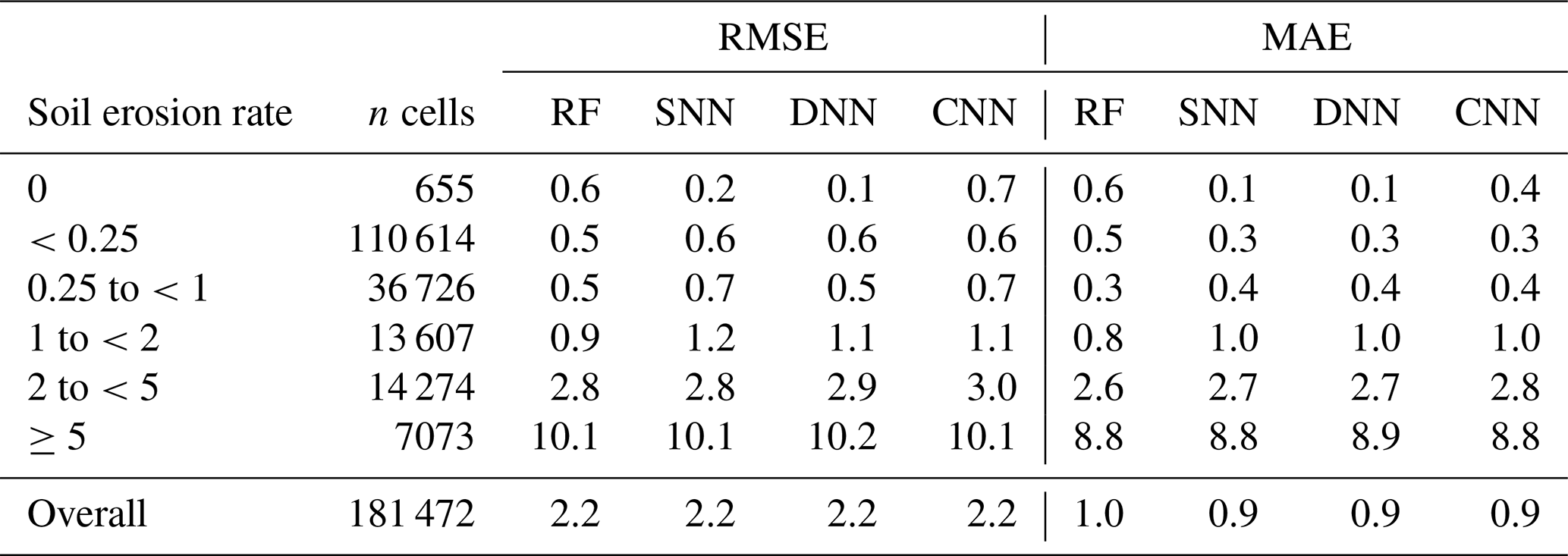
Table 3 F₁ score evaluating the performance of the continuous model predictions (in t ha⁻¹ yr⁻¹) within the defined soil erosion rate classes, comparing random forest (RF), single-layer neural network (SNN), deep neural network (DNN), and convolutional neural network (CNN) models. The weighted average F₁ scores were computed using the number of mapped grid cells (n cells) within each class.

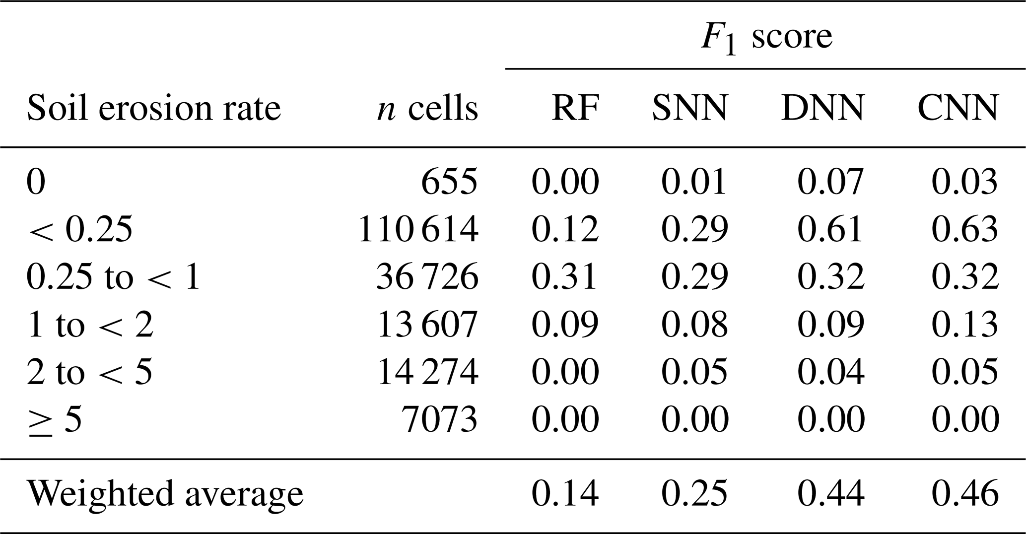
The F₁ scores shown in Table 3 illustrate some differences in model performance for low soil erosion rates by measuring how well the continuous predictions align within the defined severity classes. Although F₁ scores were generally low, the CNN achieved the highest weighted average value (0.46; 95 % CI: 0.39–0.55), followed closely by the DNN (0.44; 95 % CI: 0.38–0.55)), whereas the RF and SNN performed substantially worse in this regard, with an F₁ score of 0.14 (95 % CI: 0.09–0.17) and 0.25 (95 % CI: 0.19–0.27), respectively. The differences are largely linked to the <0.25 t ha⁻¹ yr⁻¹ class, which contained the majority of mapped grid cells. Here, the CNN and DNN achieved high F₁ scores of 0.63 and 0.61, compared with 0.12 for the RF and 0.29 for the SNN. For erosion rates equal and above 5 t ha⁻¹ yr⁻¹, all models had an F₁ score of 0.

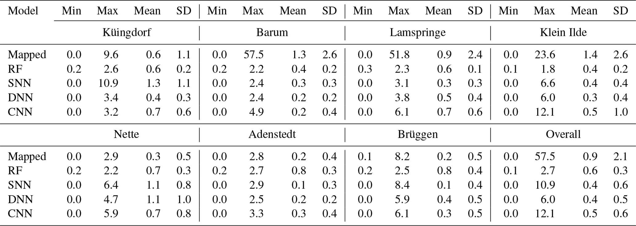
Across all study areas, the maximum predicted soil erosion rates ranged from 2.7 t ha⁻¹ yr⁻¹ predicted by the RF to 12.1 t ha⁻¹ yr⁻¹ predicted by the CNN (Table C1 in Appendix C). The soil erosion predictions of the DNN are shown in Fig. 2. The corresponding prediction maps for all models are provided in Appendix C (Figs. C1–C8). The predictions show that all models were partially able to predict the spatial distribution of erosion features in the unseen areas. In several areas, such as Küingdorf, Lamspringe, and Adenstedt (Fig. 2a, c, f), the prediction shows spatial patterns comparable to those in the mapped data. However, the models did not consistently reproduce erosion structures in the other areas, and the severity of some high-erosion features was underestimated (e.g. Barum, Fig. 2b).

Figure 2 Predicted soil erosion rates using the leave-one-area-out approach by the deep neural network (DNN) in (a) Küingdorf, (b) Barum, (c) Lamspringe, (d) Klein Ilde, (e) Nette, (f) Adenstedt, and (g) Brüggen.

The difference between the predicted soil erosion rate by the DNN and mapped erosion rates is shown in Fig. 3. The visualization shows that the few high erosion features within the study areas of Barum, Lamspringe, and Klein Ilde (Fig. 2b, c, d) are strongly underestimated. In contrast, in the study areas of Küingdorf, Nette, Adenstedt, and Brüggen (Fig. 2a, e, f, g), the difference between modelled and mapped soil erosion was mostly below 5 t ha⁻¹ yr⁻¹, with no large over- and underestimations. Locations with low mapped erosion rates (<1 t ha⁻¹ yr⁻¹) were generally predicted within the same order of magnitude as the mapped values, which is supported by the F₁ scores (Table 3).

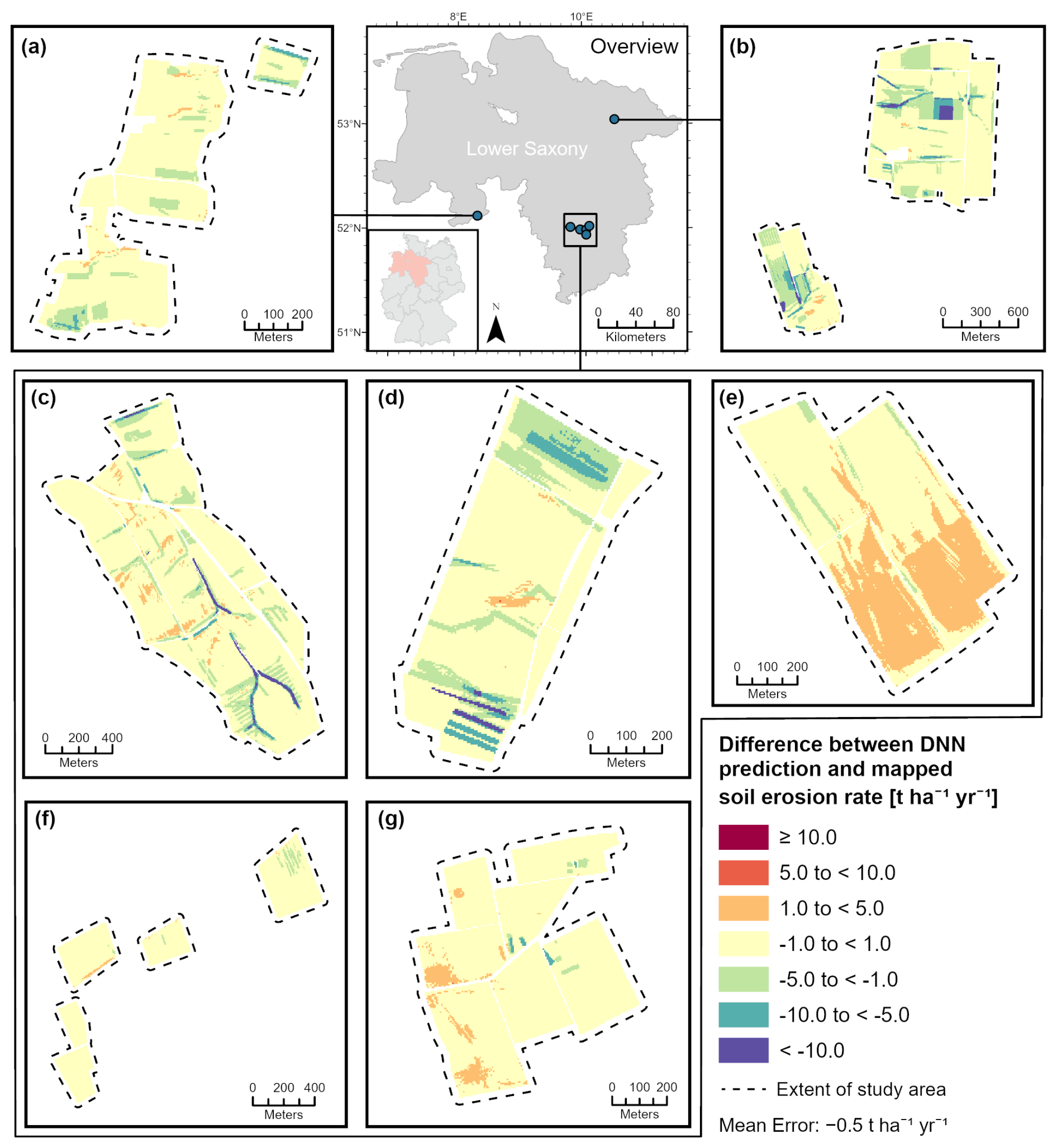
Figure 3 Difference between soil erosion rates predicted by the deep neural network (DNN) and the mapped values in (a) Küingdorf, (b) Barum, (c) Lamspringe, (d) Klein Ilde, (e) Nette, (f) Adenstedt, and (g) Brüggen, where positive values indicate overestimation of the model and negative values indicate underestimation.

3.3 Variable importance

The permutation importance results are shown in Fig. 4. While slope showed consistently high importance across all models, with an average contribution of 18.6 %, the ranking of several other predictors varied noticeably between models. For instance, the CNN assigned comparatively high importance to the Wetness index (20.2 %) and the RF attributed its highest importance to the LS factor (18.2 %). The SNN and DNN relied strongly on slope (≥26.5 %). Machining direction vs. aspect was the second most important variable for RF, SNN and DNN.

Several variables exhibit consistently low importance (<5 %) across all models, including aspect (360 and 180), the divergence–convergence index, flowline curvature, plan curvature, and profile curvature. These predictors contributed to a small extent, if at all, to the model performance.

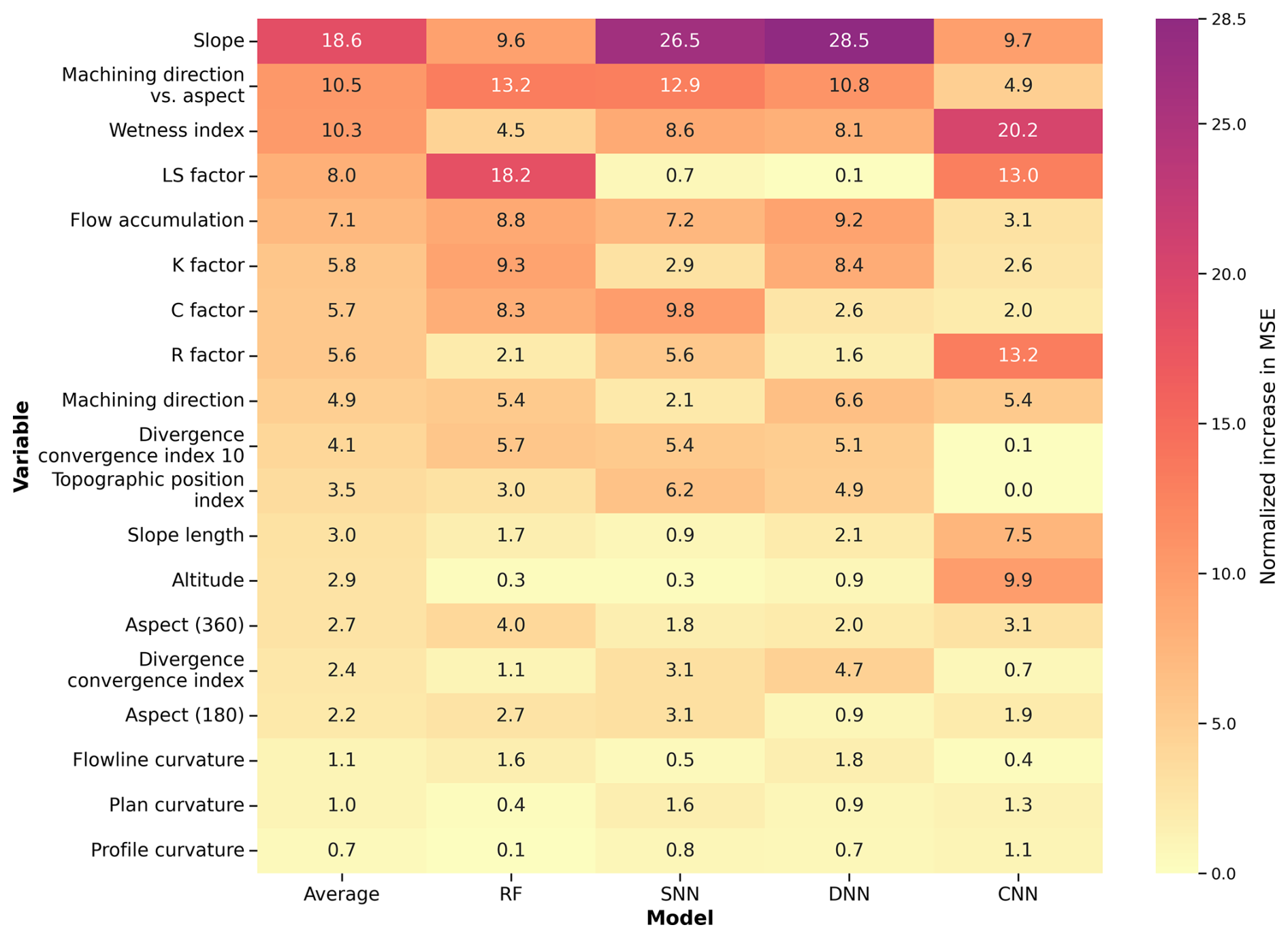
Figure 4 Heatmap of the permutation importance of all predictor variables, shown for the overall average across models and for the random forest (RF), single-layer neural network (SNN), deep neural network (DNN), and convolutional neural network (CNN). Values represent the normalized increase in mean squared error (MSE) after permuting each variable.

4 Discussion

4.1 Comparison of model performance

Large neural networks have the capacity to capture complex non-linear relationships between predictor variables and soil erosion rates through an extensive set of weights. This flexibility allows neural networks to model these relationships in greater detail. In our study, the neural network models showed comparable or slightly improved predictive performance relative to the RF. However, in terms of class-based validation metrics (Table 3), the CNN and DNN outperformed the RF and SNN predictions. In this regard, the results align with previous studies, such as Sarkar and Mishra (2018), indicating that increasing model complexity can improve predictive performance.

A large proportion (81.2 %) of the mapped data is below the threshold of 1 t ha⁻¹ yr⁻¹, and this value range therefore had a strong influence on the weighted average F₁ score. As a result of underestimating these low erosion rates, the RF achieved a lower weighted average F₁ score than the neural network based models. The neural networks, and particularly the CNN and DNN, were able to predict these low erosion rates moderately well, capturing the underlying relationships in this dominant class.

This strong class imbalance and the dominance of low soil erosion values within the dataset also affect the capability of the models to predict higher erosion rates. Additionally, while the applied log-transformation stabilises model training, it further reduces the influence of extreme erosion values. As shown in Table 3, all models fail to reproduce very high erosion rates (≥5 t ha⁻¹ yr⁻¹). Since these high values are rare, representing only 3.9 % of the overall mapped training data, they provide too few examples for the models to learn the corresponding relationships reliably, which is a common problem in soil science for prediction tasks using machine learning (Sharififar and Sarmadian, 2023). In addition, the left-out areas have different landscape structures, land management practices, and topographic patterns, leading to combinations of predictor variables that the models have not encountered during training. This distribution shift places many erosion features outside the range of conditions represented during training, making accurate prediction in previously unseen areas particularly challenging. For example, the underestimation in Barum can be explained by substantial differences in crop rotations compared to other monitoring areas, resulting in a higher C factor that was not represented in the respective training data.

As shown in the visualizations of the predictions (e.g. Figs. 2 and 3), all models were able to reproduce parts of the spatial erosion patterns in the unseen areas, although the predicted magnitudes were often underestimated. Only the neural network models predicted very high soil erosion rates, with maximum values of 6.0 and 12.1 t ha⁻¹ yr⁻¹, respectively. Both SNN and DNN produced very similar soil erosion patterns, likely due to the comparable architectures of the two modelling approaches, despite differences in their complexity. The CNN output appeared notably smoother than that of the solely pixel-based models, albeit with a lower maximum predicted erosion rate. This smoothness can be attributed to the integration of local spatial context by the convolutional layers (Fu et al., 2019; Hilburn, 2023).

While the RF, SNN, and DNN train on a pixel by pixel basis, the CNN potentially benefits from incorporating local spatial context through input patches that include neighbouring grid cells during training. However, the results show only very small differences between the evaluation metrics of all models. Although the CNN and DNN achieved the highest F₁ scores, all models exhibited nearly identical overall RMSE and MAE.

It is also important to note that the DNN, and particularly the SNN and RF models, require significantly fewer computational resources than the CNN, which can be beneficial when trained on big datasets or when the model is applied to predict soil erosion for larger areas. Therefore, depending on the specific use case, the potential trade-off between potentially improved predictive performance and the increased complexity and computational demands of large neural networks, such as the CNN should be carefully considered.

The permutation-importance analysis highlights the combined influence of topographic and anthropogenic (i.e. land management) variables on soil erosion. For example, the high importance of the predictor variable machining direction vs. aspect is likely explained by the large proportion of mapped erosion features occurring in tramlines aligned with the slope direction (Steinhoff-Knopp and Burkhard, 2018). The permutation analysis also reveals clear differences between the modelling approaches. These differences can be attributed to the respective model architectures. The RF relied on a hierarchical split structure, which caused it to prioritize variables that repeatedly improve node splits across trees, resulting in an importance pattern that differs from that of the neural networks (Breiman, 2001). The SNN and DNN relied strongly on similar predictor variables (e.g. slope and machining direction vs. aspect), indicating that their similar architectures resulted in comparable learned non-linear relationships between predictors and soil erosion (LeCun et al., 2015; Nielsen, 2015). The CNN, by applying convolutional filters over spatial neighbourhoods, prioritizes variables that contribute to local spatial patterns rather than relying solely on single-pixel attributes (LeCun et al., 2015). Consequently, the models emphasize different predictors when optimizing performance in previously unseen areas. Despite these architectural differences, a consistent result across all models is that aspect, the divergence–convergence index, flowline curvature, plan curvature, and profile curvature show very low importance and contribute little to predicting soil erosion in this study.

4.2 Limitations and future research

Typical challenges and limitations in soil erosion modelling at the landscape scale include the high range of input variables from different domains for parametrization, leading to simplification in variable estimation and mismatches in the scale of input and output data, the application of models outside of the validation range, and inherent restrictions of the used models. This study addressed several of these limitations by utilizing a dataset based on a long-term soil erosion monitoring programme across multiple study areas, capturing long-term patterns of soil erosion by water within these regions. Additionally, input variables with relatively high spatial resolution were incorporated into machine learning models capable of capturing non-linear relationships at varying levels of complexity. Despite these approaches, several challenges and limitations remain. These challenges and limitations should be considered when interpreting the results and highlight key areas for future research to enhance small-scale soil erosion predictions.

The results demonstrate that complex neural networks can partially reproduce erosion patterns when extrapolating to previously unseen areas. However, all models exhibited a strong tendency to underestimate soil erosion. This was mainly caused by the strong imbalance in the dataset, which provided too few examples for the models to learn robust relationships for high erosion rates. These findings suggest that a larger representation of high-erosion events within the same landscape may improve the learning capabilities of such extremes. However, whether this would improve spatial pattern prediction requires further testing.

The results indicate that prediction performance shows only a very slight increase with model complexity (Tables 2 and 3), and the differences between the models were small. In particular, differences were observed only for the F₁ score, where CNN and DNN achieved higher values. Whether this generally justifies the use of a more complex architecture, such as a CNN or DNN in soil erosion modelling, must be carefully evaluated based on the aim and context of the respective study. Future research could investigate this further by comparing a broader range of machine learning approaches, such as gradient boosting machines, or by evaluating ensemble methods. In addition, more recent neural network architectures such as transformers (e.g. Liu et al., 2024) may offer more effective prediction capabilities.

This study provides a useful overview of the importance of various variables in modelling soil erosion by water. Since the primary aim was to compare machine-learning approaches rather than to establish a comprehensive predictor set, some factors affecting soil erosion may not have been included or may influence soil erosion by water at spatial scales not fully represented by the selected variables. As a result, the predictions may not fully capture all relevant processes, and further research is needed to assess the impact of additional variables on soil erosion modelling. On the other hand, this study gives applicable guidance on which predictors might be omitted in soil erosion by water modelling.

5 Conclusions

By comparing different artificial neural network architectures and using a random forest model as a benchmark, this study highlights the potential of neural networks for modelling non-linear relationships between predictor variables and soil erosion at a field-to-landscape scale. Overall, all models showed very similar RMSE and MAE values, indicating comparable performance in predicting continuous soil erosion rates. The convolutional neural network achieved a marginally higher F₁ score, followed closely by the deep neural network. When applied to previously unseen areas, all models were able to partially reproduce spatial erosion patterns but tended to strongly underestimate features with high erosion rates. The permutation importance analysis further indicates the relevance of variables such as slope and machining direction vs. aspect. Furthermore, the analysis provides guidance on which predictors may be omitted in soil erosion modelling. To build upon these findings, future research should focus on further identifying and quantifying model uncertainties, as well as improving the generalizability of these models and their scalability to larger areas.

Appendix A: Data collection

(LGLN, 2024)Zevenbergen and Thorne, 1987Guisan et al., 1999Böhner et al., 2002(Fischer et al., 2019)(LBEG, 2017)Desmet and Govers (1996)Moore and Nieber, 1989Schwertmann et al. (1987)Winterrath et al. (2018)

Table A1 Overview of terrain and USLE-related variables, including data sources, processing steps, and summary statistics. Grid cell size of all variables: 5 × 5 m. See column source and data processing for applied resampling methods.

^* Field block: A contiguous agricultural reference parcel bounded by stable landscape features (roads, paths, hedges, ditches, rivers, forests, etc.).

Appendix B: Pairwise correlation and multicollinearity analysis

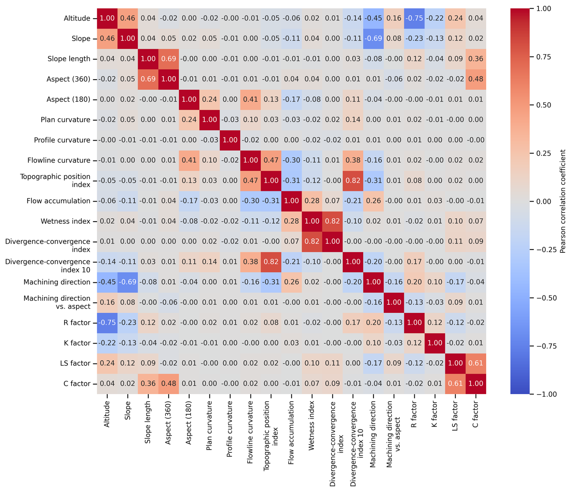
Figure B1 Pairwise linear correlation analysis of all predictor variables used in this study based on the Pearson correlation coefficient.

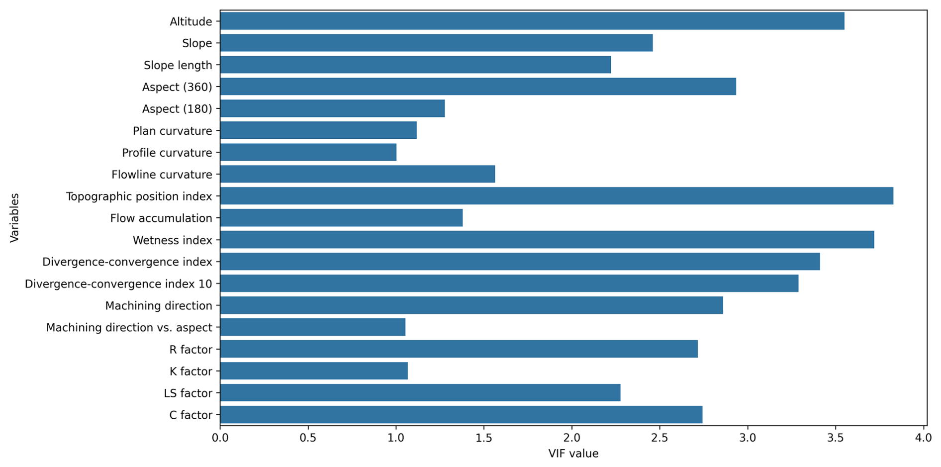
Figure B2 Variance inflation analysis of predictor variables highlights the level of multicollinearity, with higher VIF values indicating greater multicollinearity among predictors.

Appendix C: Results

C1 Raw model predictions

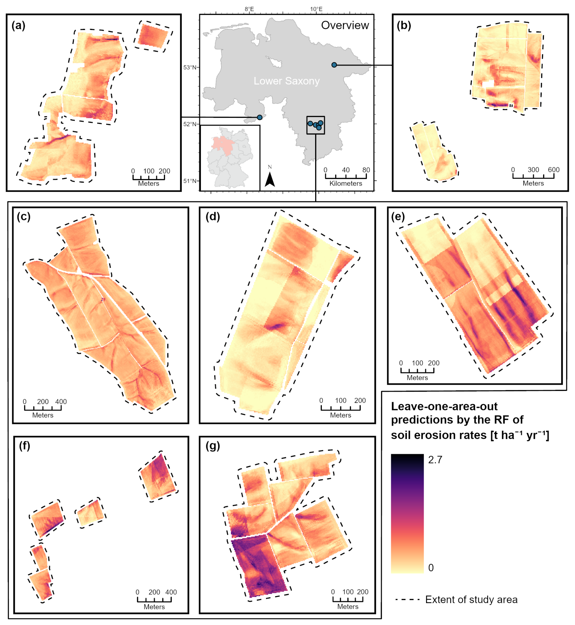
Figure C1 Predicted soil erosion rates using the leave-one-area-out approach by the random Forest (RF) in (a) Küingdorf, (b) Barum, (c) Lamspringe, (d) Klein Ilde, (e) Nette, (f) Adenstedt and (g) Brüggen.

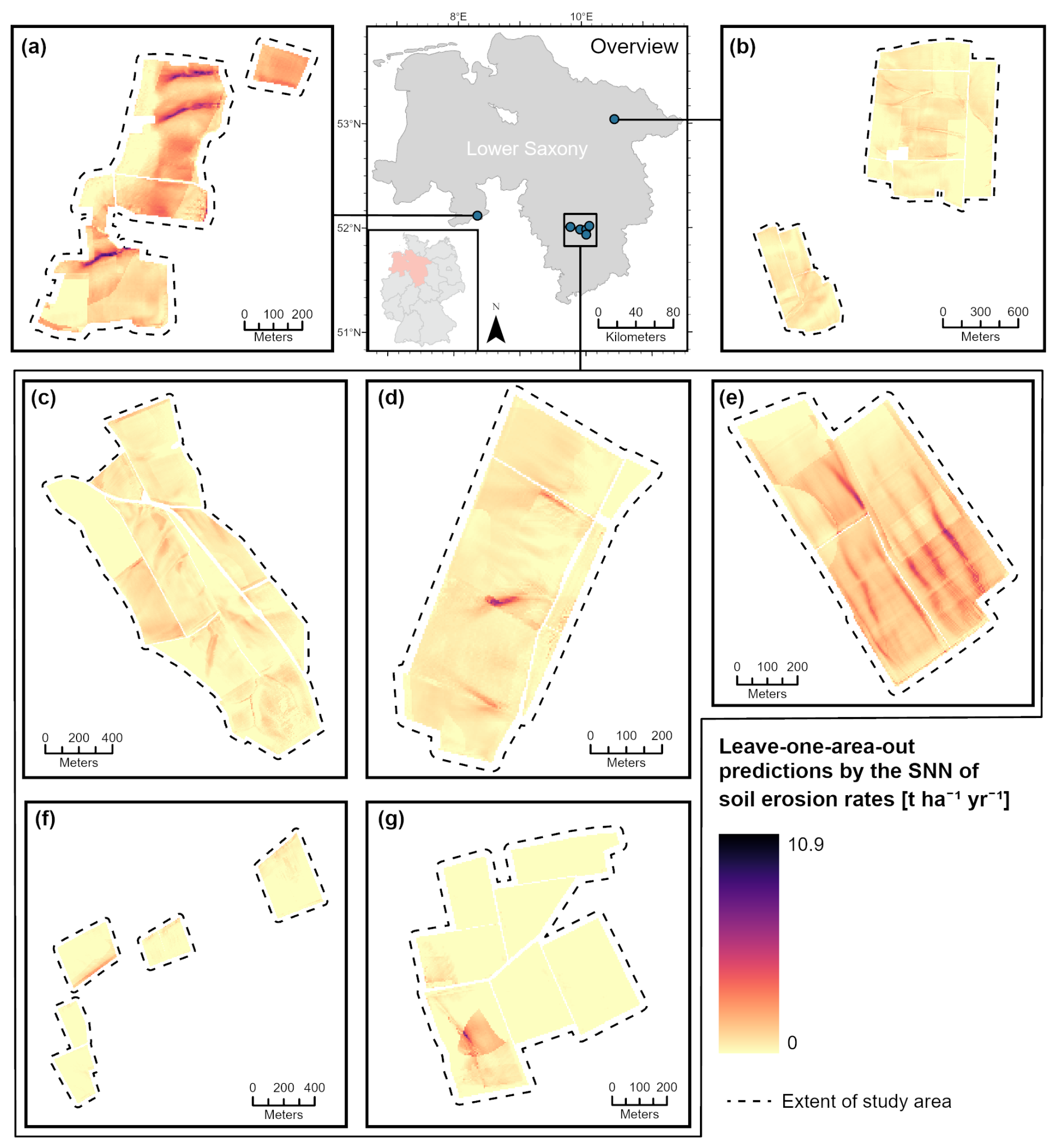
Figure C2 Predicted soil erosion rates using the leave-one-area-out approach by the single-hidden layer neural network (SNN) in (a) Küingdorf, (b) Barum, (c) Lamspringe, (d) Klein Ilde, (e) Nette, (f) Adenstedt and (g) Brüggen.

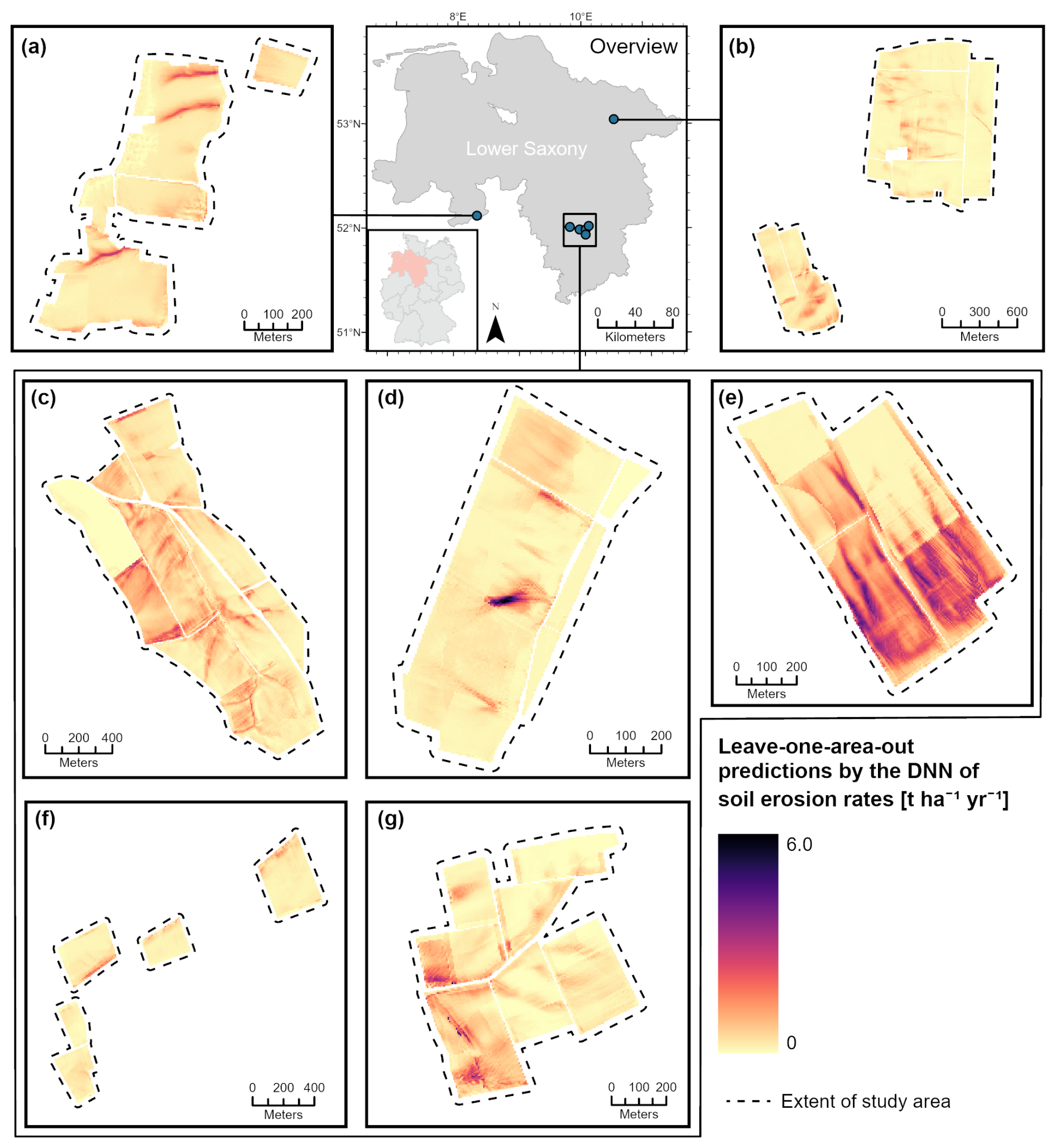
Figure C3 Predicted soil erosion rates using the leave-one-area-out approach by the deep neural network (DNN) in (a) Küingdorf, (b) Barum, (c) Lamspringe, (d) Klein Ilde, (e) Nette, (f) Adenstedt and (g) Brüggen.

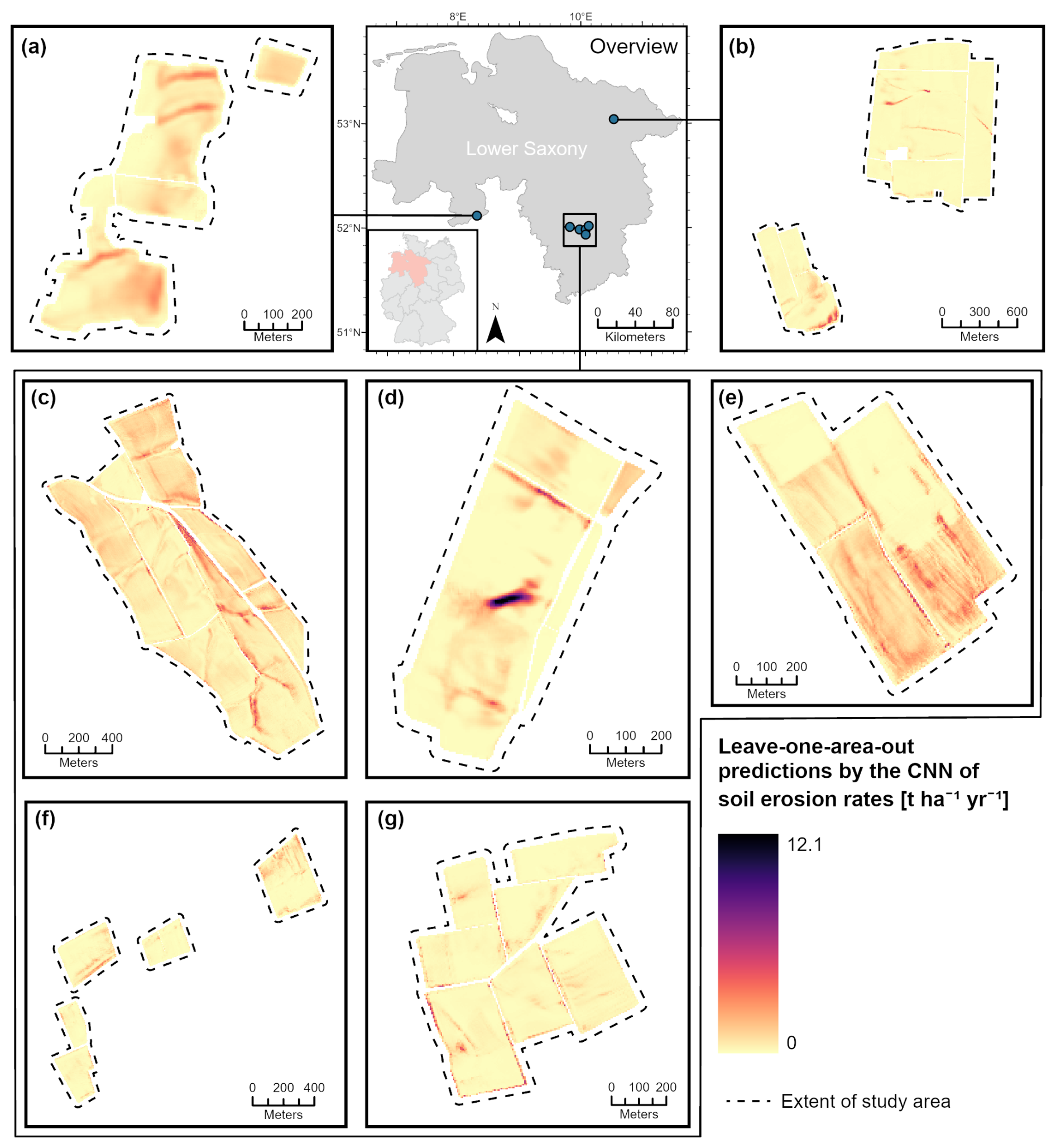
Figure C4 Predicted soil erosion rates using the leave-one-area-out approach by the convolutional neural network (CNN) in (a) Küingdorf, (b) Barum, (c) Lamspringe, (d) Klein Ilde, (e) Nette, (f) Adenstedt and (g) Brüggen.

C2 Differences between predicted and mapped soil erosion rates

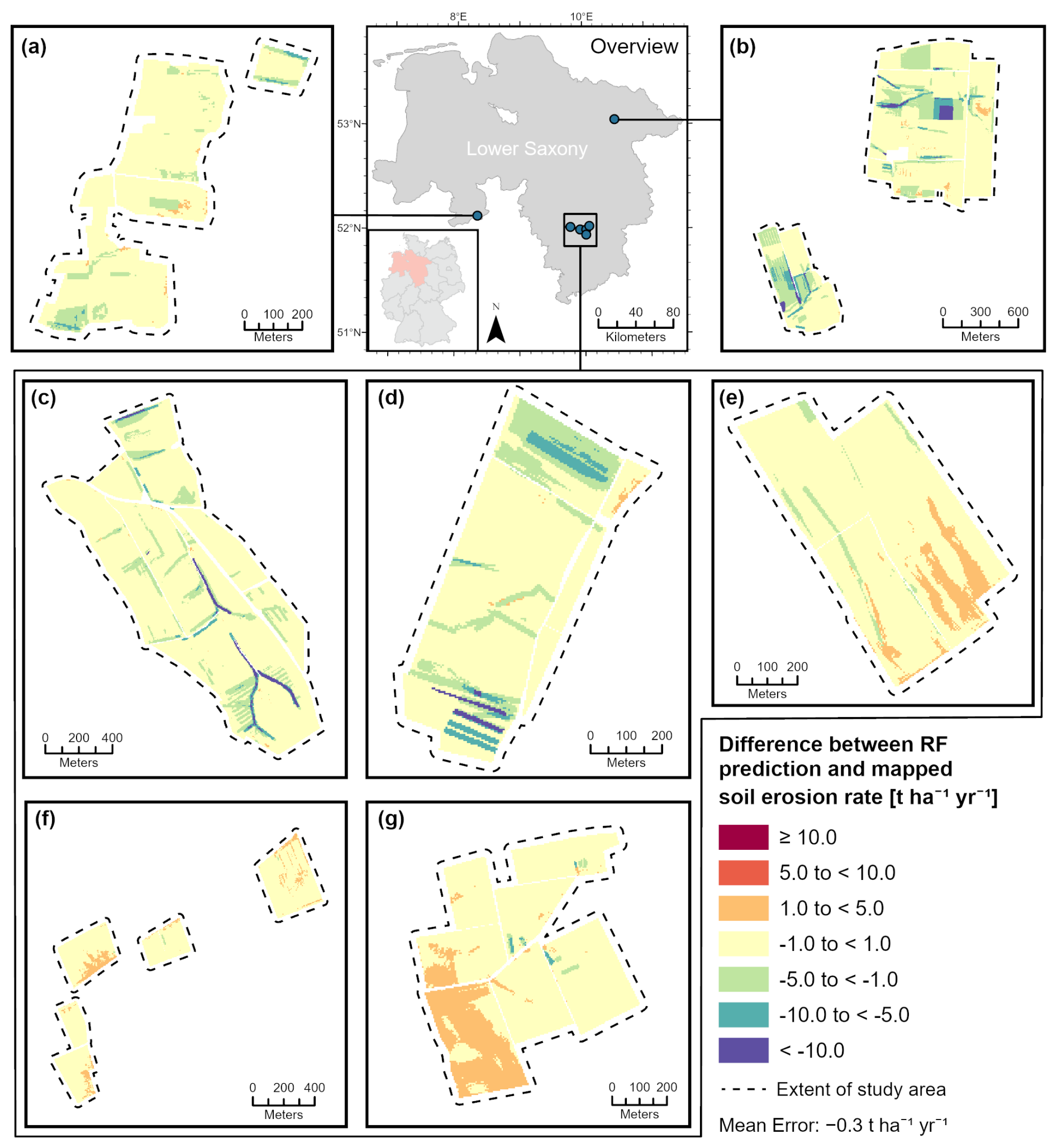
Figure C5 Difference between soil erosion rates predicted by the random forest (RF) and the mapped values in (a) Küingdorf, (b) Barum, (c) Lamspringe, (d) Klein Ilde, (e) Nette, (f) Adenstedt, and (g) Brüggen, where positive values indicate overestimation of the model and negative values indicate underestimation.

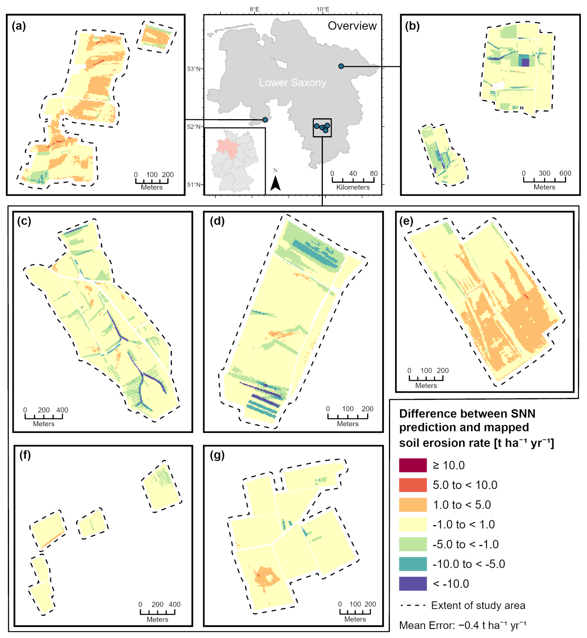
Figure C6 Difference between soil erosion rates predicted by the single-hidden layer neural network (SNN) and the mapped values in (a) Küingdorf, (b) Barum, (c) Lamspringe, (d) Klein Ilde, (e) Nette, (f) Adenstedt, and (g) Brüggen, where positive values indicate overestimation of the model and negative values indicate underestimation.

Figure C7 Difference between soil erosion rates predicted by the deep neural network (DNN) and the mapped values in (a) Küingdorf, (b) Barum, (c) Lamspringe, (d) Klein Ilde, (e) Nette, (f) Adenstedt, and (g) Brüggen, where positive values indicate overestimation of the model and negative values indicate underestimation.

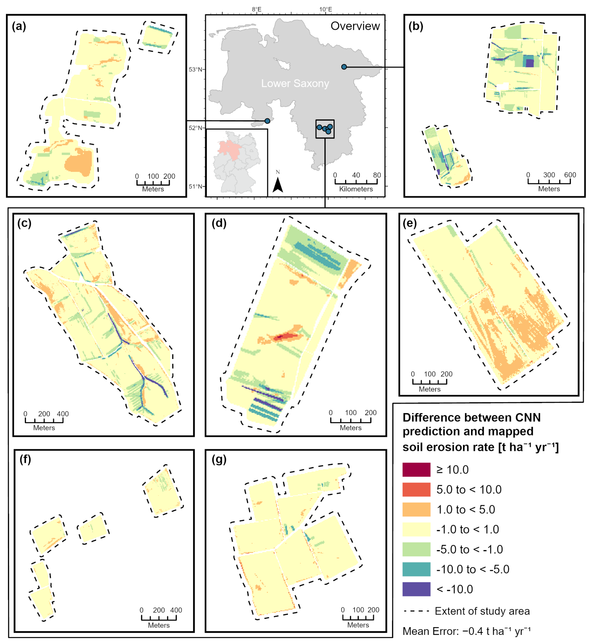
Figure C8 Difference between soil erosion rates predicted by the convolutional neural network (CNN) and the mapped values in (a) Küingdorf, (b) Barum, (c) Lamspringe, (d) Klein Ilde, (e) Nette, (f) Adenstedt, and (g) Brüggen, where positive values indicate overestimation of the model and negative values indicate underestimation.

Table C1 Per-study-area summary statistics of mapped soil erosion rates and model predictions (in t ha⁻¹ yr⁻¹) from the random forest (RF), single-layer neural network (SNN), deep neural network (DNN), and convolutional neural network (CNN).