High-resolution frequency-domain electromagnetic mapping for the hydrological modeling of an orange orchard

While aboveground precision agriculture technologies provide spatial and temporal datasets that are ever increasing in terms of density and precision, belowground information lags behind and has been typically limited to time series. As recognized in agrogeophysics, geophysical methods can address the lack of subsurface spatial information. This study focuses on high-resolution frequency-domain electromagnetic induction (FDEM) mapping as an ideal complement to aboveground and belowground time series that are commonly available in precision agriculture. Focused on a Sicilian orange orchard, this study first investigates some methodological challenges behind seemingly simple FDEM survey choices and processing steps, as well as their interplay with the spatial heterogeneity of agricultural sites. Second, this study shows how the detailed FDEM-based spatial information can underpin a surface/subsurface hydrological model that integrates time series from soil moisture sensors and micro-meteorological sensors. While FDEM has long been recognized as a promising solution in agrogeophysics, this study demonstrates how the approach can be successfully applied in an orchard, whose 3D subsurface variability is a complex combination of root water uptake, irrigation, evapotranspiration, and row–interrow dynamics. The resulting hydrological model reproduces the observed spatiotemporal water dynamics with parameters that agree with the results from soil laboratory analysis, supporting gamma-ray and electrical resistivity tomography datasets. The implementation of a hydrological model positively aligns with the increasing number and variety of methods in precision agriculture, as well as with the need for better predictive capability.

1 Introduction

Precision agriculture, a management strategy for addressing spatial and temporal variabilities in agricultural fields that involves data and contemporary technologies, directly points at both spatial mapping and temporal monitoring technologies (McBratney et al., 2005). Remote sensing, the Internet of Things, big data, and artificial intelligence drove and drive significant advances in the monitoring and management of aboveground variables and agricultural practices (Karunathilake et al., 2023). On the contrary, the understanding of the subsurface spatiotemporal variability lags behind, hindered by open methodological challenges and, consequently, limited information availability.

With regard to the subsurface, soil sensors remain the foremost driver of precision agriculture (Shafi et al., 2019). These sensors provide high-resolution temporal information on key soil state variables, such as volumetric water content (VWC), water potential, heat flux, and temperature (Yu et al., 2021; Kustas et al., 2000; Tuzet et al., 1997). However, their limited spatial representativeness and high sensitivity to local and installation factors are well-known issues (Vereecken et al., 2016; Rivera et al., 2012; Everett and Chave, 2019; Evett et al., 2008). Cosmic-ray neutron sensing is a newer technology that addresses some of these issues, with the water content information being integrated over an areal footprint with a radius of several tens of meters (Zreda et al., 2008; Li et al., 2019). In this sense, however, the integrated VWC remains limited to a one-dimensional time series and does not provide direct information on the spatial variability as the measured VWC is averaged over the footprint area and a thickness of a few tens of centimeters. A second concern with cosmic-ray neutron sensing is the penetration depth being limited by the physical process and soil conditions, which can be modeled but not controlled (Köhli et al., 2015). This aspect becomes particularly relevant when targeting deeper root water uptake (RWU), for example, beyond 50 cm depth in orchards. Overall, the combination of soil sensors and cosmic-ray neutron sensing allows for the monitoring of temporal variability but fails to capture spatial variability with adequate spatial resolution (Vereecken et al., 2007, 2008; Binley et al., 2015).

The use of geophysics has been explored to address this key and open issue, e.g., as in Garré et al. (2021) and Binley et al. (2015). Among geophysical methods, electrical resistivity tomography (ERT) and frequency-domain electromagnetic induction (FDEM) are used for their sensitivity to water content, water salinity, and relevant soil properties (O'Leary et al., 2024; Rubin and Hubbard, 2005). These methods can target the spatiotemporal water dynamics induced by irrigation and evapotranspiration (ET), including at depths where soil sensors are difficult to install and where cosmic-ray neutron sensing has limited sensitivity. ERT and FDEM primarily measure the electrical resistivity of the subsurface while also being sensitive to its capacitive and inductive response (Rubin and Hubbard, 2005). ERT relies on the galvanic injection of electrical current and measurement of the associated distribution of the electric field to image the variability of the electrical resistivity. FDEM uses solenoids to induce and measure the electromagnetic induction response of the subsurface, with no direct contact. From the measured electrical resistivity, the relevant hydrological properties are then qualitatively or quantitatively derived through petrophysical relationships or the calibration of hydrogeophysical models (Wagner and Uhlemann, 2021; Boyd et al., 2024), RWU (Blanchy et al., 2020a; Mary et al., 2021), and ET (Dumont and Singha, 2024; Chou et al., 2024; Peruzzo et al., 2024).

In recent years, progress has been made in the FDEM-based study of the intra-field variability and soil–plant correlations at the scale of a few meters (Boaga, 2017). This scale suitably addresses the soil spatial variability and its impact on irrigation and vegetation, especially in crop farming (O'Leary et al., 2024; Von Hebel et al., 2021). On the contrary, methodological challenges hindered the possibility of resolving strong spatiotemporal complexity at smaller scales (Blanchy et al., 2024; Carrera et al., 2024; Klose et al., 2022). These small-scale spatiotemporal variabilities are associated with irrigation and RWU–ET dynamics in orchard farming and thus are central to agroecosystems and precision agriculture (Galindo et al., 2018; Yang et al., 2022). ERT has been applied to the meter and sub-meter scales thanks to its spatial flexibility in terms of scale and resolution (Cassiani et al., 2015, 2016; Watlet et al., 2024). Applications have successfully imaged and monitored the RWU dynamics of crops (Michot et al., 2003; Beff et al., 2013; Boaga et al., 2014; Garré et al., 2011; Gu et al., 2025) and fruit trees (Mary et al., 2018; Mary, 2020; Peddinti et al., 2018; Vanella et al., 2018, 2021). In general, these ERT setups showed how ERT successfully addresses the need for high-resolution and time-lapse measurements (Blanchy et al., 2025; Mary et al., 2023; Peruzzo et al., 2020). Hence, ERT is often used to provide specific details supporting the interpretation of the FDEM results (Blanchy et al., 2020b). In turn, the FDEM results can guide the ERT surveys and upscale their results (Carrera et al., 2024; McLachlan et al., 2017) and provide a link with remote-sensing data (Von Hebel et al., 2021; Hubbard et al., 2021).

The above geophysical studies have shown how FDEM and ERT are particularly suitable for targeting water spatiotemporal dynamics, including irrigation strategies, RWU, and ET. Over the last few decades, there has been extensive research into irrigation optimization, often in the frame of regulated deficit irrigation, and other soil and water conservation strategies. The proposed optimizations require careful understanding and monitoring of the ET and RWU dynamics (Fereres and Soriano, 2006). Differently, the desired moderate water stress becomes too severe and causes negative physiological and yield consequences (Chai et al., 2016). This optimization faces critical methodological challenges with regard to how soil heterogeneity and ET changes affect the irrigation-ET balance. For example, variable soil thickness and texture impact the water dynamics and become critical for timing the irrigation inputs (Patzold et al., 2008). Yang et al. (2022) indicated the lack of consensus regarding suitable irrigation systems and procedures, i.e., rather practical aspects related to the water dynamics, as a key adoption problem for regulated deficit irrigation. Beyond the short-term management of irrigation, a better understanding of the RWU also underpins the evaluation of long-term morphological and physiological responses of crops to irrigation changes (Saitta et al., 2021; Maurel and Nacry, 2020).

In orchard farming, the presence of significant row–interrow differences further increases the spatial complexity. The use of soil water sensors and cosmic-ray neutron sensing becomes particularly problematic when investigating the interplay of different treatments, genotypes, and water deficits as their time series cannot be upscaled or generalized (Vanella et al., 2025). Jovanović et al. (2023) investigated the row-interrow water dynamics in a Japanese plum orchard, including 2D numerical simulations (HYDRUS-2D). While the calibrated model successfully reproduced the measured ET time series, the discussion of the 2D water dynamics was ultimately limited by the absence of spatial information for the subsurface. Similarly, Searles et al. (2009) studied the adaptation of the root system of olive trees to different drip irrigation systems based on soil auger samples. The results provided significant statistics on the root morphology but also highlighted the intrinsic limitations of samples with regard to root functioning and water spatiotemporal dynamics. In this sense, Vanella et al. (2022) successfully proposed the use of time-lapse ERT measurements to target spatiotemporal water changes in an almond orchard and discussed the variable agreement with FDEM surveys and cosmic-ray neutron fluxes. More generally, the complexity of water dynamics supported the increasing integration of geophysical data and other hydrological datasets. This integration is central to hydrogeophysics and can follow different approaches (Rubin and Hubbard, 2005; Binley et al., 2015; Uhlemann et al., 2024), including coupled and uncoupled hydrogeophysical modeling (Rossi et al., 2015). The implementation of hydrological models is also motivated by the general need for validation and prediction (Beven, 2008; Ward et al., 2018), especially for precision agriculture in sensitive areas under climate change (Lakhiar et al., 2024; Fan et al., 2017; Behnassi et al., 2024).

As introduced above, the increasing number of studies that explored hydrogeophysical integration largely relied on ERT surveys because of advantageous spatial scale flexibility and monitoring capabilities. Nonetheless, FDEM has been presented as the ideal solution to fully match the large area and spatial variability of agricultural sites. This study first explores the methodological challenges that hinder high-resolution FDEM characterizations of the strong spatial variability associated with irrigation and ET dynamics, especially in orchards. Our first hypothesis is that these challenges are not sufficiently recognized or discussed and that the complexity behind seemingly simple survey choices and processing steps limits the FDEM technological readiness and applications in agrogeophysics. We worked in a Sicilian orange orchard where ultra-low drip irrigation is applied, collecting several FDEM datasets with different instruments, coil orientations, and coil heights. The direction and spacing of the survey lines were also varied to investigate the effect of the field anisotropy associated with tree and irrigation lines. Three time-lapse ERT datasets were collected and used to support the FDEM results. Next, this study investigates how addressing these challenges allows for an effective coupling between temporal information from the widely used soil water sensors and spatial information from FDEM mapping. A second hypothesis is that this combination can suitably inform conceptual hydrological models that are sufficiently detailed to capture the relevant spatiotemporal complexity but also cover entire plots or large areas, e.g., extending common ERT applications. Third, the derived conceptual model was used to implement a 3D (CATHY) numerical model that includes both soil water dynamics (RWU and irrigation) and ET (Camporese et al., 2010, 2014). Beyond the validation of the conceptual model, this last step is aimed toward agrogeophysical studies that include both subsurface and surface hydrology, as well as hydrological models. The third hypothesis is that the assimilation of soil sensors, FDEM mapping, and micro-meteorological data can constrain a realistic surface and/or subsurface hydrological model. This last step is a fundamental step forward in the direction of the most fundamental spirit of “hydrogeophysics” that resides in the integration of geophysical data as further and often fundamental experimental evidence to be compared against modeling predictions, thus closing the loop in the scientific reasoning in developing a validated (non-falsified) conceptual model of the system, to be used for predictions and actual practical purposes.

2 Materials and methods

The experiments were conducted in a 20 ha orange farm located in Lentini (eastern Sicily; 37°20^′24^′′ N, 14°53^′33^′′ E; WGS84) in a Mediterranean semi-arid environment. The topography of the farm is flat. The farm is managed by Centro di Ricerca Olivicoltura, Frutticoltura e Agrumicoltura of the Italian Council for Agricultural Research and Agricultural Economics Analyses (CREA-OFA). The annual average precipitation is around 573 mm, with very dry summers and average air temperatures of 7 °C in winter and 28 °C in summer (years from 2002 to 2023). The investigated subplot was planted in 2021 with 3-year-old orange trees. The trees were planted in eight parallel rows that were 100 m long. The tree rows were spaced 6 m apart, and the tree interspacing along each row was 4 m. The trees had a height of 88±41 cm, a crown diameter of 79±24 cm, and a stem diameter of 3.7±0.8 cm (measurements refer to the time of the study, namely June 2023; the indicated ranges are standard deviations and reflect the real variability of the trees, i.e., not the uncertainty of the measurements).

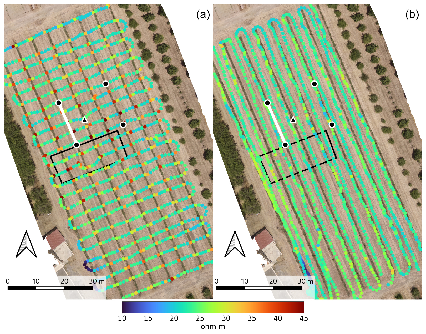
Figure 1 GEM-2 survey over the entire plot area. The shown apparent resistivities were measured at 5325 Hz and investigate the water distribution in the deeper region, dominated by the RWU. Panel (a) shows the transversal dataset that captures the variability between the tree lines – drier and thus more resistive because of the RWU – and the more conductive interrows. In (b), the longitudinal dataset shows intermediate values, having the tree lines on one side and the interrow on the other. The black dots indicate the position of the soil sensors. The black triangle indicates the position of the net radiometer. The rectangular black perimeter shows the FDEM's high-resolution inverted region. The white segment represents the ERT section. The background is a reconstructed RGB orthophoto mosaic.

An ultra-low drip irrigation system was designed and installed by Irritec, made of three independent drip lines along each tree row (Irritec P5, 16 mm of diameter). Along each drip line, the drip spacing was 0.5 m. Two of the drip lines had drippers with a flow rate of 0.8 L h⁻¹. The third drip line had drippers with a flow rate of 0.6 L h⁻¹. The three drip lines result in an irrigation of 4.4 L m⁻¹ h⁻¹ along the tree rows (at the full irrigation rate), distributed over a strip with a width of 1 m. Focusing on the experiment subplot, the irrigation lasts, on average, 5 h, typically from 06:00 to 11:00 LT. The irrigation provides about 2850 L over an area of about 24 m × 33 m. The irrigation input is calculated from the pressure-regulated drippers and is periodically confirmed by monitoring the water inputs from selected drippers. The irrigation schedule maintains good soil water potential conditions – between field capacity (FC) and permanent wilting point (WP) – throughout the year.

Four VWC sensors (Teros 10 by METER Group) and soil heat flux plates (HFP01-05 by Hukseflux) were installed in 2021 and maintained throughout the 2023 growing season (Fig. 1). The sensors were installed along two tree rows (Fig. 1), with the VWC sensors being installed at a depth of 20 cm and the soil heat flux plates being installed at a depth of 5 cm. A net radiometer was installed at approximately the center of the subplot (Fig. 1). Additional agrometeorological data (air temperature, air humidity, wind speed, and rainfall) were monitored by an automatic weather station located about 2 km from the orchard and managed by the Agrometeorological Service of the Sicilian Region. All of the time series were homogenized to hourly data and daily averages (Vanella et al., 2025).

Eight samples were collected to measure the VWC at FC (−0.3 kPa) and WP (−15 kPa). The obtained values were used to determine the water retention properties of the soil and to calibrate the VWC time series from the soil sensors. While the Teros 10 sensors are standard and reliable sensors, calibration procedures are known to improve their accuracy (Cominelli et al., 2024). Because of the specific irrigation schedule and long-term research studies at the site, the field VWC is known to vary between FC and WP. Hence, the laboratory VWC values were used to rescale the time series recorded by the field sensors.

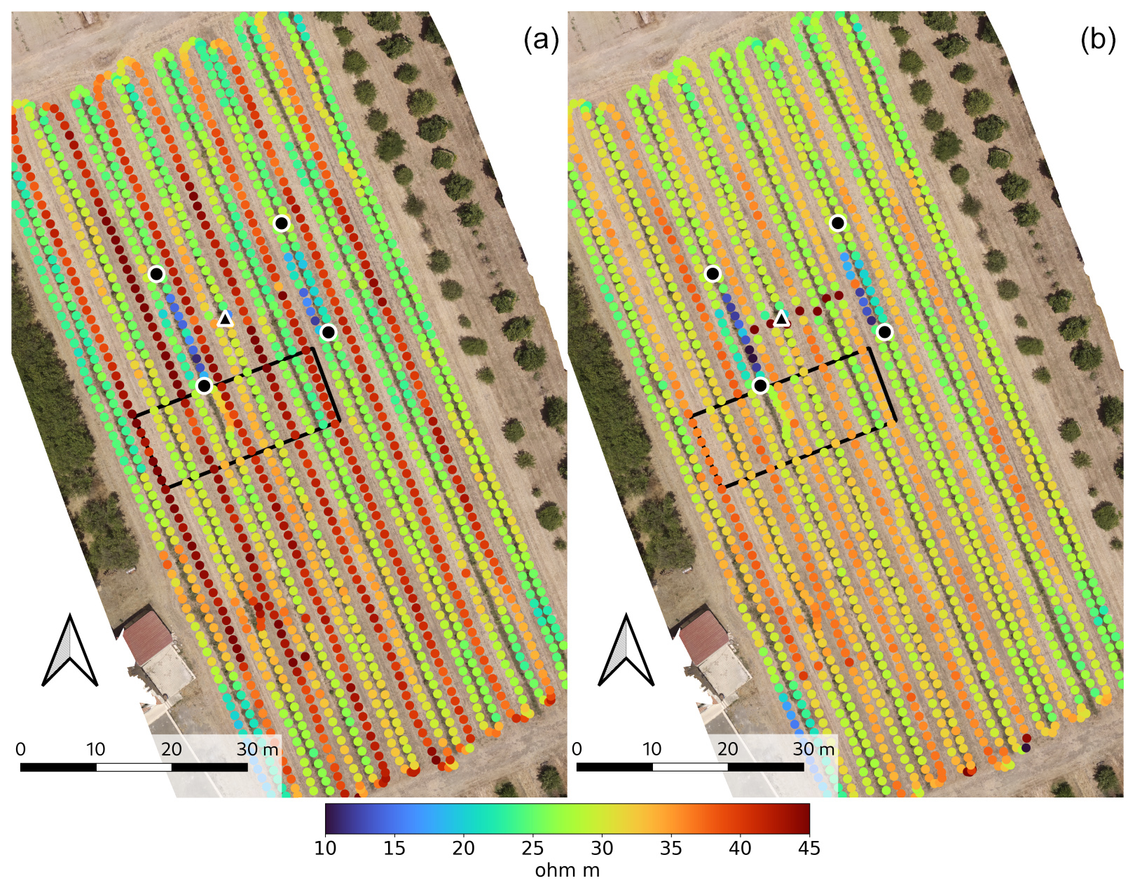
Figure 2 Mini-Explorer survey over the entire plot area using the horizontal coplanar configuration. The two datasets show how the water content and, thus, the resistivity distribution become smoother with increasing depth. In (a), the 0.71 m coil separation dataset distinctly shows the dry interrow, exposed to evaporation without significant irrigation recharge. In (b), the 1.18 m coil separation dataset shows a smoother transition from the tree lines to the interrow, which is less directly exposed to evaporation.

2.1 Geophysical measurements

The field measurements were conducted on 28 June 2023, a clear-sky day with a maximum air temperature of 36 °C. The described irrigation schedule was applied in the morning, from 06:00 to 11:00 LT, with a total input of 2850 L over the four tree rows. Five FDEM surveys were carried out at the end of the irrigation, from 11:00 to 14:00 LT, using a Geophex GEM-2 and a CMD Mini-Explorer. The GEM-2 is a multi-frequency instrument with a fixed coil separation of 1.66 m that uses multiple frequencies to vary the investigation depth (Blanchy et al., 2024; Deidda et al., 2023). In this study, the GEM-2 was set to measure at 425, 1525, 5325, 18 325, 63 025, and 92 775 Hz. The Mini-Explorer is a multi-coil instrument with three coil separations of 0.32, 0.71, and 1.18 m, operating at a fixed frequency of 30 kHz (Bonsall et al., 2013). The FDEM surveys were carried out with the instruments at a height of 0.1 m. Three surveys were collected with the GEM-2: two surveys covered the entire plot, one was parallel to the tree lines, one was transversal to the tree lines, and one focused on a selected sub-area with a finer spatial resolution and both surveying directions (Fig. 1). The remaining two surveys were collected with the Mini-Explorer: one covered the entire plot, only parallel to the tree lines, while the second survey focused on the same high-resolution area (Figs. 2 and 3). A GPS (Hemisphere GPS A101 Smart Antenna) with RTK correction was used with the Mini-Explorer, while a smaller GPS receiver was installed directly on the GEM-2 and had no RTK correction. During the survey, known positions (e.g., ends of tree rows) were marked to allow for the control and, possibly, to correct the GPS coordinates. In addition to the above five datasets, two initial GEM-2 surveys were conducted at an instrument height of 0.9 m above the ground to test the instrument sensitivity at different heights. However, these two initial datasets are only considered for the methodological part because they capture neither the irrigation nor the ET (due to their limited resolution depth).

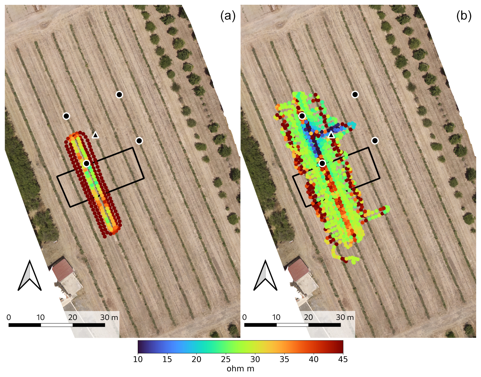
Figure 3 (a) Mini-Explorer (0.32 m coil spacing, horizontal coil orientation) and (b) GEM-2 (18325 Hz, horizontal coil orientation) surveys over the high-resolution area, overlapping with the inversion region. While both datasets present longitudinal resistive strips, the Mini-Explorer detects the shallow evaporation, while GEM-2 senses the deeper RWU. Both transpiration and RWU are captured and represented by multiple data points thanks to the denser spatial sampling (i.e., smaller gaps between the survey lines).The rectangular black perimeter shows the FDEM high-resolution inverted region.

The FDEM datasets were processed and inverted using Python and EMagPy (QGIS Development Team, 2024; Van Rossum and Drake, 2009; McLachlan et al., 2021). The datasets were initially imported into EMagPy to obtain the correct apparent conductivities, taking into account the relevant survey parameters. The GEM-2 quadrature outputs were converted into apparent conductivities, and the Mini-Explorer apparent conductivities were recalculated to correct the default factory conversion. The latter Mini-Explorer adjustment starts by removing (i.e., dividing by) the numerical factor defined by the manufacturer for the default conversion from quadrature to apparent conductivities and then uses the quadrature values in EMagPy to numerically calculate the apparent conductivities, with the correct surveying parameters. No smoothing or filtering was applied during this initial step. The corrected apparent conductivities were then exported and further processed in QGIS, starting from the correct positioning. First, the correctness of the GPS coordinates was verified by comparing the relative positions of the datasets and the absolute position based on a high-resolution orthophotograph of the site. The individual datasets were georeferenced with respect to known survey locations when necessary. Second, the data quality of the individual datasets was evaluated by observing the values of the apparent conductivity and their distribution. In some cases, the data appeared to be void of relevant information and thus were dismissed. This was the case for the two GEM-2 datasets acquired at 0.9 m elevation and for the two lowest frequencies of the other GEM-2 datasets (see Results and Discussion sections). Repeated measurements at the same location were compared to verify possible instrumental drift. The processed datasets were then merged by interpolating all the datasets over a common grid. A 2D kriging interpolation was performed to properly account for the site anisotropy, i.e., the periodicity and direction of the tree lines, as well as their inter- and intra-line tree spacing. Finally, the interpolated apparent conductivities were inverted using EMagPy with a linearized full-Maxwell forward model and a Gauss–Newton optimization method. The inversion model was defined with 24 layers of increasing thickness downward, from 5 cm at the surface to 30 cm at a depth of 2.6 m. Layer thicknesses and maximum depth were chosen based on sensitivity profiles calculated with EMagPy (Fig. 4).

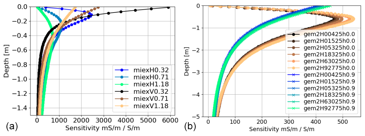
Figure 4 Sensitivity profiles of the Mini-Explorer (a) and GEM-2 (b). In (a), both horizontal (H) or vertical (V) coplanar orientations are simulated for the Mini-Explorer. The legend describes the coil orientation and their spacing (m). In (b), the GEM-2 horizontal (H) coil orientation is shown for the different measurement frequencies (Hz) and two heights of the instrument (m). All sensitivities were calculated with a homogeneous model of 10 mS m⁻¹ and 250 layers. The sensitivity profiles were not normalized by their maximum value but were normalized by the layer thickness (Deidda et al., 2023; Von Hebel et al., 2019).

An algorithm was developed to correct the possible off-center position of the GPS relative to the instrument footprint. The following steps were implemented in Python. After removing the GPS outliers or null positions, the coordinates were converted into UTM to ease the geometrical calculations. The step-wise changes in longitude and latitude were calculated between consecutive positions in order to position accurately the center of the FDEM coil pairs, starting from the actual position of the GPS antenna. While this may seem irrelevant for other studies, it proves to be crucial for precision measurements in this context. The step-wise moving angle was calculated from the step-wise changes using the arctangent function, and the standard atan2 function was used (Harris et al., 2020). A suitable time window was defined for the calculation of the mean moving angle and associated standard deviation (e.g., 2 s). Over the defined time window, the mean moving angle was calculated as the sum of the sine and cosine components of the step-wise moving angles, i.e., with the correct wrapping between 360 and 0°. The associated standard deviation of the moving angles was also calculated over the time windows. An estimate of the off-center error and needed correction length was defined based on the initial data visualization, e.g., 0.75 m. The longitude and latitude corrections were calculated by multiplying the sine and cosine of the moving angle by the defined correction length. The calculated corrections were added to the original coordinates. Relative to a comparison between the first and last point within the time window, the calculation of the average moving angle from the step-wise angles is statistically more robust and also yields the associated standard deviation. The standard deviation can be used to determine whether the estimated moving angle is sufficiently reliable to apply the correction.

Three high-resolution ERT datasets were acquired along a tree row to support the FDEM investigation of the water dynamics (Figs. 1 and 3). Hence, 72 electrodes were installed with an electrode spacing of 20 cm. The resulting section had a total length of 14.2 m, and it was located between the two western soil sensors, just north of the FDEM inversion area (Fig. 1). The three datasets were acquired at 11:30, 12:00, and 13:00 LT, i.e., overlapping with the FDEM surveys. Note that the high-resolution FDEM data were collected right after the ERT to maximize their representativeness while avoiding the possible effects of the ERT equipment. A dipole–dipole skip-two sequence with 5097 quadrupoles was used in line with the relatively short electrode array and desired high-resolution imaging. The sequence included all reciprocal measurements, which were used to estimate the data quality and the suitable data error for the ERT inversion. A threshold of 5 % of reciprocal error was used to filter the data prior to inversion. The retained data were then inverted using the same 5 % as the estimated error.

Gamma-ray spectroscopy was carried out using a Gamma Surveyor Vario VN6, by GF Instruments, to support the characterization of the soil texture. The spectrometer uses an NaI(Tl) detector and has 2048 channels, which allows separate measurements of the potassium (K), uranium (U), and thorium (Th). The gamma-ray decays were counted over a time period of 180 s. Ten evenly distributed measurements were collected over the orange orchard during the FDEM surveys. The concentrations of K, U, and Th were used as proxies for the content of clay and organic matter (Omoniyi et al., 2013; Dierke and Werban, 2013; Priori et al., 2013; Chiozzi et al., 2002). See Ahmad et al. (2019) and Rouze et al. (2017) for recent investigations of the correlations between soil composition and gamma response, especially K and clay content.

2.2 Hydrological model

A hydrological model based on CATHY (Camporese et al., 2010) was constructed from the geophysical spatial information, VWC time series from the soil sensors, and other supporting information. CATHY is a physically based model that solves the coupled equations for the surface and subsurface flow in saturated and unsaturated conditions. CATHY implements the physical processes that are central to the current study. A plant physiology model allows for a refined control of the RWU as a function of depth and soil water potential (Feddes et al., 1976, 2001; Camporese et al., 2015). A boundary condition switch allows for a good description of the ET dynamics, which are either controlled by the atmosphere (net radiation) or limited by soil when the water suction exceeds a certain threshold (Camporese et al., 2014). Water input and ET can vary in both space and time, which allows the simulation of the described irrigation schedule and the row–interrow ET spatial differences.

The model domain measures 18 m × 2 m, and it is perpendicular to the tree lines. Given the tree row spacing of 6 m, the length of 18 m covers two tree rows, with their shared interrow at the center of the model. The model depth was set to 5 m to exceed the depth of the water dynamics and the measurement sensitivities. The soil surface was assumed to be flat over the entire area. The model was horizontally discretized with 10 cm wide cells. A total of 15 layers were defined for the vertical discretization, with their thickness increasing downward from 10 cm to 1 m (La Cecilia and Camporese, 2022). The RWU differences between the rows of orange trees and the interrow were expressed by adjusting their Feddes parameters (Feddes et al., 1976, 2001). For the orange trees, the maximum rooting depth was set to 2 m but with RWU being at its maximum within the first meter (Hou et al., 2023; Cassiani et al., 2015; Morgan et al., 2007). For the grass, the maximum rooting depth was set to 0.2 m, with RWU decreasing linearly from the soil surface. The other RWU parameters were kept equal for orange trees and grass: WP at −15 kPa, deficit point at −10 kPa, and anaerobiosis point at −1 kPa. RWU compensation was included for both orange trees and grass, which allows the model to adjust the RWU profile according to the water stress profile (Camporese et al., 2015).

The irrigation was modeled by distributing the known water inputs over two stripes of 1 m width along the two tree rows. This resulted in a water input of $\mathrm{1.22}\times {\mathrm{10}}^{-\mathrm{6}}$ m s⁻¹ over the 5 h of irrigation, i.e., reproducing both flow rates and schedule of the irrigation system described above. A period of 14 d was simulated to cover three irrigations, with the third irrigation corresponding to the day of the geophysical measurements. The 2-week period and the two previous irrigations were simulated to realistically equilibrate the model (e.g., VWC distribution) before the day of the measurements. The soil hydraulic properties were parameterized using the Mualem–van Genuchten model and the saturated hydraulic conductivity, with initial parameter values being derived from the water retention experiment performed in the laboratory (1500F1 Pressure Plate Extractor by SoilMoisture Equipment Corp) and considering the soil texture information (Mualem, 1976; van Genuchten, 1980). The ET was defined through a time series of potential ET, expressing the atmospheric forcing to which the surface (soil and vegetation) responds accordingly to water availability. The potential ET was based on the data measured by the local weather station and eddy covariance tower, in line with studies conducted in the area (Vanella et al., 2025; Mary et al., 2019). No rain inputs were simulated because the weather remained stable and sunny during the simulation period, and no rain was measured by the local rain gauge. Geophysical spatial information and soil VWC time series were combined to constrain the soil parameters values and, thus, the water spatiotemporal dynamics. The other model inputs (e.g., potential ET, irrigation inputs) were known from measurements and, thus, were fixed as boundary conditions.

3 Results

The FDEM apparent conductivities, pre-processed and exported from EMagPy, were visualized over the site orthophoto. The data quality was generally good and allowed for the desired mapping over the entire investigated area. However, some GPS corrections were needed before examining the FDEM data. The GPS coordinates of the GEM-2 data were affected by both variable GPS errors (up to 2 m in some instances) and systematic off-centering of the GPS relative to the instrument footprint (Choi and Kim, 2020). The errors were very visible and relevant because of the known survey geometry imposed by tree lines. The off-centering caused the high apparent resistivity (ρ_a) values in Fig. 1a, corresponding to the tree lines, to shift eastward of about 0.75 m when walking eastward and vice versa when walking westward, for a combined shift of about 1.5 m. The described GPS-centering algorithm successfully corrected the off-center errors and thus realigned the survey lines. Similarly, the marked survey locations allowed for the correction of time-variable (variable in time) GPS errors with the QGIS georeference tools.

Of the six GEM-2 survey frequencies, the lowest two (425 and 1525 Hz) were discarded because of a very low signal-to-noise ratio, which resulted in very unstable and often negative apparent conductivities. The data quality increased significantly at higher frequencies. Figure 1 shows the GEM-2 data measured at 5325 Hz over the entire field. The two GEM-2 surveys (along and across the tree lines) agree on the measured ρ_a, ranging between 20–30 Ωm along the interrows. In addition, the transversal survey shows higher ρ_a values corresponding to the tree-irrigation lines, reaching values of 40–45 Ωm. While the spatial correspondence of tree lines and high ρ_a values is clear over the entire field, only one or two data points capture the resistive anomaly. The ρ_a values rapidly decrease on both sides of the tree lines. In fact, these higher values are not captured by the longitudinal survey, which was carried out along the tree irrigation lines but necessarily to their sides (about 1 m, Fig. 1). The other GEM-2 datasets, shallower because of the higher frequencies, also show larger values of resistivity along the tree irrigation lines but with smaller contrasts.

Figure 2 shows the Mini-Explorer data measured with the coil separations of 0.71 and 1.18 m in horizontal coplanar configuration, surveying longitudinally to the tree irrigation lines over the entire field. The ρ_a varies between 20 and 45 Ωm. The ρ_a changes are dominated by differences between the tree irrigation lines and their interrows, similarly to the GEM-2. However, the high ρ_a lines match the tree irrigation lines in the GEM-2 datasets and the center of the interrow in Mini-Explorer; i.e., high- and low-resistivity areas are inverted. Figure 2 also shows that the high ρ_a measured by the Mini-Explorer along the interrows decreases with increasing coil separation, from values of 45 to 35 Ωm. Consequently, the resistivity contrast between tree rows and interrows is larger in the shallower dataset. The dataset acquired with the shortest coil separation (0.32 cm) and the datasets acquired in vertical coplanar configuration align with this trend (see FDEM inversion below).

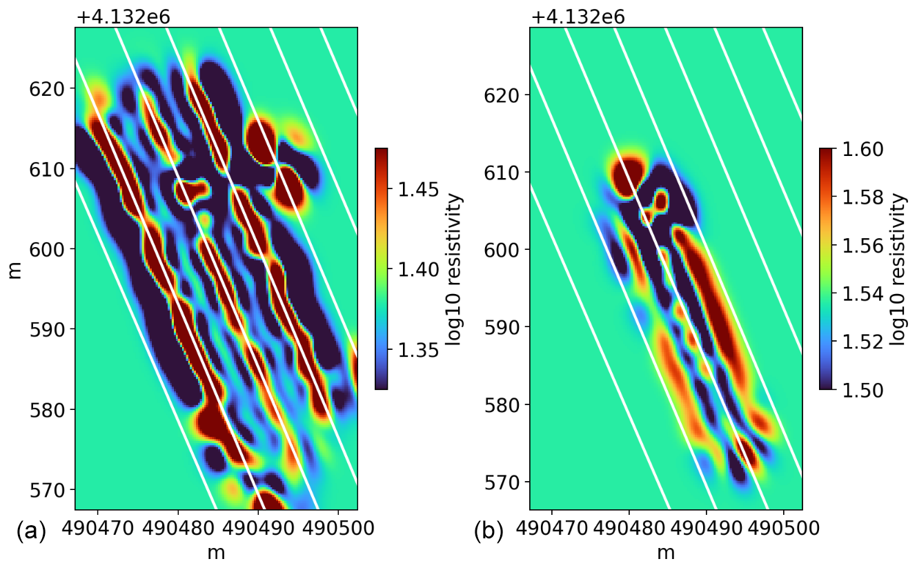
Figure 5 Interpolation of the high-resolution datasets (as ρ_a) acquired with (a) the GEM-2 at 92 775 Hz and (b) the Mini-Explorer with the coil separation of 1.18 m. Because of the high frequency and long coil separation (Fig. 4), the two datasets capture the intermediate depth and thus represent a connection between the GEM-2 and Mini-Explorer surveys. The GEM-2 survey captures well the resistive lines associated with the tree rows (white lines) but also shows a smaller increase in resistivity at the center of the interrow. Vice versa, the Mini-Explorer survey better captures the resistive lines along the interrows, with some smaller resistive anomalies matching the tree rows. The “secondary” resistive features within each survey required the high-resolution surveys, kriging interpolation, and narrow color ranges in order to be appreciated. The combination of the instruments allowed and guided this detailed investigation. The anomalous regions in the northern two-thirds of the maps correspond to the area affected by the wiring of the soil sensors (Fig. 3).

Figure 3 shows the FDEM surveys with a finer spatial resolution. Both GEM-2 and Mini-Explorer datasets show ρ_a values consistent with the respective larger-scale surveys. The better spatial sampling of both tree irrigation lines and interrows clarifies the transition between rows and interrows in the Mini-Explorer dataset. The resistive interrow appears to be wider and not only limited to the center of the interrow, as in the larger survey. The high-resolution Mini-Explorer survey also highlights the drop in ρ_a at the end of the Mini-Explorer longitudinal lines, when the acquisition pathways turn. The resulting intermediate ρ_a values are coherent with the footprint that becomes transversally elongated with respect to the tree rows and, thus, partially covers both tree rows and interrows. In the GEM-2 survey, more data points capture the resistive line associated with the tree row, again, better defining the width of the resistive line and excluding possible doubts regarding the reliability of individual data points. The high-resolution surveys reveal some secondary detailed spatial features that are missed by the larger surveys. Figure 5 shows how the deepest Mini-Explorer (1.18 m coil separation) and shallowest GEM-2 (92 775 Hz) surveys capture an intermediate condition in which both tree rows and interrow centers appear to be resistive anomalies relative to the more conductive transition zone (also known as the quarter-row). These “secondary” resistive features within each survey result from the combined observation of all of the acquired datasets, which motivated and guided the GPS corrections, kriging interpolation, and narrow color ranges.

The data quality of the ERT measurements was good, and fewer than 4 % of the measurements were filtered out considering a reciprocity error threshold of 5 %. Hence, the section with 72 electrodes and 20 cm spacing allowed for a high-resolution inversion. The inversions converged to a χ² value of 1 within three iterations while also maintaining a relatively smooth model, with a regularization weight, lambda, of 80 (Rücker et al., 2017). Figure 6a shows the ERT section that was acquired along the selected tree irrigation line at 12:00 LT, i.e., 1 h after the end of the irrigation. The ERT section shows a relatively resistive (40–45 Ωm) layer between 0.5 and 1.5 m depth. Above the resistive layer, in the top 50 cm, the resistivity is significantly lower, with values around 10 Ωm. The resistivity also decreases below the resistive layer, but the values remain around 20 Ωm. While relatively continuous, the resistive layer shows some lateral variability with regions that are more resistive and thicker. Figure 6b shows the percentage difference between the first and last acquisitions, respectively, at 11:00 and 13:00 LT. The time-lapse percentage difference shows how the resistive regions become more resistive during the monitored period. The maximum percentage differences are around 5 %, which appears to be significant considering the short time difference (2 h). In particular, the difference section highlights three regions around 2.5, 6.5, and 10.5 m whose spacings and positions correspond to the location of individual orange trees.

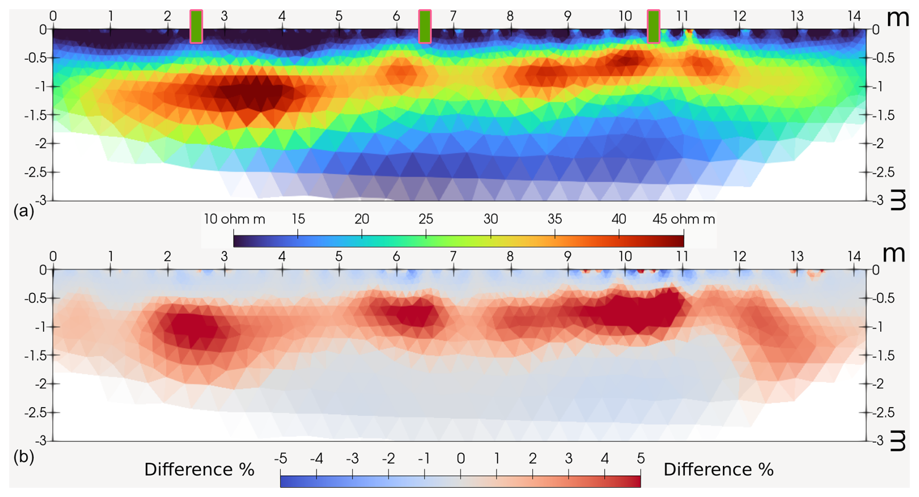
Figure 6 (a) ERT resistivity section acquired at 12:00 LT and (b) percentage difference between the first and last sections, acquired at 11:00 and 13:00 LT, respectively. The resistivity section highlights a resistive layer between 0.5 and 1.5 m depth, which is associated with the RWU. The more conductive layer above, where RWU is also expected, remains wet and more conductive because of the drip irrigation, which stopped at 11:00 LT, and possibly the effect of canopy cover together with the likely presence of active roots not in the deeper soil regions. The time-lapse percentage difference shows how the resistive regions become more resistive over time, which supports the RWU interpretation. In particular, the difference section highlights three regions around 2.5, 6.5, and 10.5 m whose spacings and positions correspond to the tree locations (green rectangles).

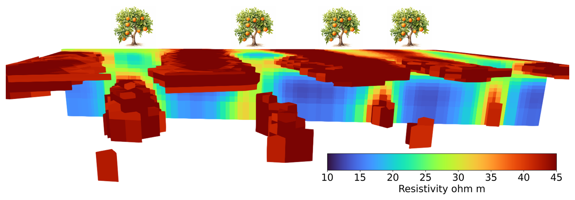
Figure 7 The 3D resistivity model obtained from the FDEM inversion, with a view perpendicular to the tree row direction. Within the model, the four tree rows are associated with low resistivity at the surface (irrigation lines) and higher resistivity below (RWU). Vice versa, the five interrows are associated with high resistivity at the surface (caused by direct evaporation with no tree canopy shadowing and absence of irrigation) and lower resistivity below (region less affected by direct evaporation and absence of tree roots, where the water content tends to persist as relatively high). A diagonal water movement from the irrigation line to the deeper interrow regions is supported by the fact that the shallow and deeper resistive regions are separated. The trees sketched in the image indicate the known position of the tree rows.

The spatial variability captured by the FDEM and ERT motivated the merging of the FDEM datasets through a kriging interpolation and their successive inversion. The optimized kriging for the ρ_a interpolation had a Gaussian variogram with a sill of 40 Ω²m², a range of 3.5 m, and a nugget equal to 2 Ω²m². The kriging anisotropy angle matched the azimuth of the tree rows, measured in QGIS. The merged dataset included the four GEM-2 datasets measured (as the two lowest frequencies were not used) and the six CMD-Explorer datasets (three coil separations with both coil orientations). The dataset was then inverted with EMagPy with the described parameters and model layers. The inversion converged at a root mean square percentage error of 11 % and returned the 3D model of resistivity shown in Fig. 7. The figure shows a transversal view of the inverted model, but it also extracts all of the values above 40 Ωm to highlight the alignment of the resistive regions along the tree rows and interrows. The inverted model is consistent with the above description of the individual datasets: the resistivity increases downward along the tree irrigation rows and upward along the interrows. A generally more conductive quarter-row divides the two, in line with the high-resolution surveys (Fig. 3). The inversion highlights the contrast between resistive and conductive regions, with resistivity values diverging toward 45 and 10 Ωm, respectively. The FDEM resistivity trend from the shallow irrigated layer (∼15 Ωm) to the deeper and drier RWU regions not yet reached by the water infiltration (∼45 Ωm) agrees with the ERT inverted section shown in Fig. 6. Small ERT vs. FDEM differences are observed and expected due to the vertical water redistribution between the ERT measurements and successive high-resolution FDEM surveys but also because of the higher resolution of the ERT surveys with 20 cm spacing relative to the FDEM and consequent different model discretization and inversion smoothing.

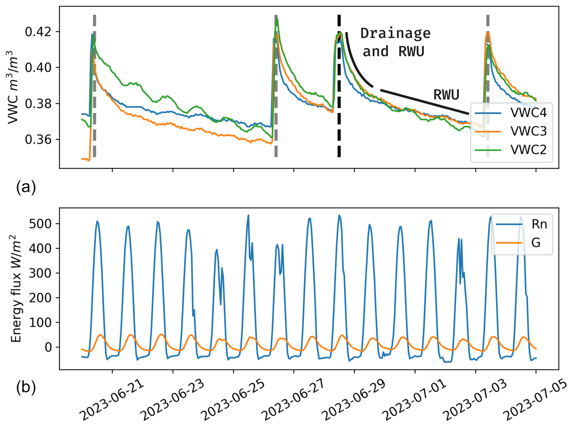
Figure 8 Time series of soil VWC (a) and measured energy fluxes (b) in the period of the field campaign (dashed line on 28 June). The VWC time series respond to the irrigation inputs reaching values around 0.42. From its maximum values, the VWC water first quickly drains subject to drainage and RWU. The VWC decrease rate slows and stabilizes when reaching the FC. The dashed gray lines indicate the other irrigations.

The laboratory water retention measurements that were performed on the eight soil samples yielded a VWC of 0.4 at field capacity (FC, −0.3 kPa) and of 0.28 at wilting point (WP, −15 kPa). These results indicate a significant water retention capacity and the possible presence of clay and organic matter. The standard deviations were 0.015 kPa at FC and 0.012 kPa at WP, which suggests relatively homogeneous soil characteristics. In line with the sample results, the gamma-ray survey did not identify significant spatial variability. Therefore, the results are expressed as average values and the associated standard deviation. The measured K percentage is estimated to be 0.6±0.1 %, while Th is estimated to be 3.7±0.7 ppm, and U is estimated to be 1.8±0.4 ppm. The total dose rate is equal to 4.7±2 nGy h⁻¹. These values agree with the retention curves obtained from the soil samples and the measured low electrical resistivities in the presence of clay mineral and organic matter (Omoniyi et al., 2013; Dierke and Werban, 2013).

The soil sensors recorded VWC changes during the 2023 growing season, including the period of the field campaign. However, the soil sensor in the northwest did not function correctly and was not considered. Figure 8a shows the recorded VWC time series from 21 June to 5 July. The VWC increases following the irrigations to values around 0.42, slightly above the FC measured in the soil samples. In fact, VWC initially drains more sharply, suggesting a combination of gravitational drainage and RWU. The VWC decrease rate slows and stabilizes when reaching FC. Figure 8b shows the measured net radiation (Rn) and soil heat flux (G). Both energy fluxes are relatively stable in the selected period, with net radiation maxima around 500 W m⁻² and soil heat flux maxima around 50 W m⁻².

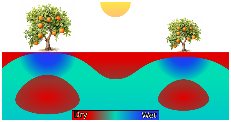
Figure 9 Conceptual model of spatial variability of volumetric water content (VWC) induced by irrigation and ET dynamics. In red are the drier and more resistive regions. The trees indicate the tree lines, where the shallow irrigation and deep RWU induce a wet-to-dry VWC profile along the tree lines. On the contrary, shallow evaporation and deep water redistribution lead to a dry-to-wet VWC profile along the interrow. At the transition depth, the quarter-row is wetter, with dryer soil on both sides.

The above results agree with a conceptual model that distinguishes tree rows, interrows, and quarter-rows (Fig. 9). The specific spatial variability of electrical resistivity suggests that VWC is the dominant factor. This agrees with the homogeneity of the soil samples and gamma results. Shallow irrigation and deep RWU induce a wet-to-dry VWC profile along the tree lines. Shallow evaporation and deep water redistribution lead to a dry-to-wet VWC profile along the interrow. At the transition depth, the quarter-row is wetter (more conductive region) with dryer soil on both sides. The soil sensors indicate a relatively short interval in which water (above the FC) drains toward the deeper and drier region and the interrows.

4 Hydrological model

The conceptual model was used to implement a 3D (CATHY) numerical model that includes both soil water dynamics (RWU and irrigation) and ET. The model was discretized and constrained as described, i.e., coupling geophysical spatial information and VWC time series, and using the known forcing and water inputs as boundary conditions. Figure 10 shows the CATHY-simulated VWC distribution at the time of the FDEM measurements and the fitting of the VWC time series from the co-located soil sensors (20 cm depth along the tree rows, Figs. 1 and 2). The figure shows a good spatiotemporal agreement of the simulated VWC distribution with field observations. In Fig. 10b, the simulated VWC values follow adequately the measured VWC time series. The simulation reproduces (1) the three sharp increases associated with the irrigations, (2) the quick VWC drop occurring right after the irrigation, and (3) the stabilization of the VWC change with time. The fitting remains good over the explored period of 14 d, indicating the model stability with respect to the irrigations and successive ET dynamics. Spatially, the simulation reproduces the key aspects present in the conceptual model derived from the FDEM data and relevant inverted model (Fig. 7). Tree rows and interrows are well distinguished by their opposite VWC profiles, with the widths and depths of the VWC transition reflecting the FDEM model. The model also reproduces the presence of a transition region (quarter-row) that connects the irrigation bulb with the deep part of the interrow, also relatively wet because of the reduced impact of the evaporation at depth. The adopted Mualem–van Genuchten parameters had an air entry head of 1 m, a residual VWC of 0.08, a saturation VWC of 0.48, and n equal to 1.25. These values reproduce the VWC values measured in the laboratory at FC (0.4) and WP (0.28) and agree with the presence of clay and organic matter (Carsel and Parrish, 1988). Costa et al. (2013) reported similar VWC values (0.41 and 0.31) for a sandy clay loam in a shallow soil horizon with 4 % organic matter (their Tables 1 and 2). Rab et al. (2011) reported values of 0.43 and 0.28 for a silty clay loam, with an average organic matter of 1.2 % (their Table 5). The van Genuchten parameters also agree with the transition from the drainage slope to the extraction RWU slope observed in the VWC time series after irrigations (Wilcox, 1962; Dittmar et al., 2021).

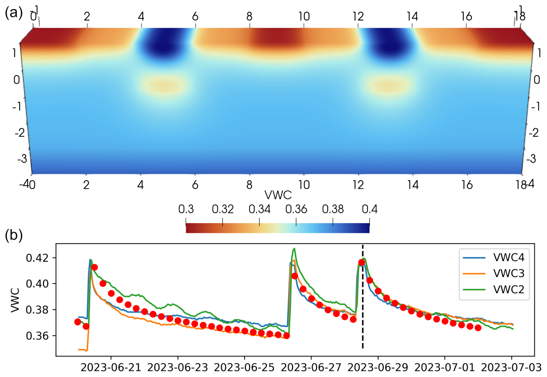
Figure 10 CATHY hydrological simulation of the spatial distribution of the VWC at the time of the field campaign (a) and its temporal variability over a period of 14 d. The spatial distribution reproduces the conceptual model derived from the FDEM and ERT results. In (b) is the simulated VWC (red dots) extracted from the model position that matches the three soil moisture sensors in the field (VWC2–4, 20 cm depth along tree lines, Figs. 1 and 2). The time series show the model-consistent response, reproducing three irrigation periods and successive ET responses.

The hydraulic conductivity estimated from the CATHY calibration is $\mathrm{1}\times {\mathrm{10}}^{-\mathrm{5}}$ m s⁻¹. Although different values of hydraulic conductivity were tested, the spatiotemporal information strongly constrained its value. Larger values would lead to a steeper drop drainage of the VWC after the irrigation and to an excessively large wet and/or conductive irrigation bulb along the tree rows. The hydrological simulations also explored the possible anisotropy of the hydraulic conductivity, with values that were larger in the horizontal direction (Fan and Miguez-Macho, 2011), as reported for natural and managed soils (Pirastru et al., 2017; Brooks et al., 2004; Shaw et al., 2001; Bagarello et al., 2009). However, introducing this anisotropy excessively widened the irrigation bulb, led to a shallower RWU dry region, and shifted the break-point in the time series. Therefore, an isotropic hydraulic conductivity has been hypothesized, with the interpretation that the tree roots could channel the water and balance the possible intrinsic anisotropy of the soil hydraulic conductivity. This also explains the relatively large value of the hydraulic conductivity despite the presence of clay and organic matter (Carsel and Parrish, 1988; Schaap et al., 2001).

The potential ET was maintained as homogeneous for all simulated days, reflecting the stable sunny conditions (Fig. 8) and considering a maximum value of 7 mm d⁻¹ based on the available eddy covariance data (located within the farm property 500 m from the site). This value agrees with the previous studies conducted in the area (Vanella et al., 2025; Mary et al., 2019) and other studies conducted under similar Mediterranean conditions (Cammalleri et al., 2013; Autovino et al., 2016, 2018; Abedi-Koupai et al., 2022). Considering the geometry of the tree rows (partial tree coverage) and the limited ET from the dry interrows, these values are also consistent with the resulting values of ET from irrigated orange trees. For example, Mishra et al. (2021) reported transpiration values from 2 L d⁻¹ in 5-year-old trees to 5 L d⁻¹ in 15-year-old trees. Mira-García et al. (2021) reported actual RWU values ranging between 2 and 3 L d⁻¹ for young lime trees under Mediterranean summer conditions. Hou et al. (2023) reported values between 2 and 3 mm d⁻¹ in orange trees under similar conditions of air temperature and net radiation. The CATHY simulation showed that the ET value controls the slope of the VWC time series after the initial drainage period, i.e., the tail after the break-point. The simulated slope agrees with the values measured by the co-located soil sensor (Fig. 10b). The ET also controls the size of the RWU dry region, while its depth mostly depends on the hydraulic conductivity. For example, the dry RWU region would become enlarged and overlap the interrow dry region when the ET value was too large, e.g., maintaining the 7 mm d⁻¹ ET rate for the entire day.

5 Discussion

This agrogeophysical study explores the potential and challenges in high-resolution FDEM mapping, aiming to develop a more quantitative coupling with soil and atmospheric sensors through a hydrological model that includes the spatiotemporal dynamics of irrigation and RWU–ET. On the one hand, the results show how FDEM can address the common lack of spatial information expected to inform present and future precision agriculture practices. The 1 d characterization successfully led to a conceptual model that highlights the interplay of irrigation and RWU along the tree rows, including the widths and depths of the affected regions (Fig. 9). The characterization also captured the opposite VWC profiles along the interrows and the details of the transition region, i.e., the interaction between tree rows and interrows. The irrigation bulbs spread toward the interrows and connect to their deeper and wetter regions, dividing the shallow-transpiration and deeper-RWU regions. Thanks to the convenience of the FDEM surveying practice, local variability within this general model was resolved over the entire field, both laterally and vertically (Fig. 7). The RWU–irrigation dynamics are central to precision agriculture and irrigation strategies. Nonetheless, the interrow hydrology and its coupling with the plant rows has been receiving significant attention because of its impact on vegetation, soil quality and erosion, and general ecosystem resilience (Bagagiolo et al., 2018; Morlat and Jacquet, 1993). The 3D FDEM characterization was successfully coupled with the soil sensors, soil samples, and ERT sections thanks to its large spatial extension, sufficient spatial resolution, investigation depth, and coverage of both tree rows and interrows. While FDEM has long been recognized as an ideal and promising solution in agrogeophysics (Garré et al., 2021; Boaga, 2017; O'Leary et al., 2024; Von Hebel et al., 2021), this study first realizes such expectations in an orchard, whose 3D subsurface variability is a complex combination of RWU, irrigation, ET, and row–interrow dynamics.

On the other hand, this study also highlights critical methodological challenges that are commonly hidden behind seemingly simple survey choices and processing steps, potentially limiting the otherwise wide potential of FDEM in agrogeophysics. A Geophex GEM-2 and a CMD Mini-Explorer were used, with the latter in a vertical and horizontal configuration. Initial GEM-2 measurements were also performed at 1 m height above the ground, but the results and the modeling of the sensitivity profiles motivated ground-level measurements (Fig. 4), which captured the deeper-RWU region (Figs. 1 and 3). The choice of instruments and survey design was suitable for this study, but this was not obvious a priori, nor is a similar combination always possible or adopted. It is highlighted how the use of a single instrument would miss or misinterpret either the RWU or the ET. While two intermediate-depth datasets captured both aspects (Fig. 5), the required combination with higher-resolution surveying, sensitivity analysis, and processing, and visualization was only possible as an a posteriori effort, after the conceptual model was derived. In turn, these datasets and their detailed analysis were essential to confirm the vertical connection between the two instruments and to finalize the conceptual model, defining the actual extent and transition of the conceptualized regions (Fig. 9).

The individual FDEM datasets may also differ because of their instrumental drift or calibration (Blanchy et al., 2024; Boaga, 2017; McLachlan et al., 2021; Delefortrie et al., 2014). In this study, the two lowest frequencies of the GEM-2 measured apparent conductivities that were anomalously low. This fact initially motivated an ERT-based calibration of the FDEM data in EMagPy, but the two datasets were eventually discarded because they also had a low signal-to-noise ratio level. Nonetheless, the presence of anomalous datasets would have been hard to detect in the absence of the ERT section and sensitivity analysis, which highlighted how the low conductivities were inconsistent with the other FDEM datasets and the ERT results.

The quantitative use of the two instruments required spatial alignment and joint inversion. The standard GPS systems did not provide a reliable alignment of the surveys relative to the spatial scale of the orchard and the associated need for a fine spatial resolution. While the corrections of the off-centering and random errors were successful, they required time-consuming GIS corrections for both intra- and inter-dataset shifts and alignments. The GPS marker positions collected during the survey and the simple geometry of the site surely helped in this context. In particular, the off-centering corrections were motivated by the typical sinusoidal distortion (Choi and Kim, 2020) of the straight tree rows. The off-centering correction required the implementation of a specific and automatic procedure because of its complexity and the numerousness of the FDEM datasets. Yet, weaker ρ_a contrasts or a more variable tree distribution would have hindered this correction and, thus, the alignment with the Mini-Explorer. In general, it should be stressed that, in order to make suitable use of FDEM data for this type of application, precise attention to high-resolution positioning will have to be ensured. Otherwise, most of the most important spatial variability features can be overlooked.

After the GPS alignment, the surveys were interpolated over a common grid to allow the joint inversion. Because of the spatial heterogeneity and anisotropy in the general orchard geometry, the interpolation required careful parameterization of the kriging algorithm (Fig. 5). Other interpolation algorithms could not preserve the spatial features present in the datasets, particularly because of the transversal smoothing between tree rows and interrows. Again, this aspect becomes essential when the ρ_a contrasts are weak (e.g., secondary resistive features in Fig. 5), even more so if the anomalies are relatively narrow or poorly sampled (Fig. 1a). The interpolation step is also tightly coupled with the survey direction and smoothing of the data. The smoothing is commonly applied to the FDEM data to address the variability caused by the noise or survey instability (McLachlan et al., 2021). While automation is critical for adoption, the frequent use of simple smoothing solutions (i.e., moving average) is in contrast with the spatial variability and anisotropy of many agricultural sites. For example, the resistive anomaly captured by the transversal GEM-2 larger-scale survey would have been strongly altered by a 1D moving average because of the survey direction and narrow target anomaly (Fig. 1a).

Addressing the above challenges in a very careful manner allowed for an effective coupling of the geophysical results with data from the soil and atmospheric sensors. In particular, the final 3D FDEM model successfully added the spatial dimensionality into the VWC time series measured by the commonly deployed soil sensors (Yu et al., 2021; Garré et al., 2021). This led to a conceptual model that, in turn, guided the implementation of a CATHY-based hydrological model (Figs. 9 and 10). In this respect, the CATHY hydrological model allows the integration of all available data (spatially extensive geophysical data and time-intensive single-probe time series) in order to construct a fully consistent conceptual model of the shallow subsurface; in this study, the model expresses the complementarity of specifically timed FDEM characterizations and long-term time series. The CATHY hydrological model reproduces the observed spatiotemporal dynamics with parameters that agree with soil laboratory analysis, gamma-ray surveys, and reviewed literature. Specifically, the soil hydraulic properties (Mualem–van Genuchten parameters and hydraulic conductivity) were constrained to specific values that reproduced the field's spatial and temporal variabilities in terms of the VWC (Fig. 10). This is a significant result considering the fact that hydraulic properties and VWC ultimately control the presence and mobility of water, nutrients, and pesticides (Vereecken et al., 2007, 2008; Bünemann et al., 2006; Patzold et al., 2008). The ET was better known from a literature review of comparable studies and eddy covariance estimates. Hence, the ET was set as a known forcing, which limited the number of free parameters and realistically tested the stability of the model during a period of 14 d and three irrigations (Fig. 10). While this study did not explore data assimilation approaches and uncertainty analysis, the hydrological parameters appeared to be well constrained by the available combination of spatial and temporal information. As discussed above and in the specific section, changing the soil hydraulic properties significantly impacted both the extension and the depth of the conceptualized regions, as well as the misfit relative to the measured VWC time series. This suggests that future works could positively explore advanced quantitative investigations of the hydrological model. Data assimilation approaches may also ease the integration of successive FDEM surveys, whose design and timing may be guided by the hydrological model to target specific aspects of the growing season.

Our FDEM results showed a number of important effects related to the instrument footprints, for example, at the turns of the high-resolution Mini-Explorer surveys (Fig. 3) and the differences between the longitudinal and transversal GEM-2 results (Fig. 1). The footprint effects become significant because of the anisotropy and spatial scale of the orchard relative to the desired high resolution (Klose et al., 2022). In this respect, this study points toward the development of 2D and/or 3D FDEM inversion codes (Klose et al., 2022; Heagy et al., 2017; Guillemoteau and Tronicke, 2016) and a better understanding of the FDEM instrument footprints (Guillemoteau and Tronicke, 2015). This development would also need to account for the relative positions of the instrument coils and, thus, the surveying direction, for example, with the proposed algorithm for the correction of the GPS off-centering. In contrast to other FDEM applications, this is especially relevant in agrogeophysics because of the subtle conductivity contrasts, typically dominated by the VWC, and the need for a very fine (sub-meter) spatial resolution. Nonetheless, this study also showed how surveying in multiple directions and with different spacings can mitigate the impact of the footprint effects, improving the interpretation and interpolation of the results and, thus, the final 3D FDEM model (Figs. 5 and 7).

Time-lapse geophysical measurements are central to hydrogeophysics (Rubin and Hubbard, 2005; Binley et al., 2015). However, the trade-off between time-lapse measurements and spatial characterization remains because of intrinsic time and economical resource limitations and method characteristics (e.g., ERT and FDEM or others). This study adopted a variant hydrogeophysics approach where the FDEM mapping has been coupled with temporal information from soil and atmospheric sensors, which are commonly available and more conveniently provide temporal information. This perspective aligns with the concept of agrogeophysics as agricultural sites are being increasingly instrumented, and supporting information is often available (McBratney et al., 2005; Karunathilake et al., 2023). The surface–subsurface hydrological model appeared to be necessary to fully explore and take advantage of such coupling involving very different datasets, both aboveground and belowground. This added complexity, however, connects with existing practices and methods, such as eddy covariance, soil sensors, and cosmic-ray neutron sensing, as well as with the need for a better understanding and prediction capability in precision agriculture and irrigation management (Beven, 2008; Javansalehi and Shourian, 2024; Xi et al., 2017).

Overall, this study presents an agrogeophysical FDEM application that focuses on small-scale aspects that had not been properly considered in previous studies. The presented challenges explain the lack of similar studies and should be considered when discussing the FDEM convenience and adoption. The successful characterization and its hydrological coupling with soil and atmospheric sensors motivates such future efforts in the field of agrogeophysics.

6 Conclusions

This agrogeophysical study explored the potential and challenges in high-resolution FDEM mapping, aiming at a quantitative coupling of extensive hydrogeophysical data with soil and atmospheric sensors through a 3D hydrological model that reproduces the spatiotemporal dynamics of irrigation and RWU–ET. Several FDEM datasets and ERT time-lapse measurements were collected. Additional supporting information was also available from soil and atmospheric sensors, which are becoming increasingly common at agricultural sites. The first goal, relating to the FDEM methodological challenges, motivated a careful investigation of the survey choices and processing steps. Several challenges and pitfalls were recognized and addressed to obtain a final 3D inverted model of soil resistivity, starting from the choice of a suitable combination of instruments and survey configurations, directions, and spatial resolutions. An initial exploratory phase with survey variations was essential, but the success of the characterization was only confirmed after time-consuming processing, visualization, and interpretation steps. These steps included GPS positioning corrections, data filtering, kriging interpolation, and sensitivity analysis. Addressing the above challenges allowed the coupling of the FDEM characterization with soil and atmospheric sensors. This led to a conceptual model that guided the implementation of a 3D surface–subsurface hydrological model. The hydrological model was necessary to fully take advantage of such coupling involving very different datasets and, thus, connect the aboveground and belowground processes. This approach has the great advantage of making full use of existing practices and methods, such as eddy covariance, soil sensors, and cosmic-ray neutron sensing, adding the information coming from spatially dense (and time-lapse) non-invasive data that are the fundamental building blocks for the construction of a successful, scientifically sound, site conceptual model. Beyond the integration of available datasets, such conceptual and numerical models align with the need for a better understanding of and prediction capability in precision agriculture and irrigation management.

Appendix A: Abbreviations

ET	Evapotranspiration
VWC	Volumetric water content
RWU	Root water uptake
FC	Field capacity
WP	Wilting point
ρa	Measured apparent electrical resistivity
ρ	Electrical resistivity
ERT	Electrical resistivity tomography
FDEM	Frequency-domain electromagnetics