Terrain is a stronger predictor of peat depth than airborne radiometrics in Norwegian landscapes

Peatlands are Earth's most carbon-dense terrestrial ecosystems and their carbon density varies with the depth of the peat layer. Accurate mapping of peat depth is crucial for carbon accounting and land management, yet existing maps lack the resolution and accuracy needed for these applications. This study evaluates whether digital soil mapping using remotely sensed data can improve existing maps of peat depth in western and southeastern Norway. Specifically, we assessed the predictive value of lidar-derived terrain variables and airborne radiometric data across two, >10 km² sites. We measured peat depth by probing and ground-penetrating radar at 372 and 1878 locations at the two sites, respectively. Then we trained Random Forest models using radiometric and terrain variables, plus the national map of peat depth, to predict peat depth at 10 m resolution. The two best models achieved mean absolute errors of 60 and 56 cm, explaining one-third of the variation in peat depth. Terrain variables were better predictors than radiometric variables, with elevation and valley bottom flatness showing the strongest relationships to depth. Radiometric variables showed inconsistent and weak predictive value – improving performance at one site while degrading it at the other. Our remote sensing models had better accuracy than the national map of peat depth, even when we calibrated the national map to the same depth data. Still, weak relationships with remotely sensed variables made peat depth hard to predict overall. Based on these findings, we conclude that digital soil mapping can improve the existing, national map of peat depth in Norway, but detailed local maps are best made from tailored field measurements. Together, these pathways promise more accurate landscape-scale carbon stock assessments and better-informed land management policies.

1 Introduction

Peat soils are a terrestrial carbon stock of global importance. They store 450–650 Gt of carbon, or about 30 % of global soil carbon, despite covering only 2 %–3 % of Earth's land (Xu et al., 2018; Friedlingstein et al., 2020; UNEP, 2022). Peatlands (areas with peat soil) are more carbon dense per square meter than any other ecosystem (Temmink et al., 2022). This makes them crucial to climate change mitigation. Intact peatlands sequester carbon and overall produce a negative temperature forcing (Joosten et al., 2016). When disturbed – often by conversion to another land use – they can produce large greenhouse gas emissions (Ma et al., 2022).

One of the keys to the areal density of peatland carbon stocks (and variation therein) lies in the third dimension: their depth. Peat soils range from zero to over ten meters deep (Widyastuti et al., 2024). Their depth depends on the rate and duration of organic matter accumulation, potentially over thousands of years (Loisel et al., 2014; Joosten et al., 2016). In the anoxic and acidic conditions created by a high water table, plant material decay is slightly outweighed by new growth, and the surplus carbon is laid down as peat.

Peatlands are most common at high latitudes, and in regions with high cover they are frequently converted to human land use (UNEP, 2022). They are attractive for agriculture and forestry because they are flat, treeless, and have developed soils, but other land uses also displace peatlands. In Norway – where flat lowland is relatively scarce but upward of 9 % of the land area is peatland (Bryn et al., 2018; Bakkestuen et al., 2023) – lawmakers have restricted peatland afforestation and cultivation in recent decades. Since then, a larger proportion of peatland loss is driven by construction (Flaget et al., 2024).

Variation in peat depth and its spatial distribution is often overlooked in land use planning and carbon accounting because peat depth is not mapped with sufficient coverage, resolution, or accuracy (Beilman et al., 2008; Hastie et al., 2022; UNEP, 2022). Maps are crucial because, unlike spatially aggregated estimates, they link high-level targets to specific management decisions (OECD, 2022). Maps of peat depth also make it possible to quantify the effect of specific management decisions and thereby understand how local outcomes contribute to regional and national outcomes (OECD, 2022).

Measuring peat depth on the ground is straightforward, and a field survey can map a small area at low cost. However, surveying large areas is impractical when depth varies widely over short distances (e.g., 10 m) – as in many peatlands (Torppa, 2011; Proulx-McInnis et al., 2013; Henrion et al., 2024). A complementary approach from soil science is digital soil mapping (DSM). DSM scales up field measurements from a set of locations to a wider area, by relating the measured values to other variables mapped over the area of interest, through a statistical model. This approach has grown in importance with the availability of remotely sensed data and the advancement of machine learning methods (Minasny et al., 2019; Wadoux et al., 2020).

The crux for DSM of peat depth is the relationship between peat depth and the other, mapped predictors. For DSM to be effective, these relationships must be strong and consistent over the area of interest. They can be purely correlative rather than causal, but mechanistic relationships are stronger and more consistent than non-causal ones. The scorpan framework for DSM suggests seven predictor classes to explore: other soil properties, climate, organisms, relief (topography), parent material, age, and spatial position (McBratney et al., 2003).

For peat depth, the most practical and widespread scorpan factors are relief and spatial position. Spatial position is unique because it is always known (with varying accuracy). However, the short range of spatial autocorrelation in peat depth limits its mapping value (Hengl et al., 2004). Relief, or topography, is widely and accurately mapped in digital terrain models (DTMs). For example, most of mainland Norway has at least one elevation measurement per square meter from airborne light detection and ranging (lidar) surveys. Moreover, mechanisms of peat formation are linked to topography.

Studies have consistently shown relationships between peat depth and topography, though the specific patterns vary. One of the most robust relationships is a negative correlation between depth and terrain slope (e.g., Holden and Connolly, 2011; Parry et al., 2012; Gatis et al., 2019). Peat depth also changes with elevation in many contexts, but with inconsistent directionality (e.g., Holden and Connolly, 2011; Parry et al., 2012; Rudiyanto et al., 2016, 2018; Koganti et al., 2023; Li et al., 2024). Also more complex derivations of topography, such as the Topographic Wetness Index and the Multi-Resolution Valley Bottom Flatness index, have shown associations with peat depth (e.g., Rudiyanto et al., 2018; Koganti et al., 2023; Li et al., 2024; Pohjankukka et al., 2025). Some of the variation between studies in quantifying these relationships is undoubtedly attributable to issues of spatial scale – both the scaling of the topographic predictors and the resolution of the peat depth analysis.

Another set of predictors related to peat depth are measurements of natural radioactivity from the ground surface. Gamma-ray spectrometry can survey the activity (decay counts per second) from radioactive isotopes in bedrock and mineral soils: potassium-40, uranium-238, and thorium-232 (Beamish, 2014; Reinhardt and Herrmann, 2019). Although survey measurements are commonly reported as ground concentrations (linearly scaled from decay counts per second), in peatland environments these predictors do not reflect the concentration of radionuclides near the ground surface, but rather the radiation intensity after attenuation by the peat overburden. Deep soil with high water content will attenuate radiation most (Beamish, 2013; Reinhardt and Herrmann, 2019). Thus, reported ground concentrations can be statistically informative about peat soils, even if not physically correct, with respect to two scorpan factors: other soil properties and parent material (McBratney et al., 2003).

Although theory suggests that one meter of peat may fully attenuate radiometric signal (Beamish, 2013; Reinhardt and Herrmann, 2019), empirical investigations show that the association between peat depth and radioactivity can extend beyond the first meter (Keaney et al., 2013; Gatis et al., 2019; Koganti et al., 2023). Radiometric data are increasingly available over large areas (Minasny et al., 2019; Baranwal and Rønning, 2020), and – insofar as they are predictive of peat depth – this presents an opportunity for DSM.

The effectiveness of DSM depends not only on the methods and data, but also on the characteristics of the mapping area. Norway may be instructive in this respect because its peatlands vary widely across climates and topographies. Norway has 22 peatland mesotopes, with different hydrology, formation, and development – from topogeneous or soligeneous fens to blanket or raised bogs (Joosten and Clarke, 2002; Lyngstad et al., 2023). These mesotopes have fundamentally different geomorphology, which suggests that relationships between peat depth and terrain or radiometric predictors may vary by landscape.

The only systematic mapping of peat depth at the national scale in Norway comes from surveys meant to identify arable land. After scattered efforts in the early 20th century, a comprehensive round of surveying was completed 1964–2001 as part of a wider land cover mapping in Norway (Bjørdal, 2007). This survey produced the initial maps from which Norway's most detailed updated land cover datasets are derived – including the AR5 and DMK datasets used in this study and described later. Because of its agricultural and silvicultural focus, the survey covered only productive areas below the tree line, and peat depth was measured only in places judged to be potentially arable or afforestable (Ahlstrøm et al., 2019). Field surveyors carried a 1 m probe and they measured peat depth as a categorical variable: shallow (<1 m), or deep (>1 m). These classes were assigned to whole polygons, so spatial resolution is on the order of hectares. The number of measurements per unit area was not standardized but probably low.

The push for nature-based climate solutions motivates for extensive mapping of peat depth, to identify peatlands with rich carbon stocks to avoid their conversion and prioritize their preservation or restoration (Strack et al., 2022). Although ground surveys of peat depth are accurate and feasible across small areas, having landscape-scale maps available before detailed investigation increases the option space for spatial planning and land management. For example, the Norwegian Public Roads Administration routinely measures peat depth during geotechnical work before road construction, but by that time, the route of the road is already set. With a landscape-scale peat depth map, planners could better compare the climate impact of different routes. To make landscape-scale maps possible, more studies need to investigate the relationships between peat depth and topographic or radiometric variables, to determine how strong and consistent these are.

Here, we assess how well remotely sensed topographic and radiometric data can predict peat depth at two contrasting sites, with a view toward revising regional and national maps in Norway. Specifically, we aim to: (1) quantify the accuracy of predictions from topographic and radiometric variables, and (2) identify key predictive variables. Reflecting on our results and the need for continued improvement in peat depth maps, we close by discussing implications for digital soil mapping of peat depth.

To our knowledge, this is the first study to predict continuous peat depth from airborne radiometric data using machine learning. Where airborne radiometric data have previously been used to predict continuous peat depth, it has been through modeling techniques less suited for prediction and spatial extrapolation (e.g., Keaney et al., 2013; Gatis et al., 2019; Siemon et al., 2020). Where machine learning has previously been used with airborne radiometric data, it has been to predict peat extent or depth classes rather than continuous depth (e.g., O'Leary et al., 2022; Pohjankukka et al., 2025).

2 Materials and methods

2.1 Sites

To assess the predictive value of terrain and radiometric data for mapping peat depth, we chose two sites with conspicuously different physical geography: Skrimfjella in eastern Norway (Fig. 1a) and Ørskogfjellet in western Norway (Fig. 1b). These sites were chosen because they were covered by radiometric data from airborne surveys, had relatively little built-up area, and were accessible by road. Ørskogfjellet was additionally chosen for its relatively uniform bedrock geology, which should improve the peat depth signal in radiometric data, all else being equal (Minasny et al., 2019).

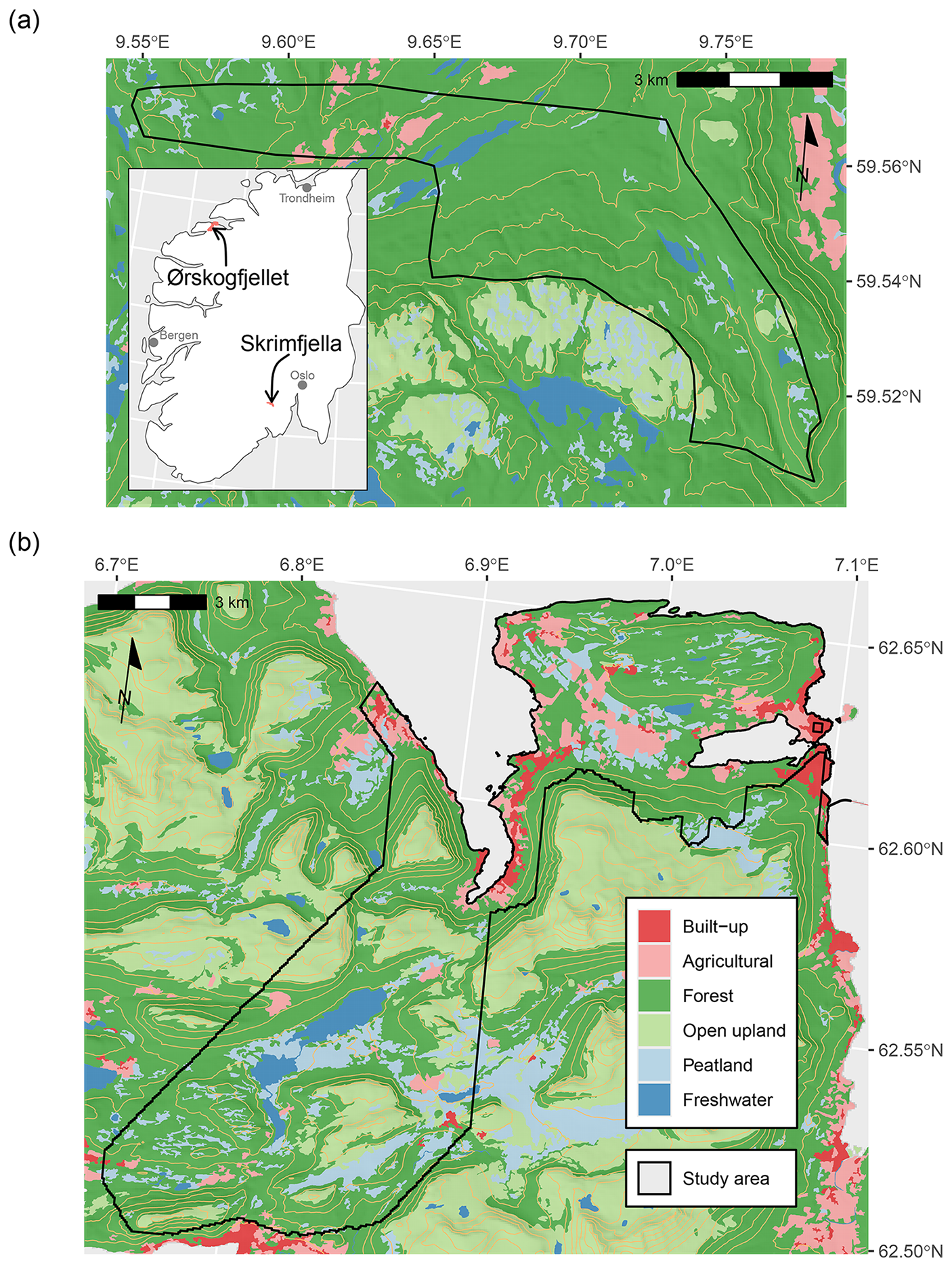
Figure 1 Study areas with land cover at Skrimfjella (a) and Ørskogfjellet (b). To fit the scale of the maps, the land cover shown here is from the AR50 national land resource dataset, which has simplified geometry with respect to the AR5 dataset that is used in the study. Terrain is visualized with light orange contour lines at intervals of 100 m, and a hillshade with slope 45° and azimuth 225°. AR50 data are from Norwegian Institute of Bioeconomy Research under the Norwegian Licence for Open Government Data (https://data.norge.no/nlod/en/1.0, last access: 19 September 2024) and terrain data are from the Norwegian Mapping Authority under the Creative Commons Attribution 4.0 International license (https://creativecommons.org/licenses/by/4.0/, last access: 20 September 2024) © Kartverket.

At Skrimfjella we delineated a study area of 34 km² based on radiometric coverage (limiting to the west) and accessibility (limiting to the south), as part of a pilot project (Fig. 1a). In Norway's AR5 national land cover dataset (“areal resources in scale 1:5000”; Ahlstrøm et al., 2019), 1.5 km² (4.5 %) of the study area is classified as “mire” – defined as areas with mire vegetation and at least 30 cm of peat depth. Relatively sparse peatland cover did not disqualify the area for our purposes, since we were also interested in peatland extent mapping in the pilot project. The study area has a diverse bedrock, with 32 % alkali feldspar granite, 26 % marlstone, 10 % granite, 8 % monzonite, 7 % sandstone, 6 % limestone, and five other rock types with 1 %–5 % coverage (Geological Survey of Norway, 1:250 000 dataset). It is almost without human infrastructure, dominated by conifer forest, and borders on a nature reserve. Its mean elevation is 438 m a.s.l. (range 223–711 m, IQR 351–509 m), and its mean slope at 10 m resolution is 10.8° (IQR 4.6–15.1°).

At Ørskogfjellet we defined a study area of 124 km² which basically followed the southernmost part of the radiometric survey extent (Fig. 1b). In the AR5 dataset, 15.3 km² (12.4 %) of the study area is classified as mire. Bedrock in the area is 84 % granitic gneiss, 11 % granite, and 5 % aluminium silicate gneiss (Geological Survey of Norway, 1:250 000 dataset). This study area is mostly forested, but also contains considerable farmland and open upland, and has several large lakes. Its mean elevation is 211 m a.s.l. (above sea level) (range 0–807 m, IQR 73–310 m), and its mean slope at 10 m resolution is 13.0° (IQR 4.7–18.3°).

2.2 Peat depth predictors

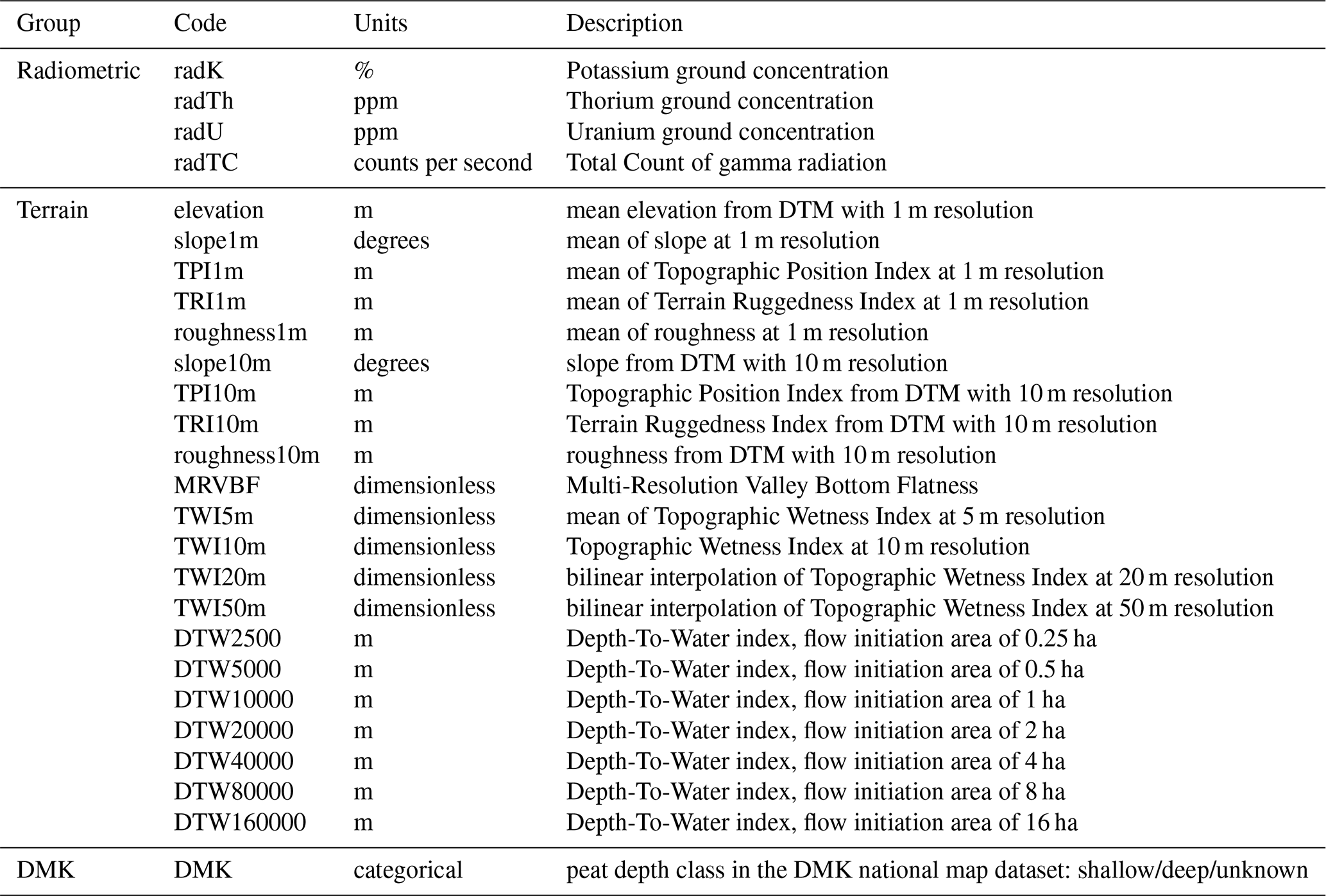
We created the same suite of peat depth predictors for both sites (25 continuous and 1 categorical; Table 1). All continuous predictors were derived either from an airborne radiometric survey or from a DTM. From the radiometric surveys, we simply used the four variables produced by the Geological Survey of Norway: ground concentration of potassium, thorium, uranium, as well as total count. From the DTMs we calculated several land surface parameters, ranging from simple terrain indices to more complex geomorphometric and hydrological variables (Maxwell and Shobe, 2022). The categorical predictor was peat depth class, from a national map dataset. Predictor preparation is described in more detail below.

Table 1 Twenty-six candidate predictors of peat depth. Note that each continuous predictor contributes one variable to the model while the single categorical predictor (DMK) contributes two binary variables, corresponding to its three levels (one level is used as the reference). This results in a total of 27 variables.

We chose a spatial resolution of 10 m for our predictors, depth sampling, and modeling. We considered this a reasonable compromise between DTM resolution (1 m) and small peatlands on the one hand, and airborne radiometric resolution (50 m) on the other hand.

2.2.1 Radiometric

The Geological Survey of Norway conducted and processed radiometric surveys over our study areas, as reported in Baranwal et al. (2013) and Ofstad (2015). They provided us for each site four variables at 50 m resolution, which we downscaled to 10 m resolution by cubic spline resampling. Sensitivity analysis showed that Pearson correlations between cubic spline and bilinear resampling methods exceeded 0.995 for all radiometric variables, so we are confident that the choice of resampling method did not affect our results.

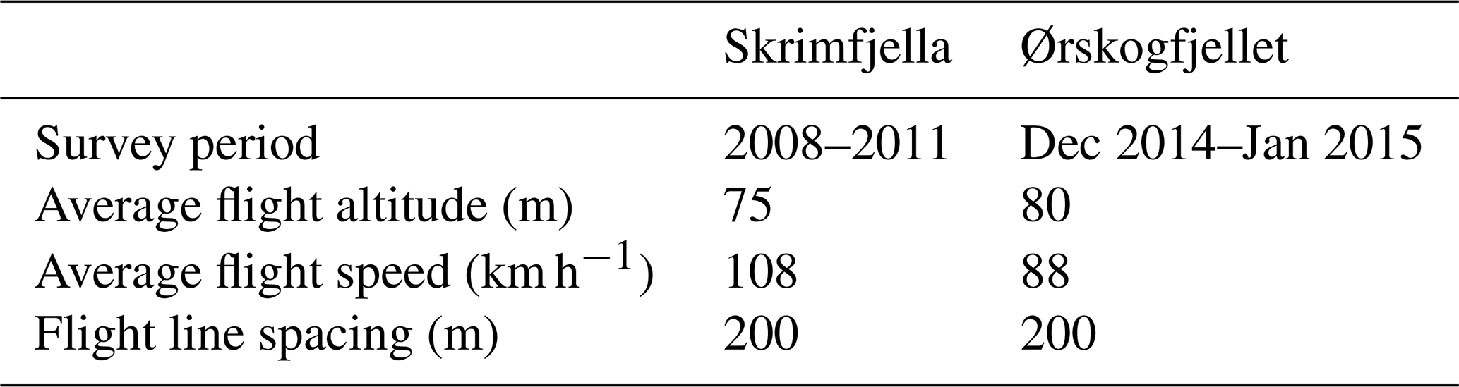
The radiometric surveys were conducted with 75–80 m average flight altitude, 88–108 km h⁻¹ average flight speed, and 200 m flight line spacing (Table A1). Spectrometer count rates were calibrated to known concentrations of potassium, thorium, and uranium in mobile pads. Data were processed following standard procedures outlined by the International Atomic Energy Association. Processing included: correction for aircraft and cosmic background radiation, correction for radon in the air, window stripping of the gamma ray spectrum, correction for flying height, conversion of count rates to ground concentrations, and finally gridding to 50 m resolution with micro-leveling. At Ørskogfjellet an additional convolution filter was added to smooth the gridded data.

Although radiometric data must be in units of counts per second to model attenuation directly (O'Leary et al., 2022), we used the radiometric data as provided to us: in units of concentration for potassium, thorium, and uranium (converted from counts per second by scalar calibration factors). The monotonic transformation between counts per second and concentration has no effect on the tree-based machine learning algorithm that we used to model peat depth (Hastie et al., 2009). We also used the total count variable as provided, rather than calculating a gamma dose rate based on the potassium, thorium, and uranium (as was done in Gatis et al., 2019), because these were highly correlated at both study sites (ρ=0.989, 0.986), and because conversions to dose rates are approximations (IAEA, 2003).

2.2.2 Terrain

For terrain-derived predictors, we obtained 1 m resolution rasters from the national DTM (https://creativecommons.org/licenses/by/4.0/, last access: 9 September 2024, CC BY 4.0, Norwegian Mapping Authority). The DTM for Skrimfjella was produced from airborne laser scanning surveys in 2015 and 2022, with laser point density of 5 pts m⁻². For Ørskogfjellet, the DTM was produced from a 2015 survey with 2 pts m⁻². Where necessary, DTMs were resampled to the coordinate reference system of the radiometric data.

We used the terra R package (v.1.8; Hijmans, 2025) to calculate from the DTMs: slope, Topographic Position Index (difference from mean of eight neighbors), Terrain Ruggedness Index (mean of absolute differences from eight neighbors), and roughness (range in the nine-cell neighborhood). These were derived at two scales to produce eight different predictors; we either calculated the indices at 1 m DTM resolution and then aggregated to 10 m resolution, or aggregated to 10 m DTM resolution and then calculated the indices. This kind of multiscale feature engineering of land surface parameters has been found to improve machine learning predictions of soil properties (Miller et al., 2015; Dornik et al., 2022; Newman et al., 2023). We know that peat depth tends to vary at fine scales in Norway, which is why we chose 1 and 10 m resolutions (Maxwell and Shobe, 2022). We also calculated the Multi-Resolution Valley Bottom Flatness index, which indicates the degree of valley bottom flatness at a given location via a multiscale algorithm (Gallant and Dowling, 2003). We calculated this index in SAGA GIS (v.9.3.2, Morphometry library; Conrad et al., 2015) with default parameters (initial slope threshold = 16 %, lowness threshold = 0.4, upness threshold = 0.35, slope shape parameter = 4, elevation shape parameter = 3).

The Topographic Wetness Index (Quinn et al., 1991) is notoriously scale-dependent and often matches real hydrological conditions best when calculated from moderate to coarse resolution DTMs (Ågren et al., 2014; Riihimäki et al., 2021), so we calculated it from 5, 10, 20, and 50 m DTM resolution. The calculations were performed with Whitebox software (Lindsay, 2016a), accessed through the whitebox R package (v.2.4; Wu and Brown, 2022). We filled depressions in the DTM with the algorithm in Wang and Liu (2006), and used the deterministic infinity flow accumulation algorithm (Tarboton, 1997).

The Depth-to-Water index (Murphy et al., 2007) approximates a location's vertical height above the surface water feature (e.g., stream, lake, or sea) that it is likely to drain towards. It is calculated as the minimum cumulative slope (scaled by cell size) to a surface water feature (Eq. 5 in Murphy et al., 2009). We calculated unitless slope from the 1 m DTM using Whitebox. We defined surface water features from the DTM by filling depressions and then calculating flow accumulation to define catchment areas for each cell (Schönauer et al., 2021; Schönauer and Maack, 2021). This catchment area layer was then thresholded at seven different levels (flow initiation area 0.25–16 ha) to estimate surface water features under moisture scenarios varying from wet to dry (Murphy et al., 2011; Ågren et al., 2014; Schönauer et al., 2021). In addition, all surface water features mapped in the AR5 dataset were also transferred to the raster layer. For each of the seven surface water layers, we derived Depth-to-Water using the Distance Accumulation tool in ArcGIS Pro (v.3.1, ESRI, USA), which has an efficient algorithm to find the cumulative distance over a cost surface to the least-cost source.

2.2.3 Peat depth class

We prepared one categorical predictor – peat depth class – from the national map dataset called DMK (Ahlstrøm et al., 2019). The DMK dataset is derived from the same historical surveys as the AR5 dataset, and peat depth classes are: <1 m (shallow), >1 m (deep), and unknown. Surveyors generally assigned peat depth classes to polygons of at least 0.5 ha, although delineating polygons down to 0.2 ha was allowed if peat depth showed a “particularly marked difference” (Bjørdal, 2007). We rasterized the peat depth class attribute to our 10 m grid and this predictor equates to two variables in the model because its three levels become two indicator variables (one level is used as the reference).

2.3 Peat depth sample selection

The places (10 m raster cells) we chose to measure peat depth were sampled from mire areas in the AR5 dataset, and optimized for training a Random Forest (RF) model of peat depth (Brus, 2019). Broadly, we aimed for a sample that was representative of the predictor space defined by the most important predictors of peat depth (Wadoux et al., 2019; Ma et al., 2020). A sample that preserves the properties of the multivariate distribution of predictor and outcome variables is most likely to maintain any complex, non-linear relationships that exist in the population, while avoiding spurious ones (Brus, 2019). Although we implemented the sampling design differently at Skrimfjella (in 2020) than at Ørskogfjellet (in 2023), the overall approach was the same. We chose 105 raster cells at Skrimfjella and 160 raster cells at Ørskogfjellet as our designed samples. A complete description of our sample selection is in Appendix B1.

2.4 Depth measurements

We measured peat depths at Skrimfjella in August 2020 and at Ørskogfjellet in August 2023. We made at least three point measurements of peat depth within each of the raster cells in the designed samples. At both sites, we used manual probing as the primary method of measuring peat depth and ground-penetrating radar (GPR) as a secondary method. That is: peat depth was always measured by probing in our designed samples, and we also used GPR in a set of cells that partly overlapped with the designed samples. We chose this combined approach because probing is a fast and reliable method for point measurements, while GPR can provide higher lateral density of data in the same amount of time (Parry et al., 2014). Probed depths serve to calibrate GPR measurements when calibration by common midpoint survey is not possible – as was the case with our fixed radar antennas – so the methods are complementary. A complete description of our peat depth measurements is in Appendix B2.

At Ørskogfjellet we were also able to use two existing sets of peat depth measurements in addition to our own. We extracted a set of 44 borehole depths (in decimeters) across a 9 ha peatland area, from a paper map made by the Norwegian Soil and Mire Company in 1984. We also used a set of GPR-based depth measurements, commissioned and provided to us by the Norwegian Public Roads Administration. These data were collected in 2020 and 2021 with a dual channel system (70 and 300 MHz; ImpulseRadar AB, Sweden), connected to GNSS with CPOS correction. We used a total of 403 440 interpreted and calibrated traces along 7.4 km of transects from this work – discarding data where multiple depths were interpreted for the same location.

All point measurements described above (Vollering et al., 2025) were ultimately aggregated to 10 m resolution by taking the mean of point values within each cell, inversely weighted by their distances to the cell center.

2.5 Predictive models of peat depth

2.5.1 Modeling approach

We used Random Forests (RF) to predict peat depth at both sites. RF is an ensemble machine learning algorithm that builds many decision trees on bootstrapped samples of the training data, randomly subsets predictors in the trees, and averages the predictions of the trees (Breiman, 2001). We chose RF because it can handle complex interactions between predictors, is robust to overfitting, and generally shows higher performance in DSM applications than other algorithms (Beguin et al., 2017; Nussbaum et al., 2018; Lamichhane et al., 2019). It is suited for use on relatively small training datasets and its predictions can be interrogated to learn about predictor importance (Khaledian and Miller, 2020).

RF by itself is not a spatial model, and it will only predict spatial structure in the peat depth to the degree that spatial structure is captured by predictors. We considered using regression kriging – a hybrid between non-spatial and spatial techniques that adds to the RF predictions a geostatistically interpolated surface of RF residuals (Hengl et al., 2004). The spatial component in regression kriging often improves map accuracy (Beguin et al., 2017; Lamichhane et al., 2019; Molla et al., 2023), but it can do so only if the spatial autocorrelation range in the non-spatial residuals is large compared to distances between samples and prediction locations (Hengl et al., 2004; Szabó et al., 2019; Takoutsing and Heuvelink, 2022). If the outcome varies at fine scales and the samples are clustered in small parts of the study area, a spatial component will hardly improve overall map accuracy. We used semivariograms to assess the spatial structure in the residuals of the RF predictions, and found that (non-spatial) RF was justified at both sites.

We implemented models in the tidymodels framework in R (Kuhn and Wickham, 2020), with the ranger R package for RFs (v.0.16; Wright and Ziegler, 2017). RFs were fit with 1000 trees, minimum node size of 5, and the number of predictors randomly sampled at each split was the square root of the total number of predictors (ranger default). We did not tune these hyperparameters because RFs are relatively insensitive to tuning (Probst et al., 2019), and because it would require nested spatial cross-validation to prevent data leakage (Schratz et al., 2019).

2.5.2 Model performance

For both sites, we compared the performance of models with different predictor configurations, where each configuration was one of the seven combinations of the three predictor groups: (1) radiometric (2) terrain and (3) DMK. Comparing the different configurations allowed us to isolate the added value of each of the predictor groups. The models with only DMK peat depth class served to provide a fair comparison between the accuracy of the RF models and the existing national map of peat depth, calibrated on the same data.

We used a spatial cross-validation scheme to evaluate model performance (Wadoux et al., 2021; Meyer and Pebesma, 2022). To set the folds we used k-Means Nearest Neighbor Distance Matching (kNNDM), which aims to mimic the spatial prediction task that is defined as the goal (Linnenbrink et al., 2024). In particular, kNNDM searches for a fold assignment that minimizes the difference between two distributions: nearest neighbor distances between training and test locations in the cross-validation, and nearest neighbor distances between training and prediction locations for the model. That way, the spatial separation between folds is similar to the separation between training and prediction locations – which increases the quality of the map accuracy estimate (Linnenbrink et al., 2024). For spatially clustered training data, this approach strikes a balance between the risk of optimistic metrics from random cross-validation and the risk of pessimistic metrics from other forms of spatial cross-validation (Wadoux et al., 2021). We implemented the kNNDM with the CAST R package (v.1.0; Meyer et al., 2024), setting prediction locations to all AR5 mire cells in the study area, and choosing a number of folds (k=5–20) that produced the best match between the two NND distributions. From the cross-validation we quantified mean absolute error (error magnitude, original scale), R² (explained variation, standardized scale), and Lin's concordance correlation coefficient (error magnitude and explained variation, standardized scale). We formally assessed the effect of predictor configuration on performance metrics using mixed-effects models to account for the cross-validation fold structure (folds as random effects), and testing pairwise differences between configurations.

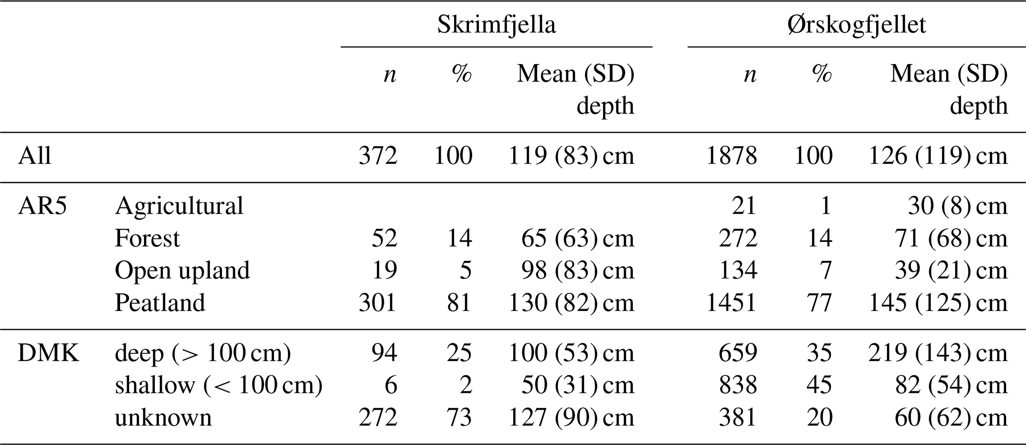
Table 2 Selected attributes of the peat depth datasets at Skrimfjella and Ørskogfjellet. The first row summarizes all 10 m cells, while subsequent rows stratify the dataset by AR5 land class and DMK peat depth class.

DSM products have much more value when their predictions are accompanied by uncertainty estimates, and all DSM should strive to assess uncertainty (Arrouays et al., 2020; Wadoux et al., 2020) and evaluate uncertainty estimates (Heuvelink and Webster, 2022). Therefore, we produced prediction intervals with quantile regression forests (Meinshausen, 2006), and used the same spatial cross-validation to evaluate the prediction interval coverage probability (Shrestha and Solomatine, 2006). The quantile regression forests were trained with the predictor configuration that showed the highest performance at each site, and we extracted 90 % prediction intervals.

2.5.3 Model interpretation

We quantified global variable importance (predictor influence across all locations) and examined partial dependence plots (curves of fitted relationships) for the best-performing predictor configuration at each site. Both are useful for understanding the mechanisms behind the model's predictions and the roles of the predictors in the model.

For both sites, we interpreted a model trained on a non-collinear subset of variables from the best performing predictor configuration – because correlation between predictors degrades variable importance metrics (Strobl et al., 2008; Biau and Scornet, 2016) and can produce misleading visualizations of predictor–outcome relationships (Biecek and Burzykowski, 2021; Dwivedi et al., 2023). Specifically, we eliminated variables from the best performing predictor configuration to obtain a set with no pairwise Pearson correlation coefficient above 0.7 (an arbitrary but conventional threshold for this purpose). Thus, highly correlated sets of variables are represented by a single variable for the purposes of model interpretation.

We calculated variable importance with the vip R package (v.0.4), by three different methods: FIRM, permutation, and Shapley (Greenwell and Boehmke, 2020). FIRM values measure the flatness of the partial dependence plot, permutation values measure the decrease in model performance when the predictor is permuted, and Shapley values are aggregated from local, game-theoretical measures of variable importance (Greenwell and Boehmke, 2020). Since FIRM reflects the flatness of the partial dependence plot, it captures functional complexity rather than overall predictive impact. Permutation values were obtained from ten iterations, with root mean square error as the performance measure.

We calculated partial dependence with the pdp R package (v.0.8; Greenwell, 2017). For the six most important variables, we plotted partial dependence to show the average effect of the predictor on the outcome and individual conditional expectations to show variation in the effect across observations (Goldstein et al., 2015). Non-parallel individual conditional expectation lines indicate the presence of interactions between predictors.

3 Results

Our point measurements of peat depth (all sources) produced aggregated depths for 372 cells or 2.4 % of AR5 mire area at Skrimfjella, and 1878 cells or 1.2 % of AR5 mire area at Ørskogfjellet. Approximately 80 % of these 10 m cells were within AR5 mires, and the remainder in forest, open upland, or farmland (Table 2). DMK peat depth had higher coverage at Ørskogfjellet than at Skrimfjella (80 % versus 27 % of cells not unknown), and at Ørskogfjellet the deep and shallow classes showed a larger difference in measured depth. Overall, mean peat depths were similar at Skrimfjella and Ørskogfjellet (119 cm versus 126 cm) but the distribution was more right-skewed at Ørskogfjellet (Fig. 2).

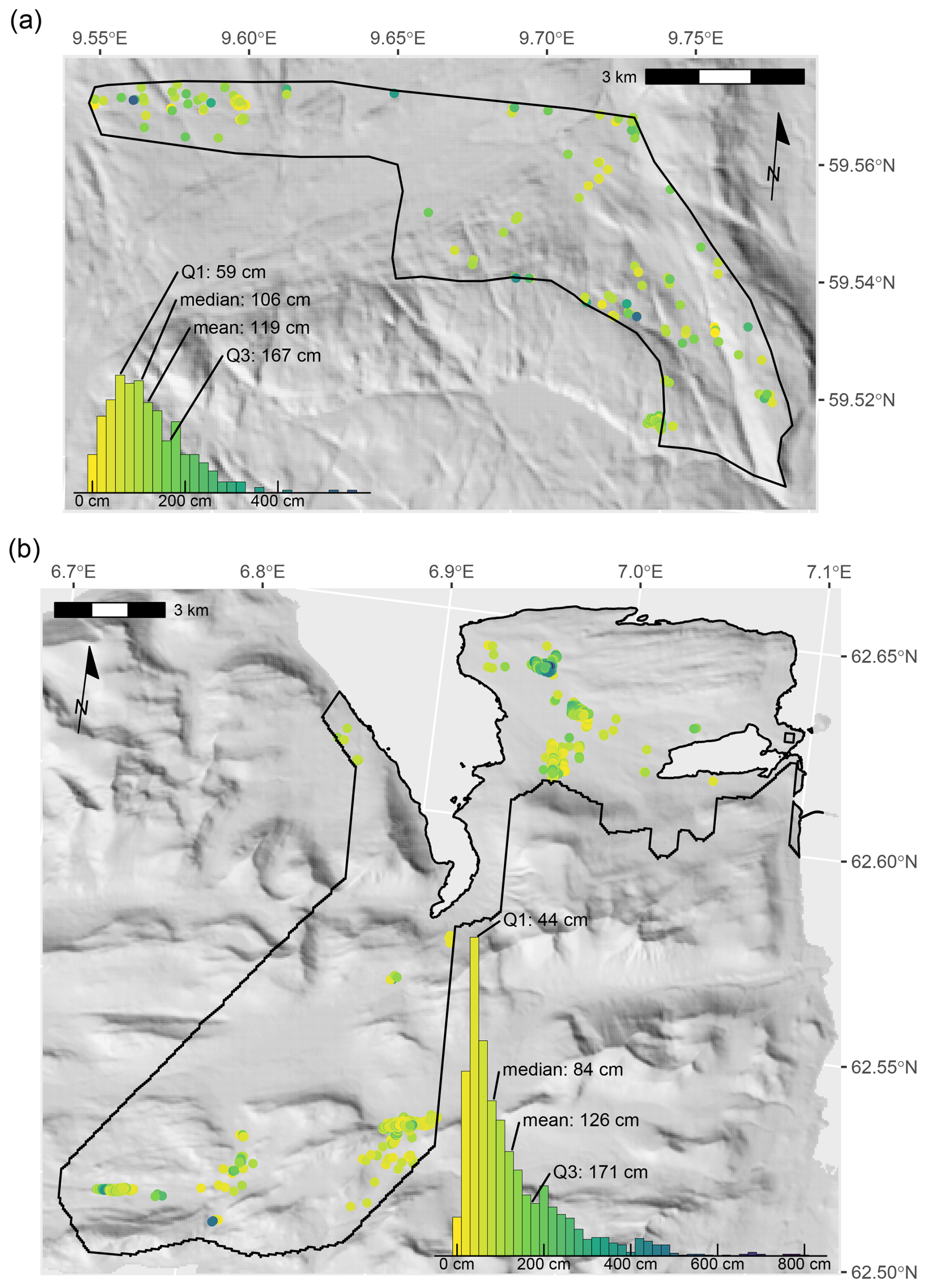
Figure 2 Spatial and statistical distributions of mean peat depth in 10 m cells at Skrimfjella, N=372 (a) and Ørskogfjellet, N=1878 (b). Terrain is visualized with a hillshade with slope 45° and azimuth 225°. Terrain data are from the Norwegian Mapping Authority under the Creative Commons Attribution 4.0 International license (https://creativecommons.org/licenses/by/4.0/, last access: 20 September 2024) © Kartverket.

3.1 Model performance

None of the models were able to predict peat depth across the study areas with high accuracy (Fig. 3). For Skrimfjella, the best model achieved a concordance correlation coefficient of 0.30, an R² of 0.34, and a mean absolute error of 60 cm. For Ørskogfjellet, the concordance correlation coefficient was 0.39, R² was 0.33, and mean absolute error was 56 cm, so the best model at Ørskogfjellet was slightly more accurate than the best model at Skrimfjella. These values were derived from kNNDM spatial cross-validation with 20 folds at Skrimfjella and 10 folds at Ørskogfjellet.

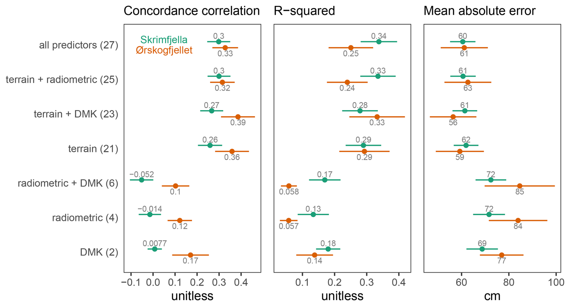
Figure 3 Performance of peatland depth models with different predictor configurations, evaluated via spatial cross-validation. Parentheses denote the number of variables in each predictor configuration, and point estimates are shown ± their standard error.

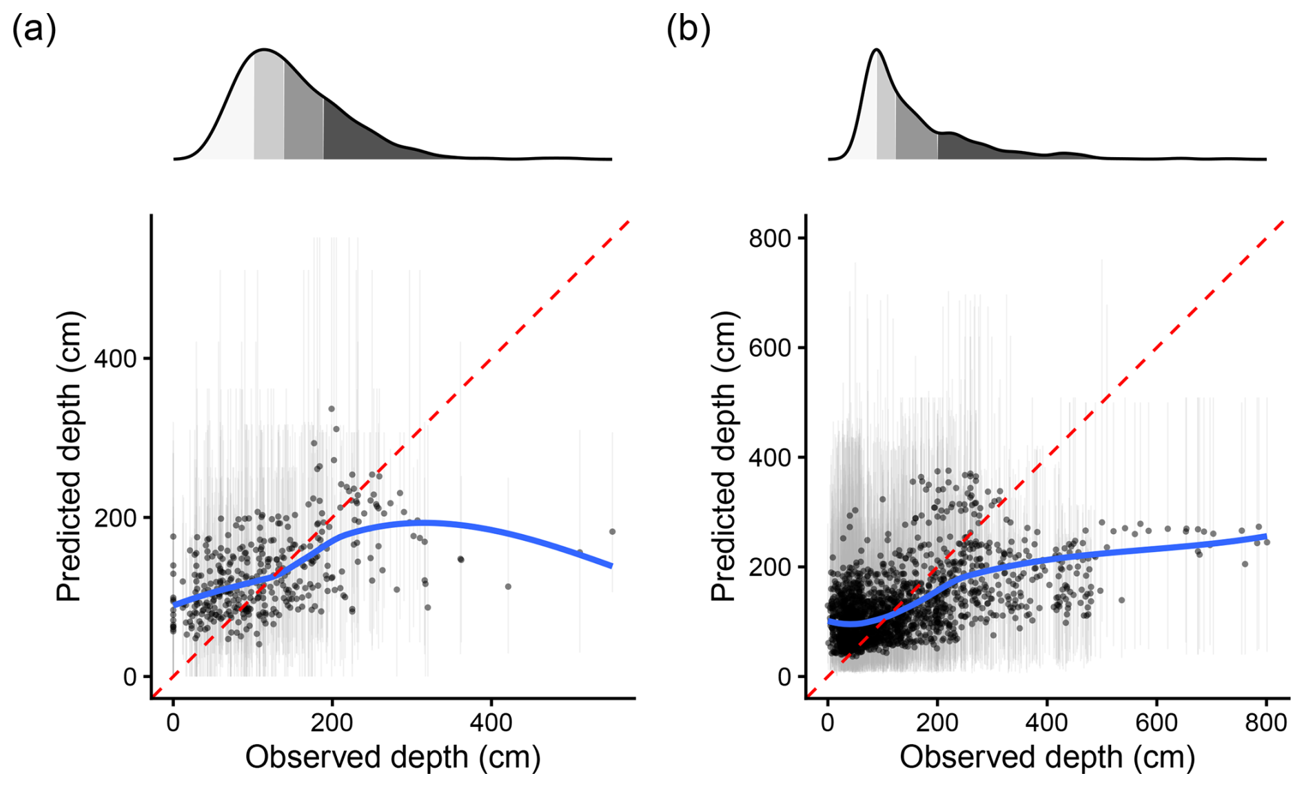
Figure 4 Calibration plots for the best-performing models at Skrimfjella (a) and Ørskogfjellet (b), with predictions and 90 % prediction intervals (grey vertical lines) from spatial cross-validation. Points have transparency to show overlap. Blue lines are local polynomial regressions and the red dashed line in each panel shows the 1:1 line. Marginal distributions (top) are shaded by quartile.

For Skrimfjella, the best predictor configuration was all predictors, followed closely by terrain + radiometric (Fig. 3). The terrain configuration outperformed the radiometric configuration by 0.27 in concordance correlation coefficient (p<0.001; Table C1), by 0.16 in R² (p=0.190; Table C2), and by 10 cm in mean absolute error (p=0.038; Table C3). The terrain + DMK configuration outperformed the radiometric + DMK configuration by 0.32 in concordance correlation coefficient (p<0.001; Table C1), by 0.11 in R² (p=0.605; Table C2), and by 11 cm in mean absolute error (p=0.011; Table C3).

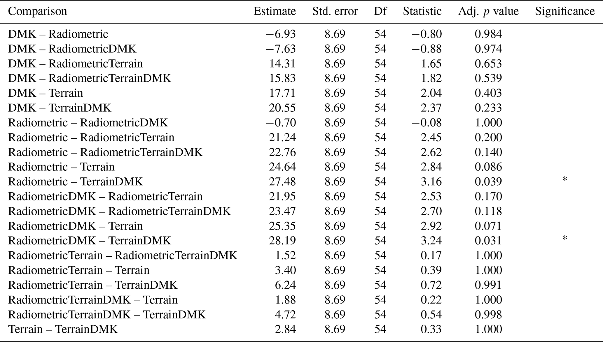
For Ørskogfjellet, the best predictor configuration was terrain + DMK, followed by terrain (Fig. 3). Adding radiometric predictors to these configurations slightly worsened model performance. The terrain configuration outperformed the radiometric configuration by 0.24 in concordance correlation coefficient (p=0.068; Table C4), by 0.24 in R² (p=0.004; Table C5), and by 25 cm in mean absolute error (p=0.086; Table C6). The terrain + DMK configuration outperformed the radiometric + DMK configuration by 0.28 in concordance correlation coefficient (p=0.015; Table C4), by 0.27 in R² (p<0.001; Table C5), and by 28 cm in mean absolute error (p=0.031; Table C6).

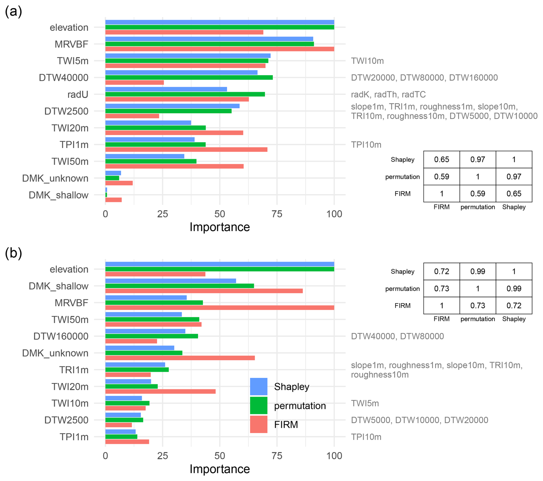
Figure 5 Global variable importance in the best-performing models at Skrimfjella (a) and Ørskogfjellet (b), as measured by three different metrics: Shapley values, permutation importance, and the Feature Importance Ranking Measure (Greenwell and Boehmke, 2020). Variables removed due to collinearity are shown to the right of the variable with which they are most correlated. Spearman rank correlations between the three metrics at each site are displayed in matrices.

The best models at both sites overpredicted shallow peats and strongly underpredicted very deep peats (Fig. 4). The mean error (bias) of these models was 10 cm at Skrimfjella and −4 cm at Ørskogfjellet. Although the prediction intervals from the quantile regression forests were wide, they were well calibrated. At Skrimfjella, the prediction interval coverage probability was 92 %, and at Ørskogfjellet it was 84 % (both compared to the target value of 90 %). Observations outside of the prediction intervals showed no obvious spatial pattern.

3.2 Model interpretation

For the purpose of model interpretation, the all predictors configuration for Skrimfjella was reduced from 27 variables to 11 non-collinear variables, by removing one of the variables in each highly-correlated pair. Similarly, the terrain + DMK configuration for Ørskogfjellet was reduced from 23 variables to 11 non-collinear variables. The permutation and Shapley methods of variable importance showed high Spearman rank correlation at both sites, while the FIRM method ranked variable importance differently (Fig. 5).

3.2.1 Variable importance

At both sites, elevation and Multi-Resolution Valley Bottom Flatness were important predictors (Fig. 5). At Skrimfjella these two predictors were of similar importance, while at Ørskogfjellet elevation had higher predictive impact (permutation and Shapley) but lower functional complexity (FIRM) than Multi-Resolution Valley Bottom Flatness. DMK was also important – the shallow class in particular – but only at Ørskogfjellet. Some realizations of the hydrological predictors Topographic Wetness Index and Depth-to-Water showed considerable importance, while others showed little – with no clear consistency between sites. At both sites, the most important hydrological predictors were more important than the simple terrain indices slope, Terrain Ruggedness Index, Topographic Position Index, and roughness. At Skrimfjella, the radiometric predictor uranium ground concentration – which was highly correlated with all other radiometric variables – showed moderate importance.

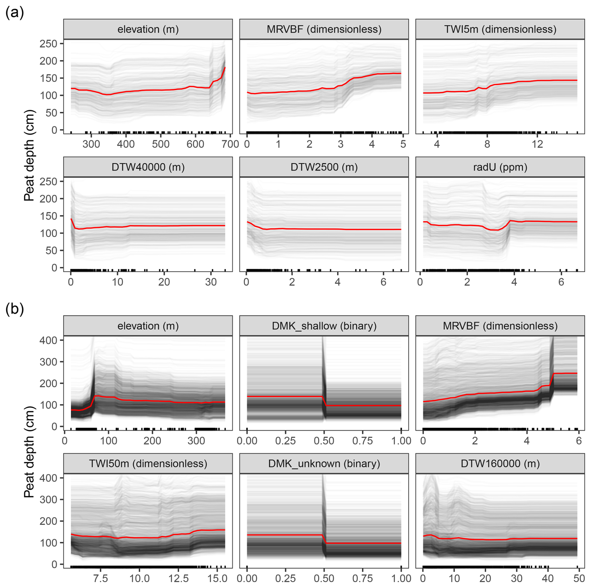
Figure 6 Partial dependence plots of the six most important variables in the best-performing models at Skrimfjella (a) and Ørskogfjellet (b). The average effect of the predictor on the outcome (red line) overlays the individual conditional expectations, which show the variation in the effect across observations (grey lines). The variables' training data distributions are indicated with rug plots along the x-axes.

3.2.2 Partial dependence

Many of the most important predictors in the best performing models showed non-monotonic effects on peat depth (Fig. 6). At Ørskogfjellet, for example, increasing elevation was predictive of deeper peat up to about 75 m a.s.l., after which a further increase was predictive of shallower peat. At Skrimfjella the partial dependence on elevation had the opposite shape but covers a higher elevation range, with the shallowest peats predicted around 350 m a.s.l. TWI50m at Ørskogfjellet and DTW4000 and uranium ground concentration at Skrimfjella were other predictors that showed non-monotonic associations with peat depth. The radiometric predictor in particular displayed an idiosyncratic effect, with a marked dip in predicted depth at intermediate values of uranium ground concentration. On the other hand, the partial effects of some important predictors were more straightforward. The partial dependence on Multi-Resolution Valley Bottom Flatness was quite similar across sites, with the deepest peats predicted in the very flattest valley bottoms. Also, TWI5m and DTW2500 at Skrimfjella showed monotonically positive and negative predictive effects, respectively.

Individual conditional expectation lines indicated some interactions between predictors (Fig. 6). For example, the positive association of depth with elevation at Ørskogfjellet was larger for some observations than others; depth increases ranged 40–100 cm over the same elevation gain. Similarly, individual conditional expectations along uranium ground concentration at Skrimfjella were non-parallel, with some locations showing decreasing peat depth predictions (unlike the average effect). Nevertheless, most individual conditional expectations were approximately parallel, so the average effects of the predictors are mostly representative of their overall effects.

4 Discussion

4.1 Can we improve Norway's peat depth maps?

4.1.1 Remotely sensed variables are weak predictors of peat depth

Our ability to predict peat depth in the study sites based on terrain and radiometric data was limited. Mean absolute errors of 60 and 56 cm at the two sites – relative to mean depths of 119 and 126 cm – illustrate the practical limitations of these maps. Since any given 10 m cell will miss by about 60 cm, applications requiring detailed peat depth in a small area (e.g., <1 ha) would benefit from measuring depth on the ground rather than relying on the DSM alone.

Although model performance was limited, we improved on the best available map of peat depth (DMK depth class), which is based on field measurements only. This highlights the general value of remotely sensed data, whose complete coverage can improve maps even when their association with the variable of interest is weak (Mulder et al., 2011). Since remotely sensed data are widely available, improvements to soil maps as shown here are readily achievable at low cost (Minasny et al., 2019).

DMK peat depth classes were a worse predictor of peat depth than our models even though we calibrated them with the same data (Fig. 3). If we had taken the DMK peat depth classes at face value and assumed depths according to their class definitions (<1, >1 m), they would have performed worse and the advantage of the DSM would be greater. The advantage of the DSM was not large in absolute terms (9 and 21 cm improvements in mean absolute error), but it explained much more of the variation in depth (improvements in R² of 0.16 and 0.19). We attribute this result to the poor spatial and thematic resolution of DMK peat depth, which precludes a robust correlation with peat depths.

The accuracy of our mapping could have been improved with a spatially explicit approach like regression kriging. However, residuals of the RF predictions showed weak spatial structure at Skrimfjella, and only up to a range of 150 m at Ørskogfjellet. Therefore, the improvement from regression kriging would be small overall and limited to parts of the maps close to measurements.

4.1.2 Similar error but less explanatory power in Norwegian peatlands

Compared to other studies using terrain and radiometric data to predict peat depth, our models explained less variability in peat depth (R²) but generally produced better or comparable error magnitude (mean absolute error or root mean square error; Wadoux et al., 2022). It is important to keep in mind that differences in peat depth distributions, spatial scales, and evaluation methods make direct performance comparisons precarious. For example, R² is sensitive to high leverage, extreme values, so it will evaluate a right-skewed distribution differently than a symmetrical distribution. We evaluated our models with respect to the explicit purpose of creating peat depth maps across the study areas, but not all studies tailored evaluation to match an explicitly formulated problem (Milà et al., 2022).

Gatis et al. (2019) used similar predictors and the same spatial grain, finding a much stronger relationship between predicted and observed peat depth (R²=0.68). Although their random evaluation data partition could make performance estimates too optimistic (Roberts et al., 2017; Wadoux et al., 2021), the confounding effect of spatial structure is probably small because they used linear regression and few predictors, so their model had limited opportunity to overfit to the spatial structure in peat depth. The most salient difference in Gatis et al. (2019) compared to our study is the character of the study area. They study a flatter area with a higher proportion of peatland cover, and their peatland is primarily blanket bog. The peat surface of a blanket bog is tied more closely to its underlying topography than the peat surface of raised bogs or fens (Lindsay, 2016b), which may make blanket bog depth easier to predict. The predominance of fens and smaller peatland extent may have contributed to worse performance in our study.

Marchant (2021) examined a subset of the area studied in Gatis et al. (2019) at 100 m resolution, using splines to relax linearity between radiometry/terrain and peat depth. He found that potassium ground concentration alone predicted peat depth with much higher concordance than our models (concordance correlation coefficient = 0.76) and that elevation alone produced comparable performance (concordance correlation coefficient = 0.27). The root mean square error from these univariate models was 46–68 cm (cf. 78 and 75 cm for Skrimfjella and Ørskogfjellet).

Koganti et al. (2023) had a peat depth distribution and predictors similar to ours, but at much smaller spatial grain and extent. Their training and validation points are closer than the range of spatial autocorrelation in peat depth, so our results are best compared to their non-spatial models. They accounted for more variability in peat depth (adjusted R²=0.71) but had larger errors (RSME = 110 cm). The linear regression models in Koganti et al. (2023) produced negative predictions, and it is unclear whether the values quoted above include these. If we disregard the negative predictions, their model showed the same pattern as ours in overpredicting shallow peats and underpredicting deep peats, although their underprediction was less severe. An important difference between Koganti et al. (2023) and our study (besides spatial scale) is that they measured radiometrics on the ground, rather than using airborne survey data. Thus, the footprint of their detector was smaller and they captured variation in radiation at finer scales.

4.1.3 Asymmetries in depth predictions for land use planning and carbon accounting

Our models erred most for the deepest peats (Fig. 4). Where overprediction occurred, the error was smaller. This is not unexpected for the right-skewed distributions of peat depth, but it has implications for potential users of the maps. For example, it makes the maps more suited for “red-lighting” than “green-lighting” peatland conversion (assuming depth is the determinative factor). Identifying the deepest peats will require additional field work in candidate areas – where candidate areas could be defined by some upper quantile of predicted depth.

4.2 Which variables predict peat depth?

4.2.1 Airborne radiometrics do not predict Norwegian peat depth

Radiometric data had little to no predictive value at either site (poor performance of radiometric configuration), although they did contribute to the best model at Skrimfjella (marginal improvement in all predictors configuration compared to terrain + DMK). These results contrast with earlier studies that found that radiometrics were useful predictors of peat depth (Keaney et al., 2013; Gatis et al., 2019; Koganti et al., 2023; Pohjankukka et al., 2025). The bedrock is more homogeneous at Ørskogfjellet than at Skrimfjella, so uneven radiogenesis is not a good explanation for the higher predictive value of radiometric variables at Skrimfjella (Beamish, 2014; Reinhardt and Herrmann, 2019). All four radiometric variables were highly correlated within the peatland parts of our study sites, so there could be no large differences in their predictive value. This contrasts with Koganti et al. (2023), who found that radiometric total count and potassium ground concentration were better predictors than thorium or uranium ground concentration.

We suspect that the primary reason for the poor predictive value of the radiometric data was the large footprint of the detector in the airborne survey. With an average flight altitude of 75 m, less than half of the radiation reaching the detector comes from inside the 100 m diameter circle directly below it (Beamish, 2016; Beamish and White, 2024). The rest of the measured activity integrates a much wider area. For comparison, empirical variograms of peat depth at Skrimfjella and Ørskogfjellet showed no spatial autocorrelation beyond 50 and 75 m (among GPR data) or 110 and 230 m (among 10 m cells). Basically, the airborne radiometric data will not capture large variation over short (<100 m) distances; the instrument's field of view has a large smoothing effect on the data (Beamish, 2016; Reinhardt and Herrmann, 2019). Different landforms and the changes they cause in the geometry between the radioactive source and the detector can also distort airborne measurements (Reinhardt and Herrmann, 2019).

Studies comparing airborne and ground radiometric surveys confirm that they are poorly correlated in low-activity areas like peatlands (Kock and Samuelsson, 2011; Karjalainen et al., 2025). Karjalainen et al. (2025) found that ground-based measurements predicted peat depth better than airborne measurements. Nevertheless, a large radiometric footprint did not prevent strong associations with peat depth in Gatis et al. (2019) and Marchant (2021), perhaps because the extensive blanket bog landscape in these studies has more gradual changes in depth (Lindsay, 1995). We are unsure whether short-range depth changes explain the weak associations that Siemon et al. (2020) found in a large raised bog.

Another possible reason for the poor predictive value of the radiometric data could be that other physical parameters influencing the amount of intercepted radiation varied too much within sites. Initial source strength, soil moisture, bulk density, and porosity all affect the amount of radiation that reaches the detector (Beamish, 2013; Reinhardt and Herrmann, 2019). Therefore, variation in these parameters could have masked the relationship between peat depth and radiometric data. This makes physical modeling of peat depth from radiometric data an undetermined problem. We chose the Ørskogfjellet site in part because it has a relatively homogeneous bedrock, which should reduce the variation in initial source strength. Soil moisture, bulk density, and porosity, however, are not easily measured across landscape scales and were assumed to be homogeneous. Uneven snow cover and air moisture during the Ørskogfjellet radiometric survey may also have masked the soil signal in these data, as Ofstad (2015) reports large variation in weather conditions. If maps of these other physical parameters at the time of the radiometric survey were available and included in the model, the predictive value of radiometric data might improve, but this is not a practical solution for digital soil mapping of peat depth.

We do not believe that the poor predictive value of the radiometric data in this study was caused primarily by full attenuation of radioactivity. The RF algorithm's flexibility means that radiometrics could be used for shallower peats if they provided predictive value for that part of the depth distribution, but there is no evidence of that in our results. In the partial dependence plot of uranium ground concentration at Skrimfjella, the expected negative relationship between depth and uranium ground concentration cannot be found by ignoring the left (highly attenuated) side of the distribution (Fig. 6). More than a quarter of the peats in each of our study areas were less than 60 cm deep, and full attenuation is unlikely for these (Beamish, 2013).

Although we do not believe full attenuation is the primary reason for poor performance in our study, it may limit peat depth mapping under other circumstances. First-principle calculations suggest that radiation should be 90 % attenuated after about 50–60 cm of typical, wet peat or 85 cm of unnaturally dry peat (Beamish, 2013; Beamish and White, 2024), and some field tests support these values (Billen et al., 2015). It is remarkable that particular studies detected radiation differences up to several meters deep (Gatis et al., 2019; Koganti et al., 2023), but these may be the exceptions rather than the rule. Perhaps relatively deeper water tables in these study sites (blanket bog, drained fen; Price et al., 2016) contributed to better penetration.

4.2.2 Terrain-based variables can predict peat depth

At both our sites, lidar-derived terrain variables predicted peat depth much better than radiometric variables (Fig. 3). This is consistent with the findings of Pohjankukka et al. (2025), who mapped peat depth classes at 50 m resolution across Finland.

At both our sites, elevation was the most important predictor, and peat depth showed non-monotonic responses to changes in elevation (Figs. 5 and 6). We believe that the idiosyncratic elevational relationships we detected are mostly not generalizable beyond the study areas, because we see no simple mechanism (e.g., via climate) to explain the observed patterns. For example, the increase in peat depth from 350 to 700 m a.s.l. at Skrimfjella is opposite to the general pattern of deeper peats in lowland than upland Norway (Lyngstad et al., 2023). Moreover, elevation at Ørskogfjellet seems to interact with other variables (non-parallel individual conditional expectation lines), complicating its interpretation. Relationships between elevation and peat depth have previously shown opposite shapes in different areas (Finlayson et al., 2021). Nonetheless, a relationship that is not generalizable beyond the mapping area is still useful for DSM, as long as it is evaluated to demonstrate its robustness for the predictive task (e.g., through kNNDM spatial cross-validation).

One interesting feature of the elevational relationships we found may be generalizable: a steep increase in peat depth near the marine limit after the last ice age. At Ørskogfjellet, the marine limit is about 75 meters above today's sea level (Geological Survey of Norway; Høgaas et al., 2012), where the partial dependence plot of elevation shows a sharp increase in peat depth. In areas under the marine limit there has been less time for peat accumulation since the ice sheets retreated, and it is plausible that this makes peats there shallower, all else being equal. This hypothesis is supported by similar findings at a coarser scale in the Hudson Bay Lowlands, where a strong positive relationship between peat depth and distance from the coast can be explained by isostatic uplift and time since peat initiation (Li et al., 2025). The same has been reported for Finland (Pohjankukka et al., 2025). We cannot evaluate this effect at Skrimfjella, where the marine limit is below our study area (at 175 m a.s.l.).

Another influential terrain-based predictor was Multi-Resolution Valley Bottom Flatness (Fig. 5). Unlike elevation, it showed a monotonic effect on peat depth: greater valley bottom flatness was always associated with increases in peat depth (Fig. 6). Delineating a valley bottom involves ambiguity, but the Multi-Resolution Valley Bottom Flatness index is a pragmatic approach that considers a location a valley bottom if it is sufficiently low and flat at a particular scale (Gallant and Dowling, 2003). The multiscale nature of the index allows small elevated but flat areas (including saddles) to be characterized as having high valley bottom flatness (Gallant and Dowling, 2003). Our results suggest that Multi-Resolution Valley Bottom Flatness is a robust indicator of high water tables (and peat accumulation) over millennial time scales, corroborating other studies (Rudiyanto et al., 2018; Deragon et al., 2023).

Other terrain-derived predictors with predictive value in our study are hydrological (Topographic Wetness Index and Depth-to-Water). Notably, slope was inferior to (at Ørskogfjellet) or highly correlated with (at Skrimfjella) these hydrological indices. Mappers of peat depth should not assume that slope is the best terrain-derived predictor, despite its prevalence in the literature (Pohjankukka et al., 2025). Wetter locations (high Topographic Wetness Index and low Depth-to-Water) were generally associated with deeper peat, but these relationships were not as strong or consistent as with Multi-Resolution Valley Bottom Flatness (Figs. 5 and 6). The optimal scale for Topographic Wetness Index and Depth-to-Water varied, and likely depends on both the dominant peat formation processes and the typical size of peatland features in a landscape. Including multiple scales of these variables allows the model to capture different hydrological mechanisms or patterns operating at different spatial scales.

4.2.3 Legacy depth maps have inconsistent predictive value

DMK peat depth class proved an inconsistent predictor of peat depth. At Skrimfjella, it barely improved model performance (Fig. 3). At Ørskogfjellet, it increased performance more, and both indicator variables (shallow and unknown) were among the most important in the model (Fig. 5). We suspect the discrepancy between sites is due to different levels of effort and coverage during the historical surveys; more lowland peatland near agriculture at Ørskogfjellet may have caused more purposeful surveying. This is evidenced by the fact that 73 % of the cells measured at Skrimfjella had unknown depth in DMK, compared to 20 % at Ørskogfjellet. Interactions between DMK and other variables also underline the inconsistency of DMK depth maps, even within a site. For example, shallow peat classification in DMK sometimes increased rather than decreased predicted depth at Ørskogfjellet.

4.3 Implications for digital soil mapping of peat depth

The performance gap between the best models and the DMK models shows that DSM of peat depth has value in Norway. Where calibrating measurements are available, better maps than DMK peat depth class can be produced at low cost. Moreover, DSM can make the production of maps transparent, reproducible, and updatable. We can apply the same approach across different areas and make maps with full spatial coverage, continuous values, and validated uncertainty. The large difference in coverage and quality of DMK peat depth at Skrimfjella versus Ørskogfjellet underlines these advantages.

4.3.1 Peat depth measurements should be organized

High-quality DTMs are available for mainland Norway, which makes peat depth measurements the critical training data needed for DSM. Better infrastructure to make depth measurements findable, accessible, interoperable, and reusable would help DSM and other applications. Geoportal access and data exchange standards, such as those developed in Natural England (2023) for peat surveys, are important. Peat depth is quick and easy to measure, so integrating its measurement into existing national field programs, like Norway's spatially representative nature monitoring or national forest inventory, would be helpful (although not sufficient for regional or local mapping). Low-altitude, drone-mounted GPR may prove an efficient approach for collecting many, accurate depth data in a landscape, by combining the advantages of airborne deployment and active sensing (Pelletier et al., 1991; Ruols et al., 2023).

4.3.2 Spatial scale affects model performance and utility

Peat depths typically vary over short distances (e.g., <1 m), so mapping at 10 m resolution implies that the map will compress much of the fine-scale variation. Terrain–depth relationships might be stronger at finer resolution than 10 m, especially considering the hummock–hollow microtopography of many peatlands (Rydin et al., 1999; Lindsay, 2010). Therefore, it may be advantageous to model peat depth at 1 m resolution – even if land use planning and carbon accounting do not operate at such fine scale.

To define a spatial extent for a particular DSM, kNNDM can be used to investigate how far the map can extend beyond a set of point measurements; if the sample-to-prediction nearest neighbor distribution cannot be simulated by any set of cross-validation folds, then the extent is too expansive (Meyer and Pebesma, 2022; Linnenbrink et al., 2024). However, the tradeoff between multiple small-extent DSM and fewer large-extent DSM needs research. Bohn and Miller (2024) advocate for bottom-up stitching of local DSM, and for peat depth we assert that these should at least stay within peatland regions (or “supertopes”), where the composition of mesotopes is similar – e.g., regions dominated by raised bogs versus regions dominated by sloping fens (Moen, 1999; Joosten and Clarke, 2002). Depth varies systematically between bogs and fens (Lindsay, 2016b), between peats formed by terrestrialization versus paludification (Buffam et al., 2010), and probably along other axes of peatland typology. Therefore, DSM is more likely to uncover consistent predictor–depth relationships within peatland regions than across them.

4.3.3 Machine learning approaches can build on success

The DSM literature and our results support using flexible machine learning algorithms like RF to predict peat depth. RF avoids negative predictions (cf. Koganti et al., 2023) and produces good uncertainty estimates (our study; Vaysse and Lagacherie, 2017; Takoutsing and Heuvelink, 2022). As depth data become more abundant, pixel-based learners may be surpassed by deep learning approaches like convolutional neural networks. The success of Multi-Resolution Valley Bottom Flatness as a predictor of peat depth demonstrates that multiscale spatial patterns matter for peat depth, and convolutional neural networks are designed to learn such patterns (Borowiec et al., 2022). The kind of relationship described in Buffam et al. (2010), where peat depth in basins related to terrain slope at the basin edge, is also something a convolutional neural network could learn. However, since this approach is data-hungry, we should build soil knowledge into the DSM where we can (Minasny et al., 2024b).

4.3.4 Peat extent and depth should be mapped together

Finally, we would like to highlight briefly the need for peatland extent mapping and peat depth mapping to be better integrated. Since peatland extent is defined by non-zero peat depth (the specific threshold varies by definition; Minasny et al., 2024a), the lateral and vertical dimensions are fundamentally linked. The goal, therefore, should be a unified prediction framework for extent and depth. Research is needed to determine whether it is better to parameterize a single model of peat depth across a full landscape, or to break down the problem into a hurdle model by classifying zero depth and then regressing non-zero depths. Though peatland definitions may encourage reducing continuous depth predictions to arbitrary classes, we caution against this practice (as in Ivanovs et al., 2024; Karjalainen et al., 2025).

5 Conclusions

This study demonstrates that digital soil mapping at 10 m resolution can improve upon existing peat depth maps in Norway, though the strength of the relationship between available predictors and peat depth remains limited. Our findings show that terrain-derived variables, particularly elevation and Multi-Resolution Valley Bottom Flatness, provide predictive value for peat depth mapping within peatland extents. In contrast, airborne radiometric data showed little to no predictive value at either of two study sites, possibly because of the large footprint of airborne spectrometers relative to the fine-scale variation in peat depths.

The best models achieved mean absolute errors of 56–60 cm against mean depths of 119–126 cm, and explained approximately one-third of the variation in peat depth across landscapes with aggregate peatland areas of 1.5–15.3 km². Though field measurements remain necessary for local, detailed assessments of peat depth, digital soil maps at 10 m resolution can provide valuable information for landscape-scale planning and regional carbon assessments. The models' tendency to underpredict the deepest peats has important practical implications, making them more suitable for precautionary screening than comprehensive coverage. As Norway and other nations pursue nature-based climate solutions, these findings highlight both the potential and limitations of remote sensing for peatland carbon mapping.

Appendix A

Table A1 Attributes of the radiometric surveys, as reported in Baranwal et al. (2013) and Ofstad (2015).

Appendix B

B1 Peat depth sample selection

B1.1 Skrimfjella

At Skrimfjella, we used the eSample function in the iSDM R package (v.1.0) to stratify our sample across elevation, slope, and potassium concentration. This function defines the environmental space as a two-dimensional convex hull around the PCA-ordinated data, then creates a regular grid across that space, and lastly finds for each grid cell the datum that is nearest (Hattab et al., 2017). We set a target sample size of 100, excluded the top and bottom percentile from the convex hull, and eSample returned 105 raster cells.

B1.2 Ørskogfjellet

At Ørskogfjellet, we first determined a minimal sample size that would adequately capture the slope and radiometric properties (potassium, thorium, uranium, and total count) of the entire AR5 mire area (Saurette et al., 2023). Specifically, we identified an elbow point in a curve of similarity between sample and population (Malone et al., 2019). For a sequence of sample sizes (50–500) (ten replicates each, drawn by conditioned latin hypercube sampling; Minasny and McBratney, 2006; Roudier, 2011), we calculated the mean Kullback–Leibler divergence between sample and population distributions (Malone et al., 2019; Saurette et al., 2023). Then we fitted an asymptotic regression of mean divergence on sample size, and found that the curve reached 95 % of the fitted asymptote at a sample size of 160.

To choose 160 locations, we performed feature space coverage sampling, implemented using the kmeans function in base R and the rdist function in the fields package (v.14.2; Nychka et al., 2025). Feature space coverage sampling chooses locations that are closest to cluster centers in standardized predictor space (Brus, 2019). This approach has been found to produce higher accuracy in RFs than conditioned latin hypercube sampling (Wadoux et al., 2019; Ma et al., 2020). Feature space coverage sampling works best when all dimensions are important predictors of the outcome (Wadoux et al., 2019), and we used the same five predictors that we used to choose sample size: slope and four radiometrics.

We adjusted the feature space coverage sampling to ensure that locations were accessible within time constraints, and assessed how this changed our sample from an ideal feature space coverage sample. Adjusting for accessibility is justified because the smaller sample size that would result if accessibility were ignored can degrade model accuracy as much or more as deviations from ideal sampling designs (Wadoux et al., 2019; Ma et al., 2020). To adjust, we first restricted the sampling population to AR5 mire areas that were within an arbitrary cost distance of publicly accessible roads. Cost distance was calculated using GRASS's r.walk function, with friction costs defined by AR5 land classes (GRASS Development Team, 2022). After creating a feature space coverage sample with this restriction, we also inspected a map of the sample and substituted 16 inaccessible locations with accessible locations from the same or a nearby cluster. Our two accessibility adjustments increased the distance in standardized predictor space between sample locations and cluster centers by 78 % (compared to the ideal sample), but distance in our sample was still only 46 % of the mean distance to cluster centers – i.e., accessibility did not force locations far from cluster centers relative to the size of the clusters.

B2 Depth measurements

B2.1 Peat probing

We navigated to the centers of the raster cells in our samples using handheld (Skrimfjella) or real-time kinematic (Ørskogfjellet) global navigation satellite system (GNSS) receivers. We dampened the effect of outlying measurements by probing three times at each location (Parry et al., 2014), at the vertices of a centered triangle with 2 m (Skrimfjella) or 4.5 m (Ørskogfjellet) sides. We used changes in resistance to indicate the base of the peat column. Probe locations were adjusted up to 20 cm if the base of the peat column seemed to be blocked by an obvious artifact, like a buried rock. Where the peat column was deeper than the extendable probe could be manually inserted and extracted by a pair of operators, we recorded a right-censored result (one at Skrimfjella, five at Ørskogfjellet).

B2.2 Ground-penetrating radar

We performed GPR surveys in three subjectively chosen peatlands at Skrimfjella and in areas with a high density of sampled raster cells at Ørskogfjellet. We used the Malå ProEx GPR system (Guideline Geo AB, Sweden) with a GNSS-enabled control unit connected to a 500 MHz shielded antenna mounted in a plastic sledge (transmitter–receiver separation 0.18 m, trace frequency 10 Hz). For some transects at Ørskogfjellet we substituted a 100 MHz Malå rough terrain antenna (transmitter–receiver separation 2.2 m, trace frequency 5 Hz), because the lower frequency antenna gives greater penetration depth. In all cases the system was towed by a walking GPR operator.

GPR traces were recorded along zigzag (Skrimfjella) or snaking (Ørskogfjellet) transects. At Ørskogfjellet, transects were predetermined to pass through the centers of sampled raster cells, and we marked these precisely with flags to guide the GPR operator. A GPR records the time taken for a radio wave to travel from the transmitter to a reflector and back to the receiver, and the velocity of the wave varies with properties of the peat column. Therefore, wave velocity has to be calibrated to convert travel time to peat depth, and we probed peat depth along the transects.

We processed the GPR data with Reflex2DQuick (v.3.0; Skrimfjella) or REFLEXW (v.8.5; Ørskogfjellet) software (Sandmeier Scientific Software, Germany). We applied a time-zero correction, a dewow filter, and a gain filter based on observed energy decay. With Ørskogfjellet data, we also applied a bandpass filter and a dynamic correction that accounts for the non-vertical wave path between offset transmitter and receiver antennas. The latter is important for the rough terrain antenna, where the antenna separation is comparable to typical peat depths. From the processed radargrams, we picked travel times from strong reflectors that we interpreted as the base of the peat column.

We used picks near probed depths to calibrate wave speed velocity – separately for each site. Calibration data were created by matching marked trace locations to a corresponding depth probe (Skrimfjella), or by a spatial join that identified interpreted traces and depth probes within 2 m of each other (Ørskogfjellet). We had sufficient calibration point density to avoid bias in wave velocity as a major source of error (Rosa et al., 2009): 46 calibration points along 3.5 km of interpretable traces at Skrimfjella, and 78 along 7.8 km at Ørskogfjellet. We fitted site-specific linear regressions of probed depth on picked travel time, with the intercept fixed at zero, to estimate wave velocities. Notwithstanding a few outlying points, our regressions showed good fits and the resulting velocities are within the range reported for peat (Parsekian et al., 2012): 0.0387 m ns⁻¹, R²=0.874 at Skrimfjella and 0.0427 m ns⁻¹, R²=0.946 at Ørskogfjellet (Fig. B1). Finally, we used these two wave velocities to convert the travel times of all picks to calibrated peat depths. In total, the GPR surveys produced 48 579 point measurements of peat depth at Skrimfjella and 32 653 at Ørskogfjellet.

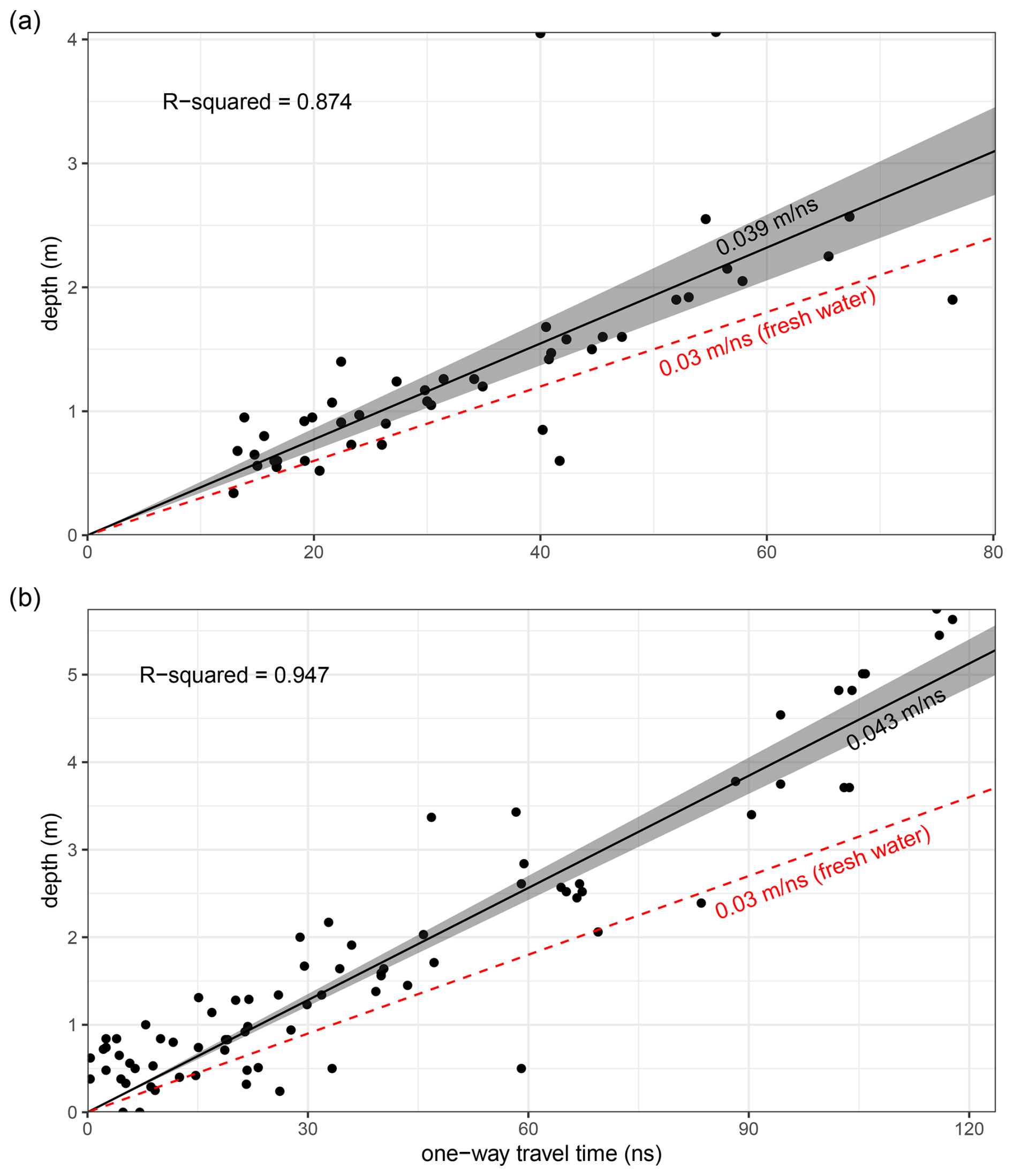
Figure B1 Calibration of GPR wave velocity at Skrimfjella (a) and Ørskogfjellet (b) by regression of probed depth against wave travel time.

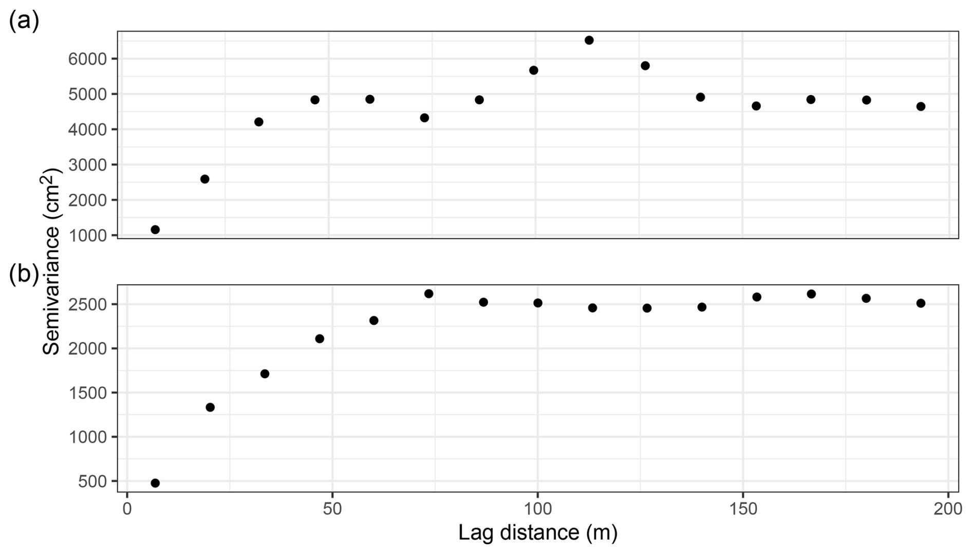
Figure B2 Empirical semivariograms of peat depth point measurements at Skrimfjella (a) and Ørskogfjellet (b).

Appendix C

Table C1 Pairwise comparisons of the concordance correlation coefficient among models for Skrimfjella, based on 10-fold cross-validation. The comparisons use estimated marginal means with Tukey HSD correction and Kenward–Roger degrees of freedom approximation (emmeans package, v.1.11.1; Lenth et al., 2025 ) on mixed-effects models (lme4 package, v.1.1-36; Bates et al., 2015) to account for the cross-validation fold structure.

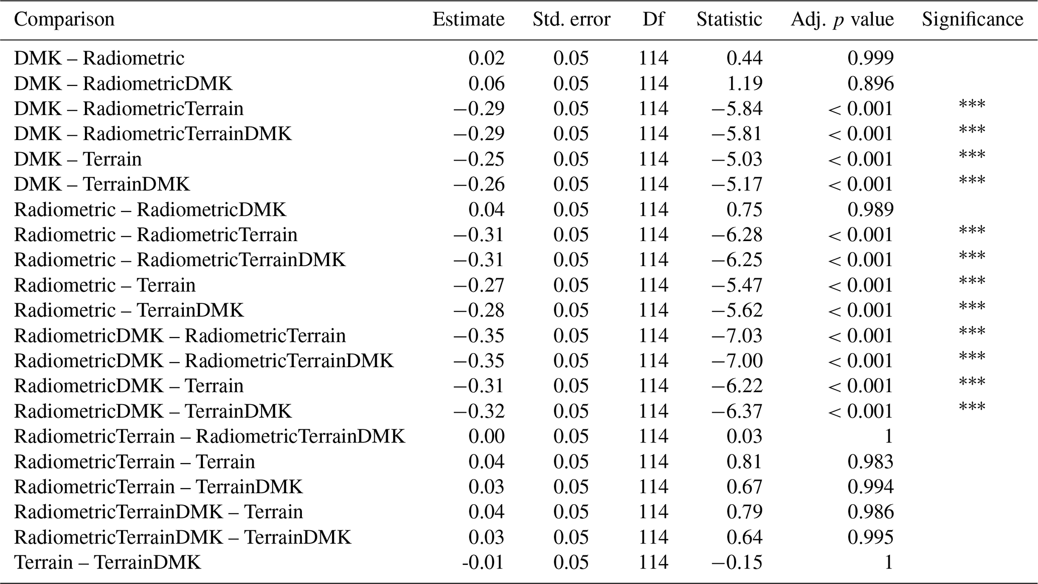
Table C2 Pairwise comparisons of R² among models for Skrimfjella, based on 10-fold cross-validation. The comparisons use estimated marginal means with Tukey HSD correction and Kenward–Roger degrees of freedom approximation (emmeans package, v.1.11.1; Lenth et al., 2025) on mixed-effects models (lme4 package, v.1.1-36; Bates et al., 2015) to account for the cross-validation fold structure.

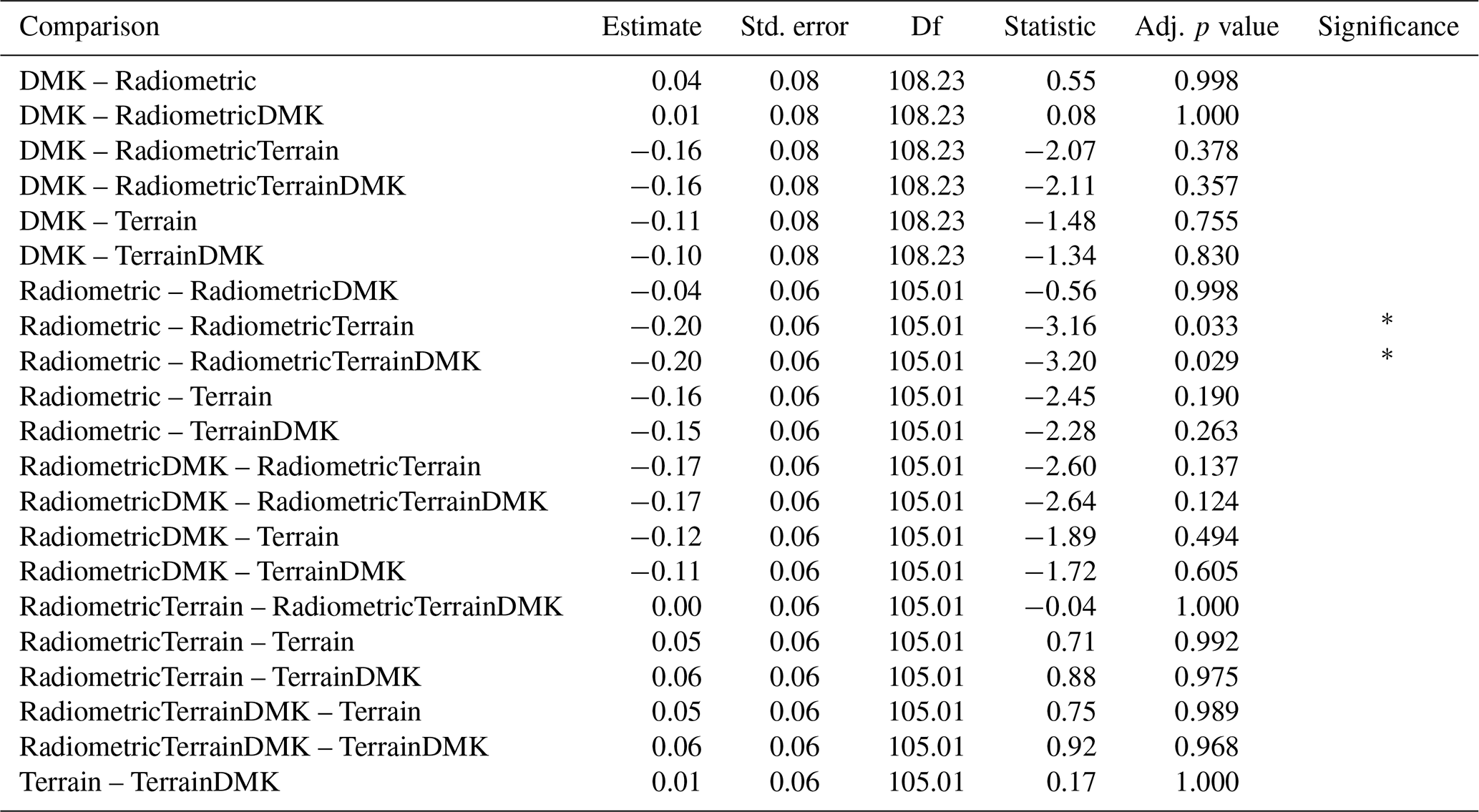
Table C3 Pairwise comparisons of mean absolute error among models for Skrimfjella, based on 10-fold cross-validation. The comparisons use estimated marginal means with Tukey HSD correction and Kenward–Roger degrees of freedom approximation (emmeans package, v.1.11.1; Lenth et al., 2025) on mixed-effects models (lme4 package, v.1.1-36; Bates et al., 2015) to account for the cross-validation fold structure.

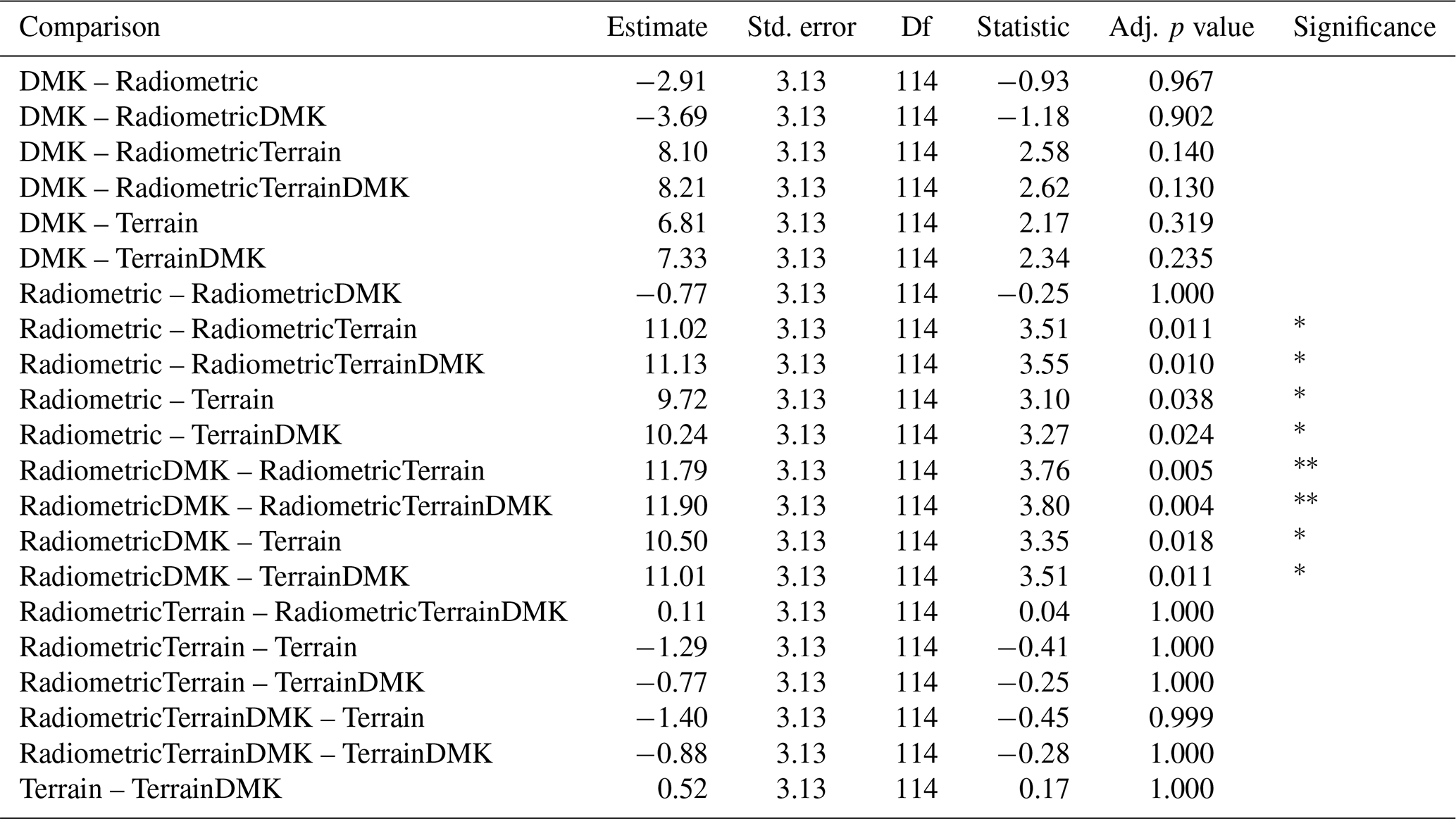
Table C4 Pairwise comparisons of the concordance correlation coefficient among models for Ørskogfjellet, based on 10-fold cross-validation. The comparisons use estimated marginal means with Tukey HSD correction and Kenward–Roger degrees of freedom approximation (emmeans package, v.1.11.1; Lenth et al., 2025) on mixed-effects models (lme4 package, v.1.1-36; Bates et al., 2015) to account for the cross-validation fold structure.

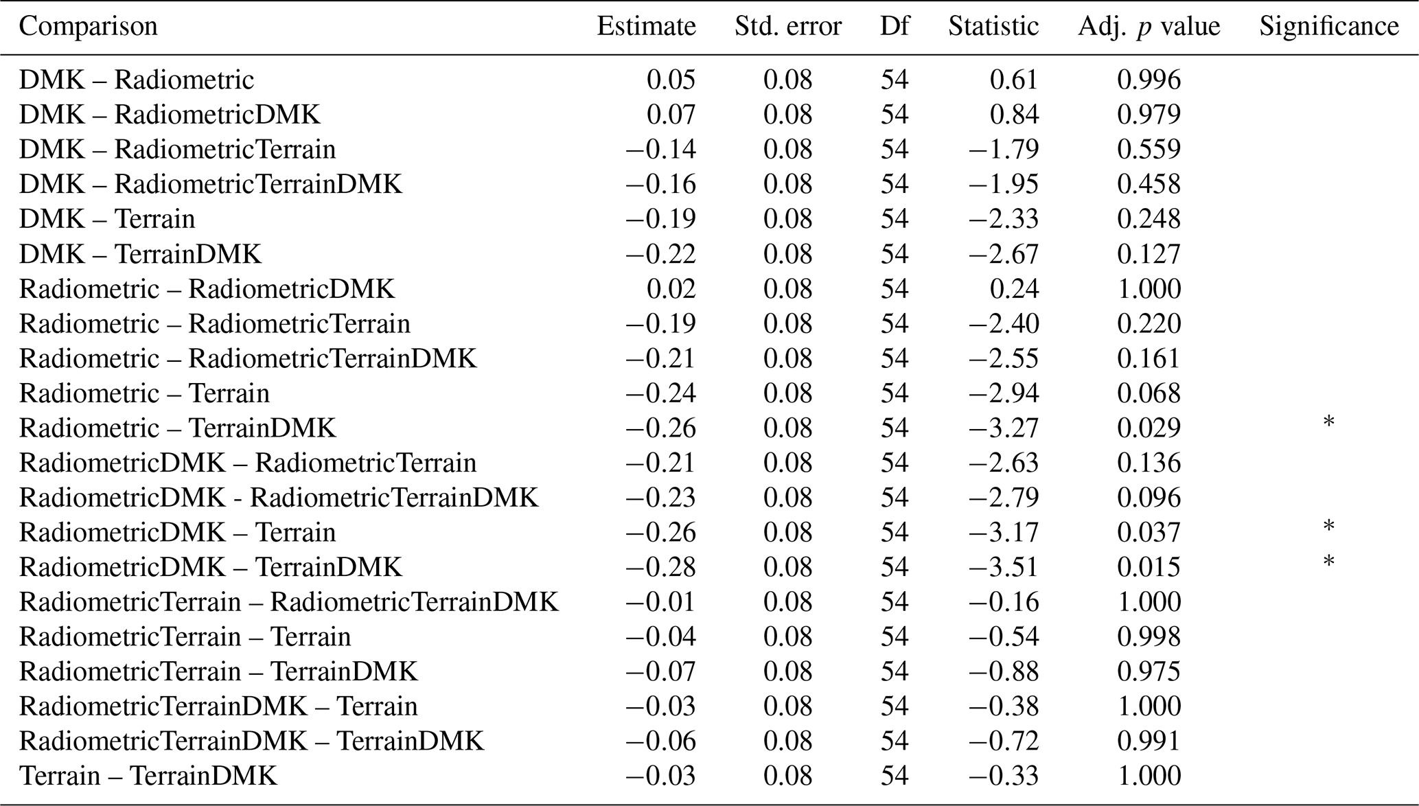
Table C5 Pairwise comparisons of R² among models for Ørskogfjellet, based on 10-fold cross-validation. The comparisons use estimated marginal means with Tukey HSD correction and Kenward–Roger degrees of freedom approximation (emmeans package, v.1.11.1; Lenth et al., 2025) on mixed-effects models (lme4 package, v.1.1-36; Bates et al., 2015) to account for the cross-validation fold structure.

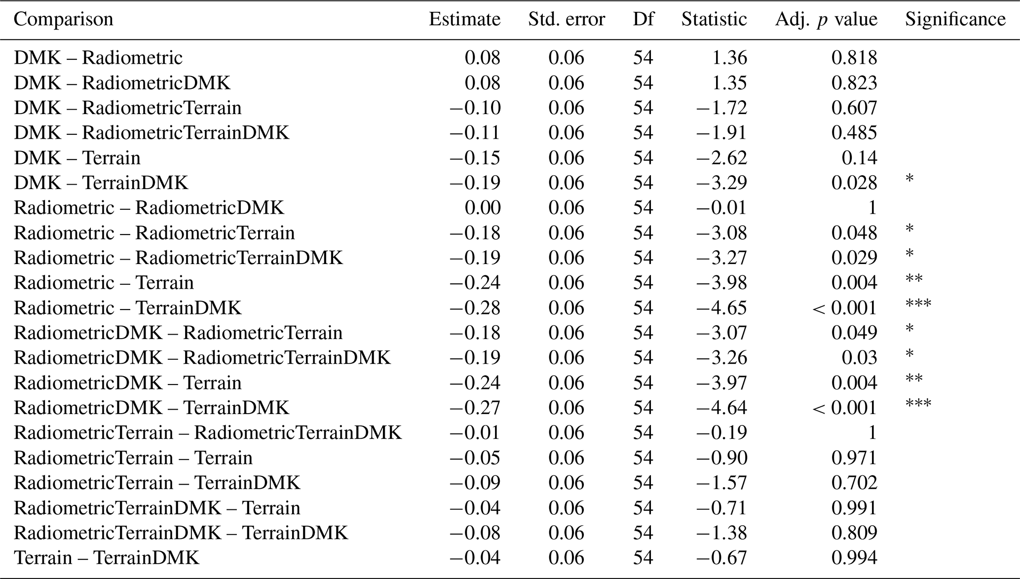
Table C6 Pairwise comparisons of mean absolute error among models for Ørskogfjellet, based on 10-fold cross-validation. The comparisons use estimated marginal means with Tukey HSD correction and Kenward–Roger degrees of freedom approximation (emmeans package; Lenth et al., 2025) on mixed-effects models (lme4 package; Bates et al., 2015) to account for the cross-validation fold structure.