Quantifying hydrological impacts of compacted sandy subsoils using soil water flow simulations: the importance of vegetation parameterization

Numerical models can quantify subsoil compaction's hydrological impacts, useful to evaluate water management measures for climate change adaptations on compacted subsoils (e.g., augmenting groundwater recharge). Compaction also affects vegetation growth, which, however, is often parameterized using only limited field measurements or relations with other variables. This study shows that uncertainties in vegetation parameters linked to transpiration (leaf area index [LAI]) and water uptake (root depth distribution) can significantly affect hydrological modeling outcomes. The HYDRUS-1D soil water flow model was used to simulate the soil water balance of experimental grass plots on Belgian Campine Region's sandy soil. The compacted plot has the compact subsoil at 40–55 cm depths while the non-compacted plot underwent de-compaction. Using two year soil moisture sensor data at two depths, these models of these compacted and non-compacted plots were calibrated and validated under three different vegetation parameterizations, reflecting various canopy and root growth reactions to compaction. Water balances were then simulated under future climate scenarios.

The experiments reveal that the compacted plots exhibited lower LAI while the non-compacted plots had deeper roots. Considering these vegetations' reactions in models, model simulations show that compaction will not always reduce deep percolation, compensated by the deep rooted non-compacted case model's higher evapotranspiration. Therefore, this affected vegetation growth can also further influence the water balance. Hence, hydrological modeling studies on (de-)compaction should dynamically incorporate vegetation growth above- and belowground, of which field evidence is vital.

1 Introduction

Soil compaction has been a persistent worldwide issue that has reduced agricultural yields (Ishaq et al., 2001; Saqib et al., 2004) and even forest growth rates (Nawaz et al., 2013). It comprises at least 17 % of anthropogenic soil degradation cases in Europe and 4 % worldwide (Alakukku, 2012; Oldeman et al., 1991). It occurs when soils are subjected to stresses exceeding their strength (Dexter, 1988). The sources of soil stresses could be natural (e.g., drying/freezing, rainfall, roots, soil mineralogy and parent material, higher clay content present, foot traffic, animal grazing) or artificial (e.g., machinery) (Houšková and Montanarella, 2008; Nawaz et al., 2013; Shaheb et al., 2021; Yang et al., 2022; Zhao et al., 2007). These stresses lead to increased soil bulk densities and reduced porosities and infiltration rates (Nawaz et al., 2013; Silva et al., 2008; Soil Science Society of America, 2008). In turn, these changes in physical parameters can stunt plant growth in terms of height, biomass, roots (depth, length, penetration), and leaf growth (leaf area) (Gliński and Lipiec, 2018; Kristoffersen and Riley, 2005; Nawaz et al., 2013; Passioura, 2002; Shah et al., 2017; Shaheb et al., 2021). Compaction is more persistent in subsoils than topsoils because the natural alleviating processes (wetting/drying, freezing/thawing, root growth) rapidly diminish with depth (van den Akker and Schjønning, 2003; Batey, 2009).

Compaction also affects soil hydrological processes. Topsoil compaction promotes surface runoff especially during heavy precipitation events because of hindered vertical infiltration by reduced macropore volumes (Alaoui et al., 2018; Byrd et al., 2002). Moreover, it also promotes evaporation due to the small pores that favor more capillary flow (Goldberg-Yehuda et al., 2022; Romero-Ruiz et al., 2022). For subsoils, compact layers (such as plow or tillage pans) have a higher bulk density and a lower total porosity (smaller and more isolated pores) than the soil directly above or below it (Bertolino et al., 2010; Gliński et al., 2011). This then prevents surplus water from further percolating (Adekalu et al., 2006; Allmaras, 2003; Bertolino et al., 2010), thereby increasing soil moisture on the zones above the dense layer (Moreno et al., 2003; Nawaz et al., 2013) and lateral flow above the plow pan (interflow) and runoff (Alaoui et al., 2018; Jiang et al., 2015). With more retained soil moisture, more water is available for evaporation (Agrawal, 1991; Assaeed et al., 1990; Hoefer and Hartge, 2010) and root water uptake (and thus transpiration). However, the stunted root growth brought by compaction reduces soil water uptake in the dense subsoil and deeper zones (Bengough et al., 2011; Passioura, 2002; Wang et al., 2019). This is then compensated by increased uptake in looser soils overlying the dense subsoil, attributed mainly to increased soil-root contact and higher unsaturated hydraulic conductivity promoting more water flow (Andersen et al., 2013; Lipiec and Hatano, 2003; Nosalewicz and Lipiec, 2014). Moreover, stunted leaf growth, manifested by reduced leaf areas, hindered transpiration (Assaeed et al., 1990; Grzesiak, 2009; Umaru et al., 2021). Subsoil compaction also hinders deeper percolation and hence groundwater recharge (Negev et al., 2020; Owuor et al., 2016; Radatz et al., 2012). De-compaction is thus recommended to promote recharge (Garcia and Galang, 2021; Priori et al., 2020; Tarigan et al., 2020). In short, subsoil compaction leads to higher accumulated soil moisture above the compact subsoil layer, higher runoff, and lower deep percolation, but transpiration and evaporation can be higher or lower with compaction (Appendix A – Fig. A1, Appendix B – Table B1).

These conclusions from experimental observations were further confirmed by hydrological modeling studies that quantify compaction's impacts on soil water fluxes. These models are also useful to simulate hydrological impacts that can guide water resource management under climate change scenarios. However, accurate model simulations require accurate estimates of model parameters that should be based on accurate measurements (Moreno et al., 2003). Given that transpiration has a large impact on the soil water, vegetation parameters related to root water uptake and leaf area are thus important. Therefore, the impact of soil compaction on vegetation parameters should also be included in model simulations to assess the overall effect on soil water fluxes. However, vegetation parameter values were mostly based on limited field measurements (i.e., taken only at the end of harvesting period), assumptions based on correlations or derivations from other variables, or calibrations/parameter estimations. Some of these parameters were even assumed to be the same for compacted and non-compacted setups (Appendix B – Table B1), examples of which are leaf area indices (LAI) (Moreno et al., 2003; Voter and Loheide, 2018) and root development (Hartmann et al., 2012; Romero-Ruiz et al., 2022).

These modeling studies also focused mostly on fine soil textures (i.e., silty, loamy). Only one hydrological modeling study on compaction involved sandy soils (Moreno et al., 2003) (Appendix B – Table B1), which reported negligible hydrological impacts of compaction. But, sandy subsoils exhibit higher susceptibility to machinery-induced compaction than loam or clay subsoils (Jones et al., 2003; Scanlan et al., 2022; Spoor et al., 2003). Moreover, sandy soils are globally relevant, occupying 31 % of total global area comprising all continents (De Holanda et al., 2023; Huang and Hartemink, 2020).

Hence, for these less studied sandy soils, this paper shows how such uncertainties in vegetation parameters related to transpiration and root water uptake can largely affect the modeling outcomes. Here, pilot experiments involving vegetated plots with intact compact sandy subsoil and plots which underwent de-compaction were performed. Calibrated and validated 1D soil water flow models (HYDRUS), parameterized based on these experiments, were used to disentangle these plots' water budgets under various climate scenarios.

2 Materials and Methods

2.1 Experimental Site and Setup

The study site is located southeast of Lille, Province of Antwerp, northern Belgium (Appendix A – Fig. A2) within the Kleine Nete watershed of the Campine Region. The site elevation is about 10 m above sea level. The land use near the site is grassland and arable land (maize and potatoes are the main crops) and the site has been under grasslands since 1970s. The site has a temperate oceanic climate (Peel et al., 2007). Over the years 1979–2023, annual precipitation and potential evapotranspiration values range from 480–890 and 500–800 mm respectively (Toreti, 2014).

The site's soil is loamy sand with anthropogenic humus A horizon (Bogemans, 2005). A compacted subsoil at 40 to 55–60 cm depth is present, which is an iron oxide pan (Bsm horizon) having green color and red-orange concretions (Appendix A – Fig. A3). This pan is also reported to be common on sandy soils found east of Antwerp, Belgium (Vandamme, 1978), where the study site is situated. Other soil types within the site's vicinity are in Appendix A – Fig. A4.

Eight 2 m square plots were constructed at the site in December 2021. Four of them were de-compacted by excavating the soil down to 150 cm depth using a crane to eliminate the compact layer (Appendix A – Figs. A5, A6). To check the effectiveness of de-compaction, penetrometer logs were also used wherein the lack of peaks in pressure values indicate the absence of compacted layer (Fig. 2a). The remaining four plots still have the compact layer intact (Fig. 2b, Appendix A – Fig. A5).

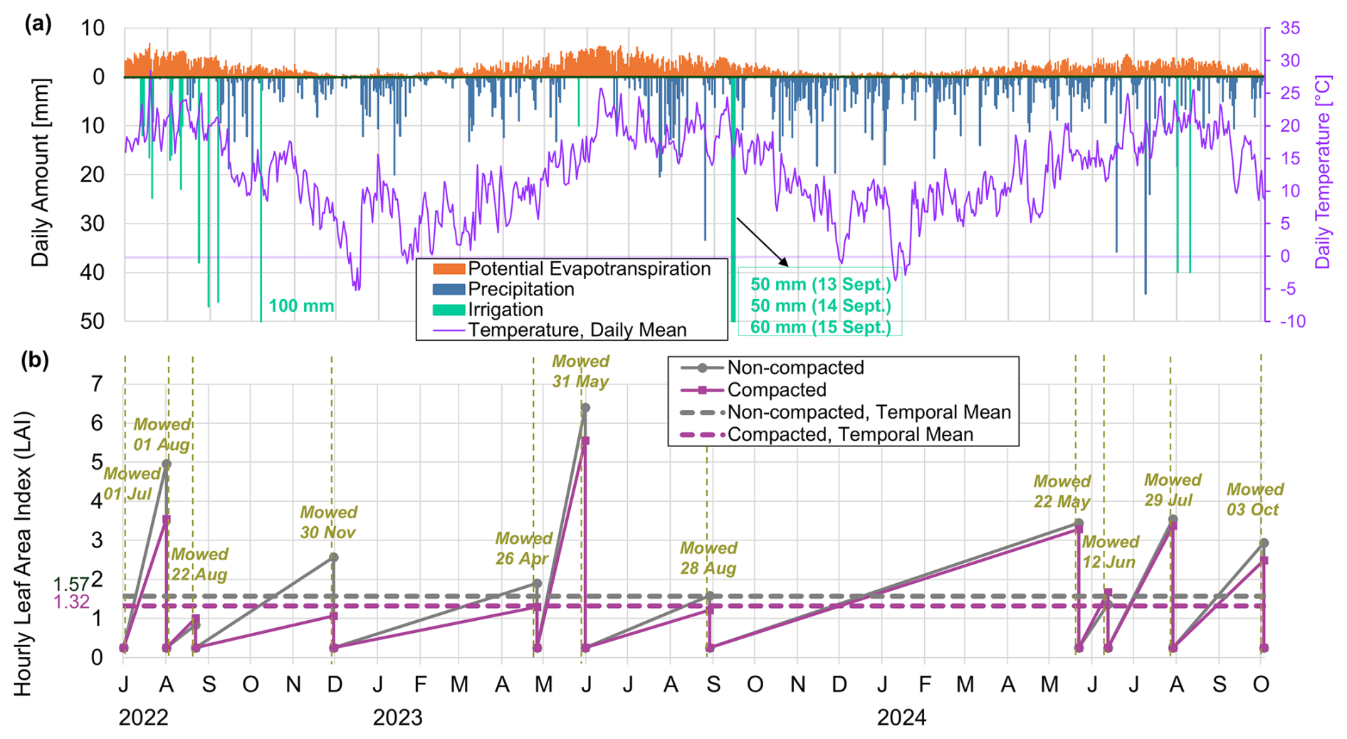
Figure 1 Daily time series of (a) potential evapotranspiration, precipitation, mean temperatures, and applied irrigation amounts during the experiments, (b) leaf area index (LAI) for grass-clover mixtures under non-compacted and compacted cases and mowing timeline.

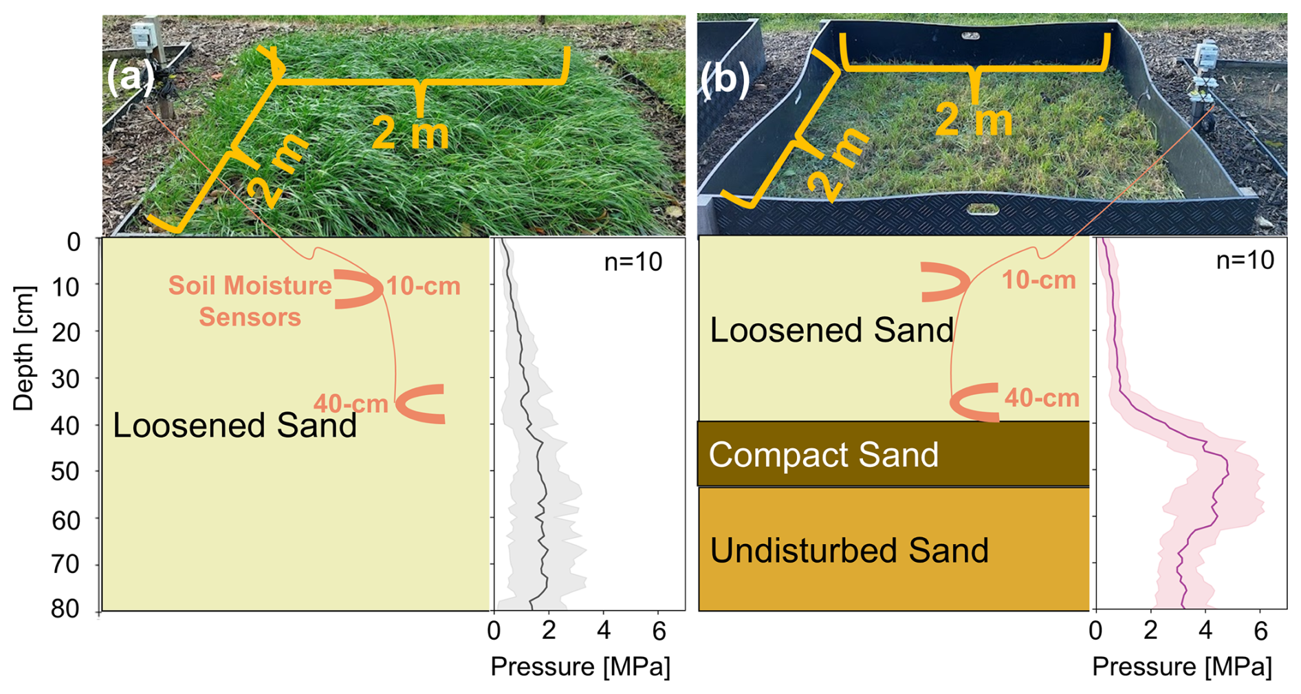
Figure 2 Experimental plots, schematic soil profiles, and averaged penetrologger profiles (± standard deviation, represented by shaded bands) for (a) a non-compacted case and (b) a compacted case.

For each plot, the excavated sandy topsoil layer (40 cm thick for compacted plots and 150 cm thick for non-compacted plots, Fig. 2) was loosened and homogenized well using a cement mixer and then returned to that same plot. In four plots, 480 L woodchips were also mixed, mimicking Campine Region's general agricultural practice (Appendix A – Fig. A5). Impermeable plastic boxes were installed to avoid subsurface lateral in or outflow (Appendix A – Fig. A6). Per plot, two capacitance sensors (HOBO Onset S-SMC-M005) monitored the soil moisture content at 10 and 40 cm depths, allowing to capture the hydrological conditions near the surface and right above the compact subsoil layer, respectively (Fig. 2). This monitoring spanned from 8 July 2022 to 8 September 2024.

Each plot had either maize (Zea mays) or mixtures of Italian ryegrass (Lolium multiflorum) and white clover (Trifolium repens) as vegetation cover (Appendix A – Fig. A5), thus replicating Campine Region's general agricultural landscape. No plots were fertilized.

The grass-clover mixtures were mowed to 15 cm stubble height (mowing timeline in Fig. 1b and Appendix A – Fig. A7) whenever they appeared to grow beyond the plot boxes (Fig. 2). As shown in Eq. (1), the clippings' dry weights were converted into LAI using a representative leaf dry mass of 66 g m⁻², based on the mean of the median leaf dry mass of herbs (60 g m⁻², representing white clover) and of graminoids (72 g m⁻², representing grass) (Poorter et al., 2009)

$$\begin{array}{}\text{(1)}& \mathrm{LAI}={\displaystyle \frac{\left(\frac{\text{dried weights of grass-clover mixture}}{\text{mean leaf dry mass per unit leaf area}}\right)}{\text{plot area}}}\end{array}$$

Temporal hourly LAI values during grass-clover's growths (Fig. 1b) were linearly interpolated from the LAI after last mowing and LAI before the next mowing. The LAI after last mowing, pertaining to the grass remaining after mowing, was always assumed to be 0.25, significantly lower than the lowest LAI from clippings (0.84–1.01) (Fig. 1b). This LAI after the last mowing was then added with LAI from the next mowing's weighed clippings to obtain the overall LAI before last mowing.

Maize was sown on 26 April 2022; 11 May 2023; and 22 May 2024 and then harvested on the onset of wet season on 17 October 2022; 20 October 2023; and 8 October 2024. Harvesting was done by cutting them down, leaving 10 cm stem above ground level, whereafter the maize plots were left fallow.

Outside the plots, eight non-compacted sand and seven compact sand samples were obtained at 15 and 50 cm depths, respectively. Their grain size compositions were estimated by laser diffraction technique. Their bulk densities were estimated based on their dry masses and ring kit volumes. Saturated hydraulic conductivity (K_s) was estimated from the falling head method (Table 1).

Table 1 Laboratory measurements of soil properties. Values in parenthesis denote the geometric mean for K_s and arithmetic mean for the rest.

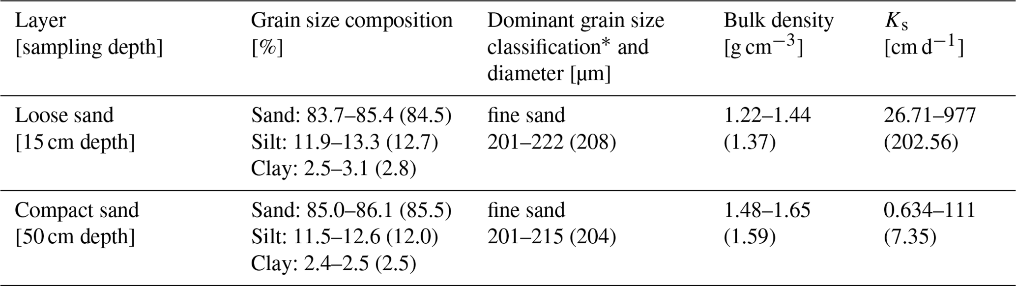
^* Based on Harmonized world soil database version 2.0 (FAO and IIASA, 2023).

Precipitation, air temperature (Fig. 1a), solar radiation, relative humidity, and average wind velocity were measured on an hourly resolution using a local weather station located 2 km from the site. Measurement gaps were filled using the data from the closest active meteorological station at Herentals (Flemish Environment Agency, 2021), 5.5 km away from the site. Daily mean temperature ranged from −5.2 °C (in December 2022) to 27.5 °C (in July 2022) during the experiments (Fig. 1a). From these meteorological variables, the potential evapotranspiration (ET₀) [mm h⁻¹] was derived using the Food and Agriculture Organization (FAO) 56 Penman-Monteith Equation for a reference crop (hypothetical grass surface) (Allen et al., 1998), shown in Eq. (2).

$$\begin{array}{}\text{(2)}& \begin{array}{rl}& {\mathrm{ET}}_{\mathrm{0}}={\displaystyle \frac{\mathrm{0.408}\mathrm{\Delta }\left(R_{\mathrm{n}}-G\right)+\mathit{\gamma }{U}_{\mathrm{2}}(e_s-e_a)\left(\frac{\mathrm{37}}{T+\mathrm{273}}\right)}{\mathrm{\Delta }+\mathit{\gamma }(\mathrm{1}+\mathrm{0.34}{U}_{\mathrm{2}})}}\\ & G=\mathrm{0.1}{R}_{\mathrm{n}},R_{\mathrm{n}}>\mathrm{0}\text{[daytime] }\\ & G=\mathrm{0.5}{R}_{\mathrm{n}},R_{\mathrm{n}}\le \mathrm{0}\text{[nighttime] }\end{array}\end{array}$$

where Δ is the slope of the vapor pressure curve [kPa °C⁻¹], R_n is the net radiation at the grass' surface [MJ m⁻² h⁻¹], G is the soil heat flux [MJ m⁻² h⁻¹] whose calculation depends on the sign of R_n that indicates if the hourly R_n was measured at daytime or nighttime, γ is the psychrometric constant [kPa °C⁻¹], U₂ is the wind speed measured at 2 m height [cm s⁻¹], e_s−e_a is the vapor pressure deficit [kPa] and T is the average air temperature [°C]. The resulting daily potential evapotranspiration and comparison with precipitation are shown in Fig. 1a.

In 2022, intense summer rainfall events that could generate surface runoff and could be more frequent in the future climate (Hodnebrog et al., 2019; Hosseinzadehtalaei et al., 2020) were mimicked by irrigating the plots. Irrigation is performed by sprinkling using 10 L graduated watering cans. Applied irrigation doses are listed and justified in Appendix B – Tables B2 and B3.

At the end of the monitoring period, the roots inside plots with grass-clover mixtures were sampled. For each of these plots, a root length density profile and a dry biomass profile were obtained. Root-soil cores (8 cm diameter, 15 cm height) were extracted every 15 cm throughout the 0–105 cm depths using root augers. These cores were then washed thoroughly to obtain the roots. The root lengths were estimated using the grid-intersection method and Eq. (3) (Freschet et al., 2021; Newman, 1966; Tennant, 1975). These roots were also oven-dried at 70 °C for a week and then weighed.

$$\begin{array}{}\text{(3)}& \begin{array}{rl}& \text{Root length}=\\ & {\displaystyle \frac{\mathrm{11}}{\mathrm{14}}}\times \text{total number of intercepts}\left(\text{horizontal and vertical}\right)\\ & \times \text{grid unit length}\end{array}\end{array}$$

The timeline of these experiments is summarized in Appendix A – Fig. A7.

2.2 Numerical Model Setup

The experimental plots were represented as 1D soil columns, assuming that lateral flow there was insignificant (Fig. 2). The soil water hydrology was modeled using the numerical model HYDRUS-1D (Šimůnek et al., 2008).

2.2.1 Soil Water Movement

The HYDRUS-1D code simulates 1D (vertical) water movement in porous media by numerically solving the Richards equation for water flow along variable-saturated media, neglecting air phase and thermal gradient-driven flow (Richards, 1931; Šimůnek et al., 2008), shown in Eq. (4).

$$\begin{array}{}\text{(4)}& {\displaystyle \frac{\partial \mathit{\theta }}{\partial t}}={\displaystyle \frac{\partial }{\partial z}}\left[K\left(h\right)\left({\displaystyle \frac{\partial h}{\partial z}}+\mathrm{1}\right)\right]-S\left(h\right)\end{array}$$

where h is the water pressure head [L], θ is the soil moisture content (SMC) [L³ L⁻³], t is time [T], z is the spatial coordinate [L], S(h) is the sink term [L³ L⁻³ T⁻¹] that accounts for root water uptake and K(h) is the unsaturated hydraulic conductivity function [L T⁻¹].

The van Genuchten-Mualem functions were used to describe the θ(h) and K(h) relations (Mualem, 1976; Van Genuchten, 1980), shown in Eq. (5):

$$\mathit{\theta }\left(h\right)=\left\{\begin{array}{ll}{\mathit{\theta }}_{\mathrm{r}}+\frac{{\mathit{\theta }}_{\mathrm{s}}-{\mathit{\theta }}_{\mathrm{r}}}{{\left[\mathrm{1}+{\left|\mathit{\alpha }h\right|}^n\right]}^m}& h<\mathrm{0}\\ {\mathit{\theta }}_{\mathrm{s}}& h\ge \mathrm{0}\end{array}\right.$$

$$\begin{array}{}\text{(5)}& K\left(h\right)=K_{\mathrm{s}}{S}_{\mathrm{e}}^L{\left[\mathrm{1}-{\left(\mathrm{1}-S_{\mathrm{e}}^{-\mathrm{1}/m}\right)}^m\right]}^{\mathrm{2}}\end{array}$$

$$\begin{array}{c}{\displaystyle }{S}_{\mathrm{e}}={\displaystyle \frac{\mathit{\theta }-{\mathit{\theta }}_{\mathrm{r}}}{{\mathit{\theta }}_{\mathrm{s}}-{\mathit{\theta }}_{\mathrm{r}}}}\\ {\displaystyle }m=\mathrm{1}-{\displaystyle \frac{\mathrm{1}}{n}},n>\mathrm{1}\end{array}$$

where the θ_s and θ_r are the saturated and residual soil water content, respectively. K_s is the saturated hydraulic conductivity [L T⁻¹]. S_e is the effective water content. α [L⁻¹] and n [–] are empirical parameters of the water retention curve functions. Together with the tortuosity and pore connectivity parameter L, these empirical parameters influence the hydraulic functions' shape. In the model setups, L was set to 0.5, the value frequently applied for mineral soils (Dettmann et al., 2014; Mualem, 1976). The Richards equation is then solved numerically at each node using Galerkin-type linear finite element schemes.

For the root water uptake, the water volume removed from a unit soil volume per unit time (sink term, S) is defined using Eq. (6) (Feddes et al., 1978; Šimůnek et al., 2008)

$$\begin{array}{}\text{(6)}& S\left(h\right)=\mathit{\alpha }\left(h\right)S_{\mathrm{P}}\end{array}$$

where the α(h) [–] is a prescribed function of the soil water pressure head ($\mathrm{0}\le \mathit{\alpha }\le \mathrm{1}$) and S_P [T⁻¹] is the potential water uptake. S_P is further defined using Eq. (7):

$$\begin{array}{}\text{(7)}& S_{\mathrm{P}}=T_{\mathrm{P}}b\left(z\right)\end{array}$$

where T_P is the potential transpiration rate [L T⁻¹], and b(z) is the normalized water uptake distribution [L⁻¹], which reflects S_P's spatial variation throughout the root zone. The b(z) is based on normalized root distributions (b^′(z)) as shown in Eq. (8) (Šimůnek et al., 2008):

$$\begin{array}{}\text{(8)}& b\left(z\right)={\displaystyle \frac{b^{\prime }\left(z\right)}{{\int }_{L_{\mathrm{R}}}{b}^{\prime }\left(z\right)\mathrm{d}z}}\end{array}$$

$$\underset{L_{\mathrm{R}}}{\int }b\left(z\right)\mathrm{d}z=\mathrm{1}$$

where L_R is the root zone region or domain. Solving for T_P by combining Eqs. (7) and (8) leads to Eq. (9):

$$\begin{array}{}\text{(9)}& T_{\mathrm{P}}=\underset{L_{\mathrm{R}}}{\int }{S}_{\mathrm{P}}\mathrm{d}z\end{array}$$

Meanwhile, the actual root water uptake can involve water uptake compensation along root zones. The presence of this compensation depends on the dimensionless water stress index ω, defined in Eq. (10), and a user-defined threshold ω_c (also known as the critical water stress index or root adaptability factor) (Jarvis, 1989; Šimůnek et al., 2008).

$$\begin{array}{}\text{(10)}& \mathit{\omega }=\underset{L_{\mathrm{R}}}{\int }\mathit{\alpha }\left(h,z\right)b\left(z\right)\mathrm{d}z\end{array}$$

When ω exceeds ω_c, reduced root water uptakes in stressed zones within L_R are compensated by other zones' increased uptakes. Otherwise, no compensation occurs. Following Eq. (11), ω_c<1 promotes compensation (fully at ω_c=0) while ω_c=1 inactivates it (Šimůnek et al., 2008).

$$\begin{array}{}\text{(11)}& S(h,z)=\left\{\begin{array}{ll}\mathit{\alpha }(h,z)b\left(z\right)\frac{T_{\mathrm{P}}}{{\mathit{\omega }}_{\mathrm{c}}}& \mathit{\omega }<{\mathit{\omega }}_{\mathrm{c}}\\ \mathit{\alpha }(h,z)b\left(z\right)\frac{T_{\mathrm{P}}}{\mathit{\omega }}& {\mathit{\omega }}_{\mathrm{c}}<\mathit{\omega }<\mathrm{1}\end{array}\right.\end{array}$$

$${\displaystyle \frac{T_{\mathrm{a}}}{T_{\mathrm{P}}}}=\left\{\begin{array}{ll}\frac{{\int }_{L_{\mathrm{R}}}\mathit{\alpha }(h,z)b\left(z\right)\mathrm{d}z}{{\mathit{\omega }}_{\mathrm{c}}}=\frac{\mathit{\omega }}{{\mathit{\omega }}_{\mathrm{c}}}<\mathrm{1}& \mathit{\omega }<{\mathit{\omega }}_{\mathrm{c}}\\ \frac{{\int }_{L_{\mathrm{R}}}\mathit{\alpha }(h,z)b\left(z\right)\mathrm{d}z}{\mathit{\omega }}=\frac{\mathit{\omega }}{\mathit{\omega }}=\mathrm{1}& {\mathit{\omega }}_{\mathrm{c}}<\mathit{\omega }<\mathrm{1}\end{array}\right.$$

where T_a is the actual transpiration rate [L T⁻¹].

2.2.2 Boundary Conditions

The upper boundary condition (atmospheric boundary condition with surface runoff) (Fig. 3) involved meteorological forcings related to precipitation and potential evapotranspiration. For precipitation, the hourly values recorded by the site's weather station were used. For potential evapotranspiration, the hourly values (ET₀) were calculated using Eq. (2) and then partitioned to potential transpiration (T_P) and potential soil evaporation (E_P) in HYDRUS based on LAI in accordance to the Beer's Law, shown in Eq. (12) (Ritchie, 1972; Šimůnek et al., 2008).

$$T_{\mathrm{P}}={\mathrm{ET}}_{\mathrm{0}}\times \left(\mathrm{1}-e^{-\mathrm{rExtinct}\left(\mathrm{LAI}\right)}\right)$$

$$\begin{array}{}\text{(12)}& E_{\mathrm{P}}={\mathrm{ET}}_{\mathrm{0}}-T_{\mathrm{P}}={\mathrm{ET}}_{\mathrm{0}}\times e^{-\mathrm{rExtinct}\left(\mathrm{LAI}\right)}\end{array}$$

where rExtinct is the radiation extinction coefficient, equal to 0.463 (Šimůnek et al., 2008). The LAI time series for non-compacted or compacted plots (Fig. 1b) was used to parameterize the corresponding case's ET₀ partitioning.

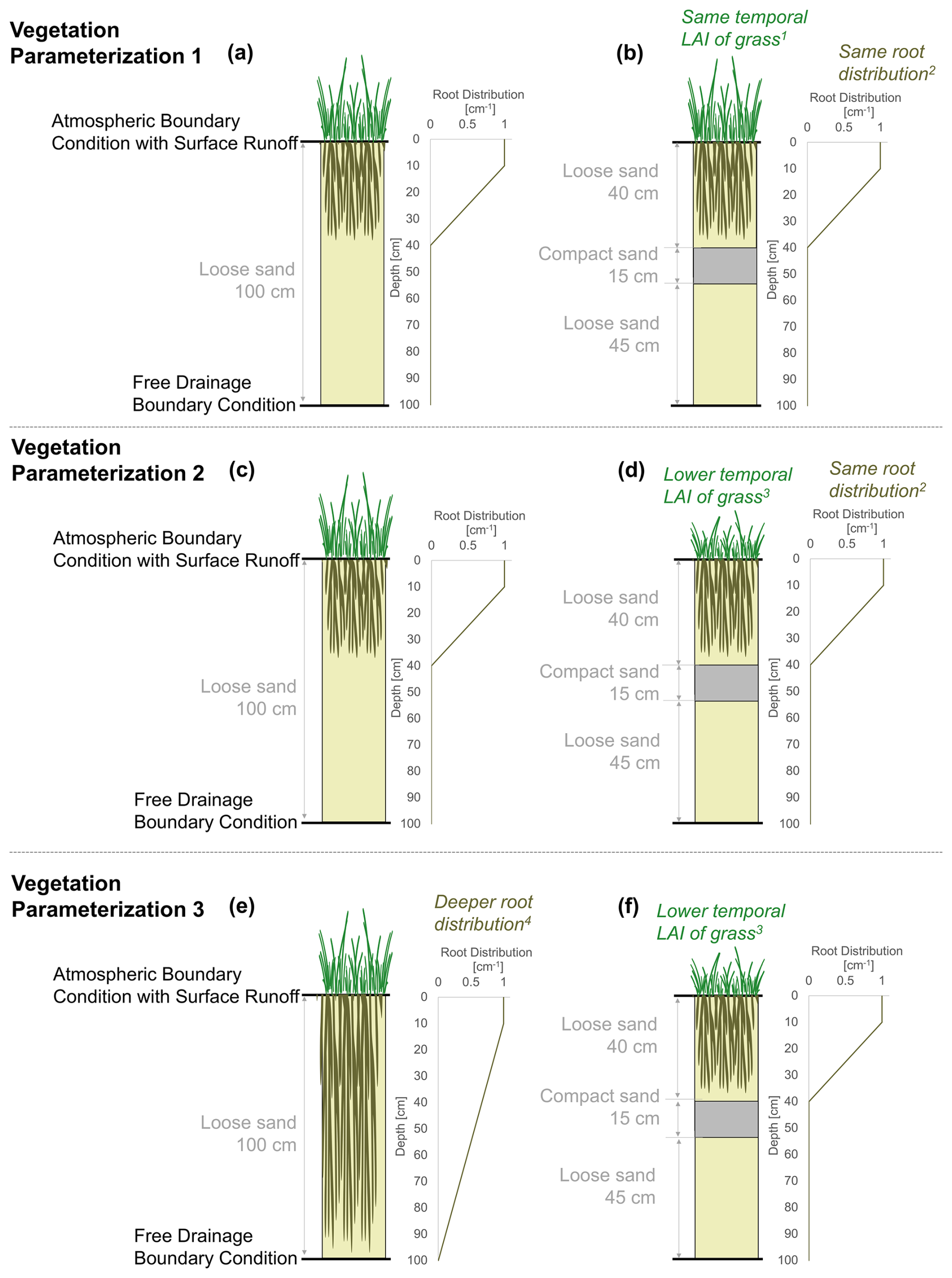
Figure 3 Schematic diagram of 1D soil water flow models for non-compacted and compacted cases under the three vegetation parameterizations. ¹ Leaf Area Index (LAI) adopted only from the non-compacted case in the experimental plots (Fig. 1b). ² Rooting depth reaches to 40 cm and distribution is 1 from 0–10 cm depths and linearly decreasing to 0 from 10 to 40 cm depths. ³ LAI adopted from non-compacted and compacted cases in the experimental plots, respectively (Fig. 1b). ⁴ Non-compacted case model: distribution is 1 (0–10 cm depths), then linearly decreasing to 0 (10 to 100 cm depths); compacted case: distribution is 1 from 0–10 cm depths and linearly decreasing to 0 from 10 to 40 cm depths.

Runoff was calculated whenever the pressure head reached zero at the soil surface. Ponding was disregarded to simplify the quantification of this excess water in the simulations.

The lower boundary condition was set to free drainage (zero gradient boundary condition; Šimůnek et al., 2008) (Fig. 3). This is based on the water table being significantly deeper (200 cm) than the compact layer's bottom depth (55–60 cm) as observed from the soil profiles from March 2023 and March 2024. Even when considering capillary rise (+13.5 to +50 cm for fine sands; Fetter, 1994), the capillary fringe was likely still deeper than the compact layer.

2.2.3 Vegetation Parameterizations

Grass was considered as the model setups' vegetation. Since the grass had been present throughout the experimental period, root distributions are assumed to be constant in time. Root water uptake compensation (Jarvis, 1989; Šimůnek et al., 2008) was also permitted using ω_c=0.1. This is because the default Feddes model parameter values for grasses in HYDRUS-1D (Feddes et al., 1978; Šimůnek et al., 2008) lead to underestimated root water uptake values for coarse-textured soils (Peters et al., 2017) like the sandy soils in this study. These underestimations are relevant especially when simulating dry and wet water stress conditions.

In setting up the model, three approaches on vegetation parameterizations were considered to examine the impact of varying vegetation parameters (likely affected by compaction) on the soil water balance components. For each vegetation parameterization, two setups (non-compacted and compacted) were represented with the compact layer at 40–55 cm depths. For each model setup, the soil profile ranged from 0–100 cm (Fig. 3), having 211 nodes. The 0–55 cm depth had constant fine spatial resolution of $\mathrm{1}/\mathrm{3}$ cm because this depth involved more relevant hydrologic processes (e.g., soil evaporation, runoff), the observation points at 10 and 40 cm, and an additional compact layer for the compacted case models. The remaining 55–100 cm depths had constant coarser 1 cm resolution to save computational time and power.

In Vegetation Parameterization 1, compaction is assumed to not affect the vegetation, i.e., no effect on LAI and root depth. Since no roots were observed to develop in the compact layer (Appendix A – Fig. A8), the roots were limited to 40 cm depths in both compacted and non-compacted case models (Fig. 3a, b). This is also the typical root biomass distribution of Italian ryegrass in loamy clay Cambisol under a temperate oceanic climate (Durand et al., 2010; Kunrath et al., 2015) and in a loamy soil under phytotron conditions (24 °C at day, 22 °C at night, relative humidity 80 %, 16 h photoperiod) (Lambrechts et al., 2014). The non-compacted plots' LAI time series (Fig. 1b) was adopted for both the compacted and non-compacted case models. With this, transpiration has more weight than soil evaporation even in the compacted case model.

In Vegetation Parameterization 2, the same root distribution was again assumed in the compacted and non-compacted case models. However, the effect of the soil compaction on the LAI was also considered (Fig. 3c, d). Thus, the measured LAI time series was used for each respective case (Fig. 1b). Compared to the previous parameterization, less weight is given to transpiration than evaporation in the compacted case model. Furthermore, this parameterization represents yield decrease in compacted soils, also reported for sandy subsoils (Laker, 2001; Laker and Nortjé, 2020; Pumphrey et al., 1980).

In Vegetation Parameterization 3, both the LAI and root distribution varied between the compacted and non-compacted case models (Fig. 3e, f). The setup was similar to Vegetation Parameterization 2 for the compacted case model. However, a deeper root distribution (i.e., 100 cm depth) was applied for the non-compacted case model (Fig. 3e). These are based on observed larger root length and biomass densities and deeper root depths for the non-compacted plots (Appendix A – Fig. A8). This also represents the vegetation's response to the lower water availability in sandy soils by developing a deeper root zone with more access to deeper soil water especially under drier periods. Meanwhile, the compacted setup's roots cannot penetrate in the subsoil (Harrison et al., 1994; Vanderhasselt et al., 2024). This vegetation parameterization allows to reduce the drought stress and leads to more transpiration in the non-compacted soil than in the previous vegetation parameterizations.

2.2.4 Soil Hydraulic Properties: Model Calibration and Validation

For model calibration, a single soil hydraulic parameter set was selected for all vegetation parameterizations based on HYDRUS-1D's inverse modeling of both non-compacted and compacted cases under Vegetation Parameterization 3. With this, no differences in soil parameters can contribute to the differences between these vegetation parameterizations' results. The period of 8 July 2022 (the start of soil moisture monitoring) until 30 September 2023 was selected for calibration, covering both wet and dry periods. The next hydrological year (1 October 2023 to 8 September 2024) was used for model validation.

The constraints of residual soil water content (θ_r), saturated soil water content (θ_s), α and n (Appendix B – Table B4) were derived from the measured grain size distribution and bulk densities using ROSETTA pedotransfer function (version 2) (Schaap et al., 2004). The constraints for K_s of loose and compact sand layers were based on falling head permeameter tests (Table 1). The hydraulic properties of the loose sand layers in both non-compacted and compacted plots were assumedly the same, given their similar grain size composition (Table 1) and complete homogenization in the field.

The soil moisture time-series used for inverse modeling are averages of observations taken across compacted and de-compacted plots (Appendix A – Fig. A9), regardless of the applied treatments (Appendix A – Fig. A5). The initial soil moisture content values throughout the profiles were based on linear interpolation involving these averaged soil moisture content measurements at 10 and 40 cm depths (corresponding to last hour before the first hour of simulations). Mean soil moisture measurements during hours with below 0 °C air temperatures were discarded as they might not reflect the actual moisture content under freezing conditions.

The loose soil's parameter values were derived first using observations from the non-compacted plots. These obtained values were then adopted and fixed for the compacted case's loose layers so that only the compact subsoil layer's parameters remained to be optimized via inverse modeling using the compacted plots' mean soil moisture time series. The resulting water retention and conductivity curves depicting the estimates from the inverse models and from the ROSETTA functions for field samples are in Appendix A – Figs. A10, A11.

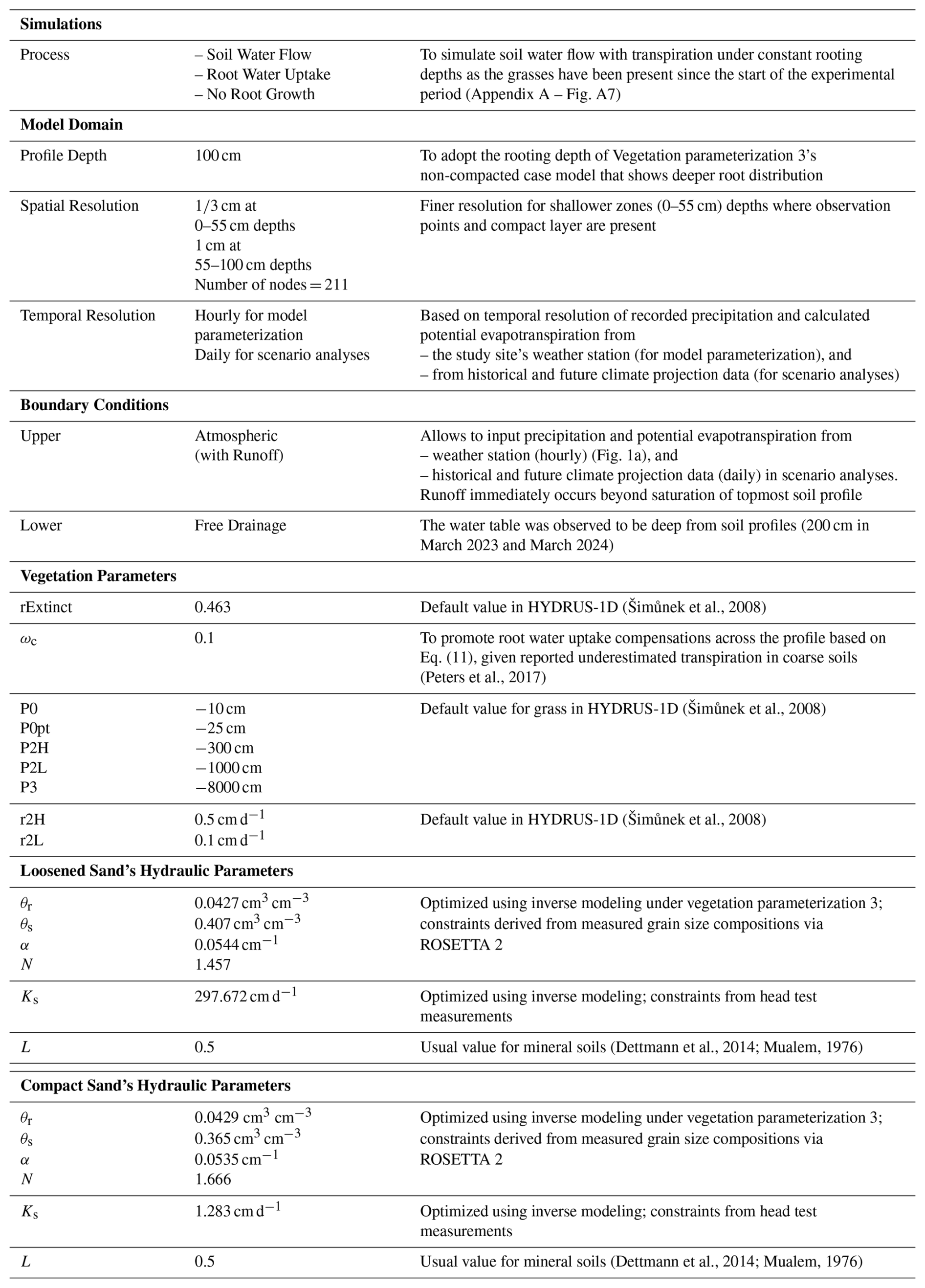
Table 2 summarizes the parameter values and settings used in the non-compacted and compacted case models under all vegetation parameterizations.

Table 2 Model parameter specifics and justifications applied to all vegetation parameterizations.

2.3 Scenario Analyses

The calibrated and validated models were then used to quantify the water budget under the historical (1972–2000) and wet and dry future climate scenarios (2072–2100). Constant LAI based on the temporal means of measured LAI in the experimental setups were used (1.57 for non-compacted and 1.32 for compacted case models) (Fig. 1b). For Vegetation Parameterization 1, the non-compacted case model's LAI was adopted for the compacted case model (Fig. 3a, b). These ensure that the seasonal patterns of hydrological variables are solely brought by the climate forcings. The initial soil moisture profiles were also set at field capacity.

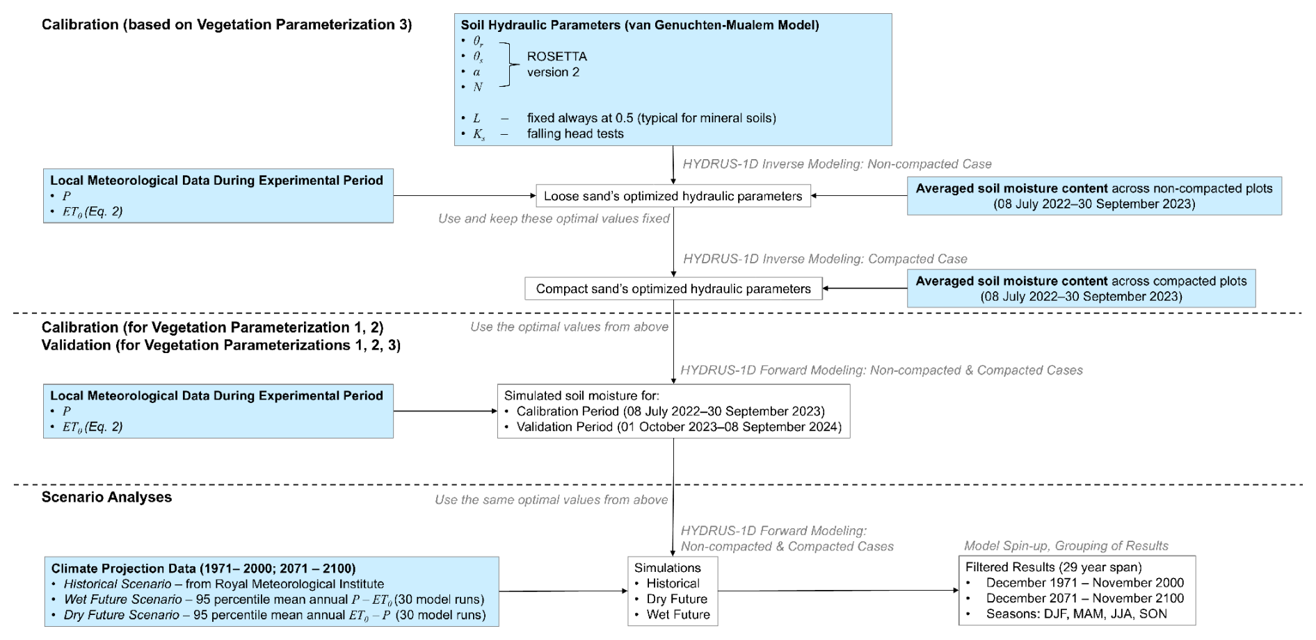
Figure 4 The modeling workflow of this study. Abbreviations: P = precipitation; ET₀ = potential evapotranspiration; DJF = December–January–February; MAM = March–April–May; JJA = June–July–August; SON = September–October–November.

Table 3 Selected wet and dry future scenarios and specifications.

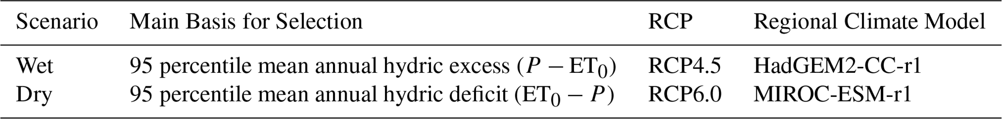
Abbreviations: P = precipitation; ET₀ = Potential Evapotranspiration; RCP = Representative Concentration Pathways.

The future climate projection data are in the form of a 30 run ensemble from regional climate models, used to force the soil water flow models. All these runs, set at the Royal Meteorological Institute at Uccle, Brussels, Belgium (Appendix A – Fig. A2), can be considered representative for inland Flanders (Van Schaeybroeck et al., 2021). They were generated based on the EURO-CORDEX regional climate models under the combined four (RCP 2.6, 4.5, 6.0, 8.5) for the future period 2071–2100. Equal weights were given to these four RCP scenarios. The regional climate model outputs were statistically downscaled via the quantile perturbation method of Willems and Vrac (2011) based on the historical daily meteorological observations in Uccle (1 January 1971 to 31 December 2000).

For the models' spin-up, the results from January–November 1971 were discarded under each run. This is to omit undesired deep percolation recorded a few days after the start of model simulations. The year 1972 was thus defined as the calendar months of December 1971 to November 1972 and so on. Thus, each run spans from the years 1972 to 2000, corresponding to the calendar months of December 1971 to November 2000. With this, equal number of data sets was ensured across seasons in the scenario analyses: 29 data sets each under winter (DJF: December–January–February), spring (MAM: March–April–May), summer (JJA: June–July–August), and autumn (SON: September–October–November). This scheme also applies for the future scenarios.

To represent a wet and a dry future scenario, this study used the 95 percentiles of the mean annual hydric excess (precipitation minus potential evapotranspiration or P − ET₀) and deficit (potential evapotranspiration minus precipitation or ET₀ − P), respectively, from the full ensemble of 30 model runs (Table 3) (Christensen and Christensen, 2003; Van Schaeybroeck et al., 2021). These 95 percentile based scenarios can be interpreted as “high-impact” scenarios, where the future is expected to lie with high likelihood between the current climate and that high-impact scenario.

The whole modeling workflow from setup to scenario analyses is summarized in Fig. 4.

3 Results

3.1 Simulated vs. Observed Soil Moisture Content

Overall, the compacted setup has higher soil moisture than the non-compacted setup, as showed by both observation data and simulations (Fig. 5). At 40 cm depth, these differences are even larger. Moreover, very high soil moisture peaks are more flattened in the compacted setup, reflecting the compacted setup's frequent saturation moments (Fig. 5d). Despite the irrigation at the experiment's beginning, the non-compacted setup was drier than the compact soil. All these reflect the compact layer's role in both experimental plots and simulations.

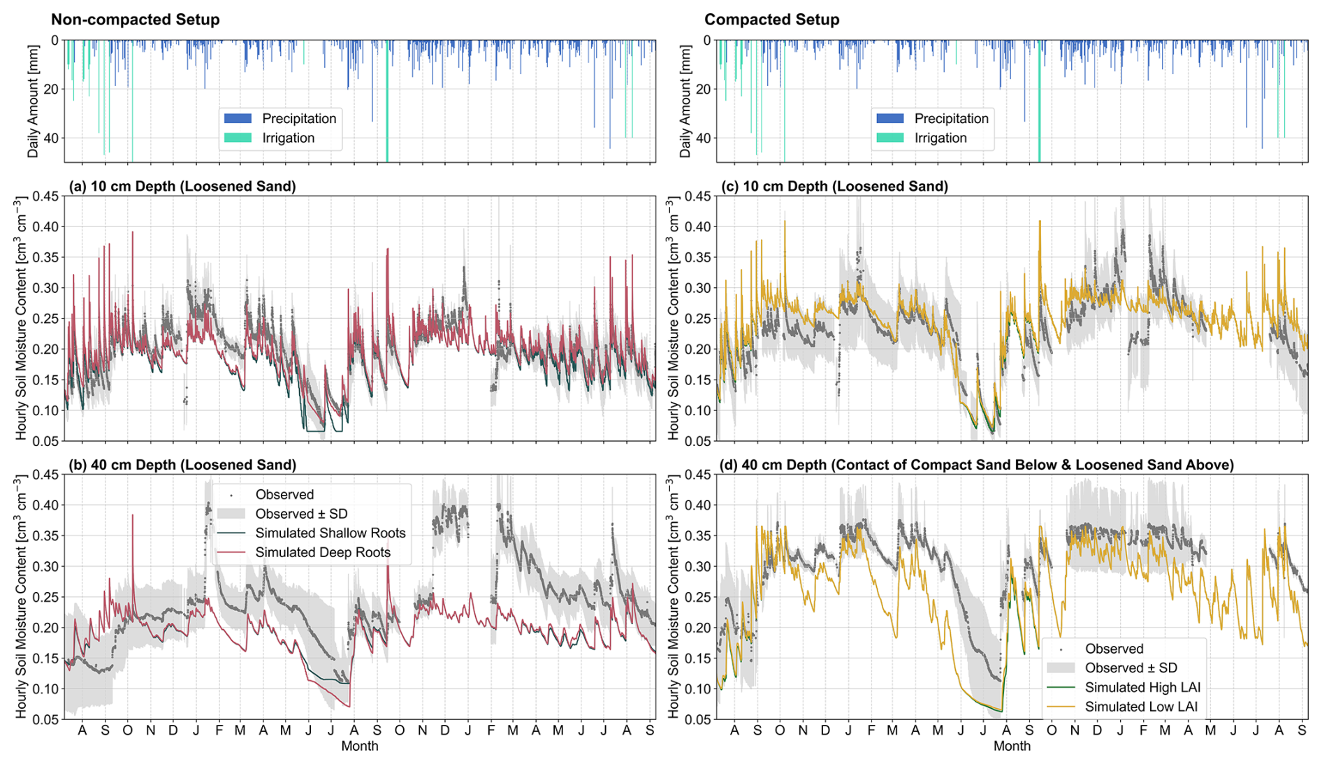
Figure 5 Observed soil moisture content (± standard deviation (SD)) vs. simulated soil moisture content time series at 10 and 40 cm depths under various vegetation parameterizations under calibration (8 July 2022–30 September 2023) and validation periods (1 October 2023–30 September 2024). Performance indicators are listed in Appendix B – Table B5.

At 10 cm depth, the models simulate the soil moisture dynamics well. However, at 40 cm depth, simulations underestimate the soil moisture (Fig. 5b, d). Moreover, the compacted case models simulate a faster decline in moisture content in mid-January 2023 to start of March 2023 (Fig. 5d). This might indicate that the compacted layer's estimated hydraulic conductivity from optimizations is still relatively high. Nearer to the soil surface (Fig. 5a, c), models involving different root depths are closer to observations than the ones with same root depths.

At 10 cm depth (Fig. 5a), the deep rooted non-compacted case model improved the moisture content simulations in mid-May 2023 to mid-July compared to its shallow rooted counterpart. With shallow roots, the model overestimates the root water uptake, leading to its simulations' faster decline than both the observations and deeper root simulations. At 40 cm depth (Fig. 5b), the shallow rooted non-compacted case model underestimated the observed decline in moisture content in June–July 2023. Meanwhile, for the compacted case models (Fig. 5c, d), the differences in LAI yielded very little differences in the simulated moisture contents.

3.2 Scenario Analyses (1972–2000; 2072–2100)

Compared to the historical scenario, the wet scenario depicts slightly higher annual precipitation yet similar annual potential evapotranspiration (Fig. 6a, c). Meanwhile, the dry scenario has a similar annual precipitation yet higher summer potential evapotranspiration. Both future scenarios also show stronger precipitation seasonality (lower in summers and higher in winters) than the historical scenario (Fig. 6b, d).

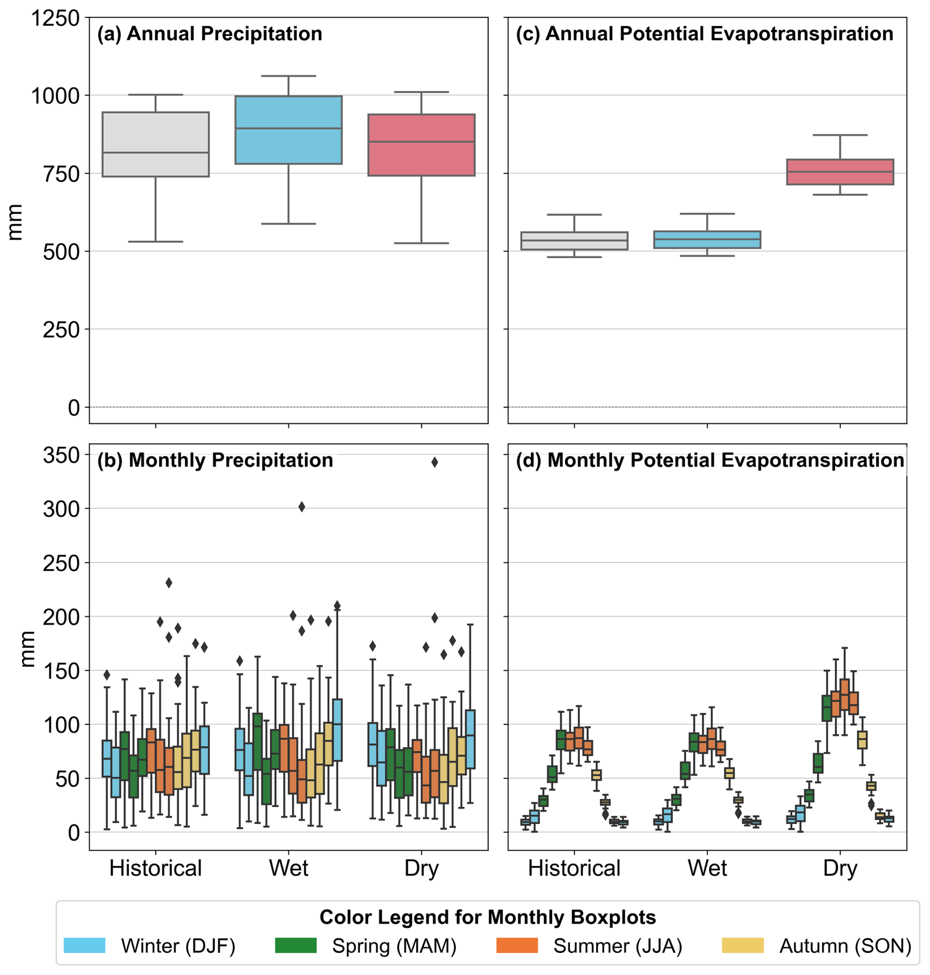
Figure 6 Annual and monthly precipitation and potential evapotranspiration under the historical and wet and dry future scenarios. Boxplots are also colored by seasons. Abbreviations: DJF = December–January–February; MAM = March–April–May; JJA = June–July–August; SON = September–October–November.

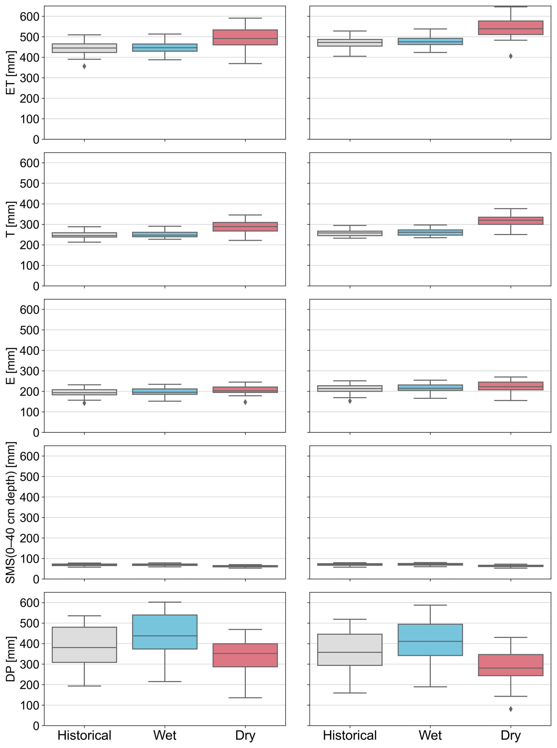
Figure 7 Annual comparison of different hydrometeorological variables for the non-compacted case under historical and wet and dry future scenarios across the three vegetation parameterizations. All the y-axes have the same scale. Abbreviations: ET = actual evapotranspiration, E = actual evaporation, T = actual transpiration, SMS = mean daily soil moisture storage, DP = deep percolation.

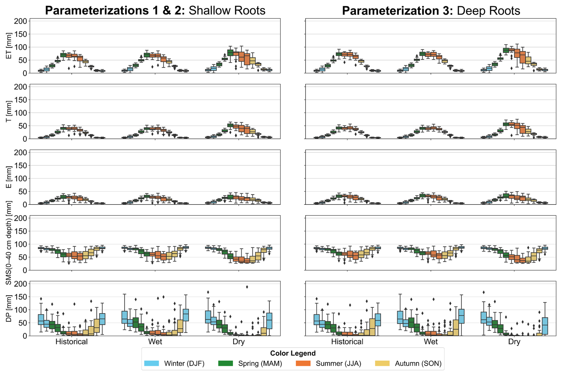
Figure 8 Monthly comparison of different hydrometeorological variables for the non-compacted case under the historical and wet and dry future scenarios. For each scenario under a subplot, 12 boxplots are shown, representing the months of the year from January to December. Sets of boxplots are colored according to their seasons (see legend above). All the y-axes have the same scales. Abbreviations: ET = actual evapotranspiration, E = actual evaporation, T = actual transpiration, SMS = mean daily soil moisture storage, DP = deep percolation, DJF = December–January–February; MAM = March–April–May; JJA = June–July–August; SON = September–October–November.

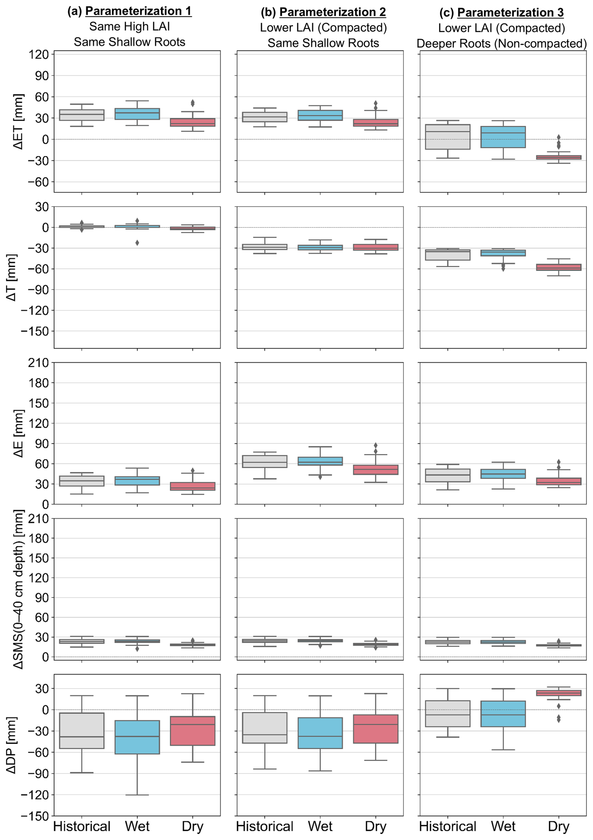
Figure 9 Annual comparison of hydrological variables for the historical and wet and dry future scenarios across vegetation parameterizations (a) 1, (b) 2, and (c) 3. All the y-axes scales are ensured to be consistent. As such, outlier ΔDP values of −196 and −157 were excluded from parameterizations 1 and 2, respectively. Positive values: compacted case > non-compacted case. Negative values: compacted case < non-compacted case. Abbreviations: ET = actual evapotranspiration, E = actual evaporation, T = actual transpiration, SMS = mean daily soil moisture storage, DP = deep percolation. “Δ” signifies subtraction difference between compacted and non-compacted cases' calculated values.

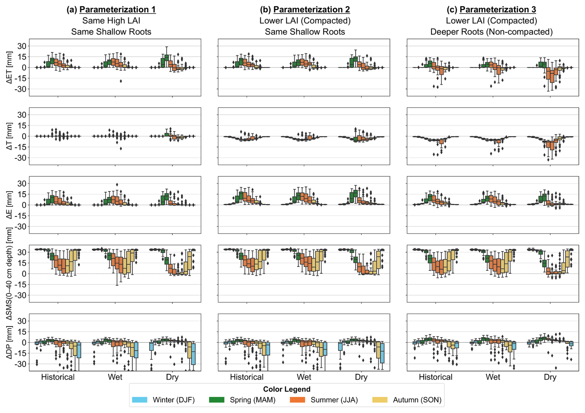
Figure 10 Monthly comparison of hydrological variables for the historical and wet and dry future scenarios across vegetation parameterizations (a) 1, (b) 2, and (c) 3. For each scenario under a subplot, 12 boxplots are shown, representing the calendar months (January–December). Boxplots are also colored by seasons (see legend above). All the y-axes scales are ensured to be consistent. As such, 9 and 6 outlier ΔDP values $<-\mathrm{40}$ were excluded from parameterizations 1 and 2, respectively, belonging to either August, October, or December. Positive values: compacted case > non-compacted case. Negative values: compacted case < non-compacted case. Abbreviations: ET = actual evapotranspiration, E = actual evaporation, T = actual transpiration, SMS = mean daily soil moisture storage, DP = deep percolation. DJF = December–January–February; MAM = March–April–May; JJA = June–July–August; SON = September–October–November. “Δ” signifies differences between calculated values of compacted and non-compacted case.

For the hydrological components (actual evapotranspiration, actual evaporation, actual transpiration, soil moisture storage above the compact layer (i.e., 0–40 cm), deep percolation), the actual fluxes are reported in Figs. 7 and 8. Their results were reported in terms of the annual and monthly differences between the compacted and non-compacted case models in Figs. 9 and 10.

With compaction, water storages in the upper soil profile increase during winter for all vegetation parameterizations and climate scenarios (Fig. 10a, b). However, in the dry climate scenario's summers, both the compacted and non-compacted soils' upper layers dry out to similarly low moisture contents. This is most noticeable for vegetation parameterization 3 with deeper roots and higher LAI in the non-compacted model than in the compacted soil model (Fig. 10c).

For vegetation parameterizations 1 and 2 that assumes same shallow root depths and root density profiles (Fig. 9a, b), actual evapotranspiration and evaporation increase, and deep percolation decreases with compaction. The lower LAI for the compacted case model in parameterization 2 leads to a lower transpiration than the non-compacted case. This is almost fully compensated by higher evaporation in the compacted case model. Thus, vegetation parameterizations 1 and 2 do not exhibit much difference on the simulated impact of compaction on deep percolation.

Under vegetation parameterization 3, the non-compacted case model's deeper rooting leads to more water uptake from the deeper subsoil. This further increases the difference in transpiration between the non-compacted and compacted case models, especially under the dry future scenario (Fig. 9c). This deeper rooting also reduced the uptake from the non-compacted case model's upper depths compared to the shallow rooting from parameterization 2 (Fig. 9b). Thus, more water remained available for evaporation in the non-compacted soil, leading to smaller differences in evaporation losses between the compacted and non-compacted soils (Fig. 9c), than in parameterization 2 (Fig. 9b). Higher transpiration and evaporation from the non-compacted case model also led to its simulated less deep percolation than in parameterization 2. This is shown by parameterization 3's smaller difference in simulated deep percolation between the compacted and non-compacted case models (Fig. 9c). For the historical and wet climate scenarios, more deep percolation is simulated in the non-compacted soil, but the opposite occurs for the dry climate scenario. Thus, whether deep percolation increases or decreases with compaction or after de-compaction depends on how vegetation was parameterized and can be opposite in dry or wet future climate scenarios (Fig. 9c).

In terms of seasonal dynamics, when root depth does not change with compaction (Fig. 10a, b), deep percolation is reduced and delayed for the non-compacted setup after the summer season (especially in November and December). However, if root depth is also adjusted after compaction (Fig. 10c), deep percolation is reduced in the compacted setup in March and April. During this period, the compacted setup has water still draining from the subsoil while root water uptake from deeper layer in the non-compacted setup already starts, reducing deep percolation.

All these key findings of water balance changes due to compaction under various vegetation parameterizations are summarized in Fig. 11.

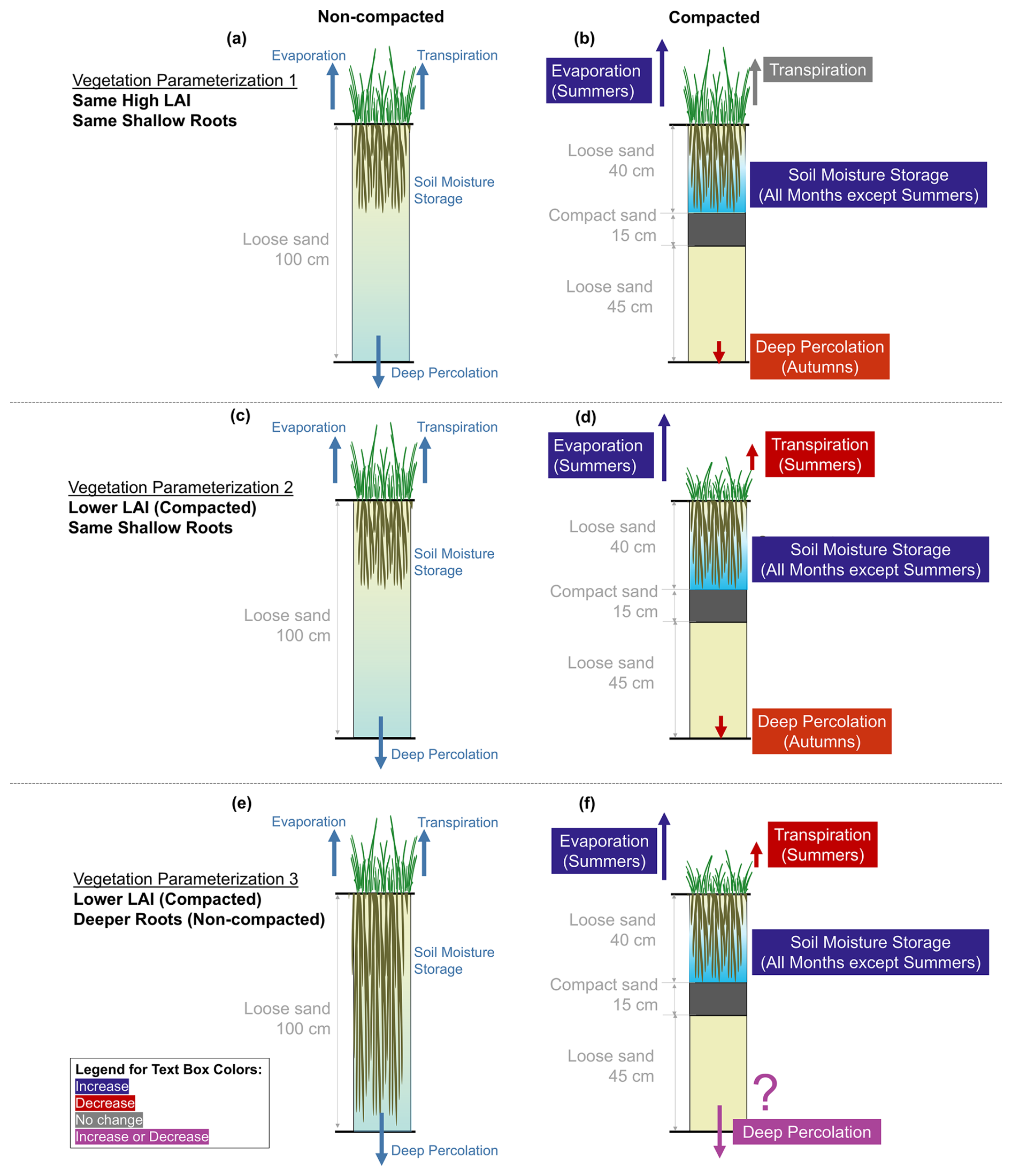
Figure 11 Schematic summary of the impacts of sandy subsoil compaction to the soil hydrology's components under historical and wet scenarios according to the three vegetation parameterizations. The indicated season is when the impact is most significant in a year.

4 Discussion

4.1 Implication on Water Resource Management

Results from the scenario analysis show the effect of both soil compaction and its interaction with the vegetation on the soil water balance (Fig. 11). As per parameterizations 1 and 2 (Figs. 9a, b, 10a, b), a trade-off seemingly exists between soil water retention for vegetation (by leaving the subsoil compacted, based on high soil moisture for the compacted case model) and maximizing groundwater recharge potential (by de-compaction, based on high deep percolation for the non-compacted case model). Considering that compaction reduces vegetation biomass production (i.e., parameterization 2) (Figs. 9b, 10b), de-compaction could promote both groundwater recharge and vegetation productivity. Finally, if the vegetation is allowed to develop a deeper root system in the de-compacted case model (i.e., parameterization 3), de-compaction will not always guarantee higher recharge (Fig. 9c). These abovementioned inferences drawn from these three vegetation parameterizations provide very different and even contrasting overviews of the agricultural water availability's dynamics and sustainability. From these could arise conflicting water resource management strategies tailored to those inferences in this climate change context.

These insights show that while sandy subsoil compaction directly affects both vegetation growth and water balance, the affected vegetation growth also further influences the water balance. Therefore, in hydrological studies involving (de-)compaction, vegetation growth above- and belowground should be dynamically incorporated. With this, field evidence of vegetation growth, root growth and yield, often far lacking in compaction studies, is crucial.

Climate change would likely negatively impact crop production as it could promote more and longer dry (droughts) (Cotrina Cabello et al., 2023; Li et al., 2009; Shanker et al., 2014) and even very wet periods (waterlogging) (Fischer et al., 2023; Tian et al., 2021; Yang et al., 2024). These crop's long-term responses under these contrasting extreme events could also be considered in the hydrological model simulations of future scenarios. This could refine the current understanding of future agricultural water balance even further, including evaporation losses and groundwater recharge.

4.2 Limitations of the Study

Compared to observations at 40 cm depth, the non-compacted case's models severely underestimate the observed soil moisture during wet periods – in two weeks of January 2023 during calibration period (narrow peak) and mid-November to end of December 2023 and mid-February to March 2024 during validation period (wider peak) (Fig. 5b, Appendix A – Fig. A9). The water table could have risen temporarily high enough to saturate these loosened layers at 40 cm depth. The wider soil moisture peak during 2023–2024 is likely due to much higher precipitation (528 mm from 1 October to 31 March) than 2022–2023 (359 mm from 1 October to 31 March) in the site. Unfortunately, the 200 cm deep water table observed from soil profiles during March 2023 and 2024 could have occurred only when the water table had already receded. In flat, low-lying areas, such shallow water table can influence soil hydrological fluxes (Groh et al., 2016) and even vegetation growth (Glanville et al., 2023; Horsnell et al., 2009; Odili et al., 2023; Ridolfi et al., 2006). With this, the feedback loop involving soil compaction, vegetation, and soil water becomes more complex, which, however, is beyond this study's scope.

This study did not also indicate the runoff amounts in the main results. This is because under all scenarios, runoff only occurs for one day just on all compacted case models (i.e., 31 mm on 29 August 1996; 74 and 96 mm in wet and dry August 2096, respectively) whenever an extreme rainfall event occurs under very high antecedent soil moisture conditions. This means that runoff appears to be infrequently simulated, despite reported occurrences of waterlogging in even sandy subsoil compaction (Huang and Hartemink, 2020; Polge De Combret-Champart et al., 2013). This might be due to the difficulty in simulating infiltration-excess runoff as the projected meteorological data have coarse time resolution (i.e., daily), and thus rainfall intensity is not considered (Mertens et al., 2002). This then leads to overestimated infiltration and underestimated runoff in the scenario analyses (Šimůnek and Weihermüller, 2018). Meanwhile, the hourly simulations during the experiments generated runoff for the compacted setups (Appendix B – Table B6), linked to intense irrigation events (40 mm runoff brought by 100 mm irrigation in three hours of 7 October 2022, 27 mm runoff brought by 160 mm irrigation of which 50–60 mm is delivered for six hours every day of 13–15 September 2023; Appendix B – Table B3). Nevertheless, the compaction's role on runoff generation is still clear as only the compacted case models generated runoff in both the experiments and scenario analyses.

5 Conclusion

To assess both compaction's hydrological impact and de-compaction's effectiveness to promote infiltration and groundwater recharge, soil water flow modeling has long been performed to quantify its impacts on soil water balance. Here, for sandy subsoils, this study showed that interpretations and insight from these model simulations can drastically change with the level of understanding on the vegetation's role in the study site.

By assuming same root depths and LAI, compaction promotes more soil storage and thus more evaporable water while reducing and delaying deep percolation. Lower LAIs for the compacted setups further lead to higher evaporation yet lower transpiration than the compacted case with unadjusted LAIs. Finally, if root depths increased also for non-compacted setups, evaporation still increased for the compacted case while transpiration decreased. However, deep percolation can increase or decrease with compaction depending on the year (Fig. 11). Thus, having different results across various vegetation parameterizations highlights the need for more accurate parameterization of vegetation's growth to achieve more robust and confident conclusions. In other words, to properly assess sandy subsoil (de-)compaction's hydrological impacts, the vegetation's role must be clearly understood.

Appendix A: Additional Figures

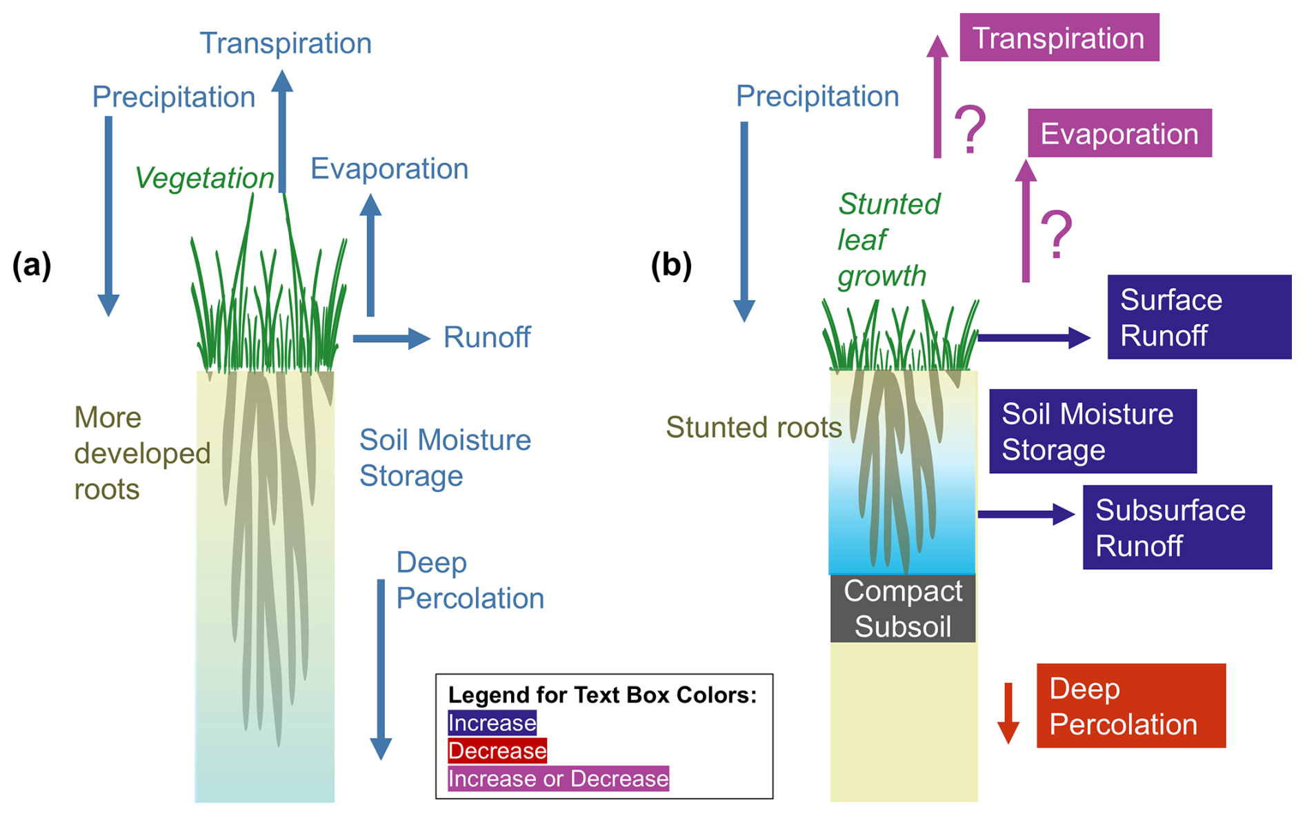
Figure A1 Summary of compaction's previously known impacts on soil water hydrology, comparing (a) non-compacted case and (b) compacted case with compact subsoil.

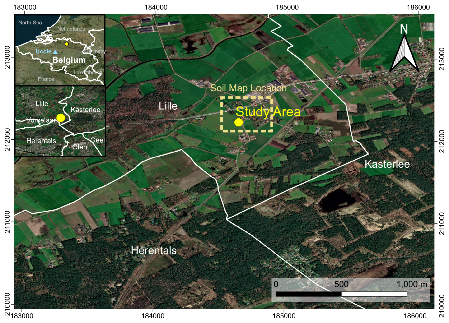
Figure A2 Location map showing the study area, the location region of soil map (Appendix A – Fig. A4), and nearby countries (top inset) and municipality (bottom inset). Coordinate system: EPSG 31370 – BD72/Belgian Lambert 72. Basemap: Bing Virtual Earth (© Microsoft, 2012).

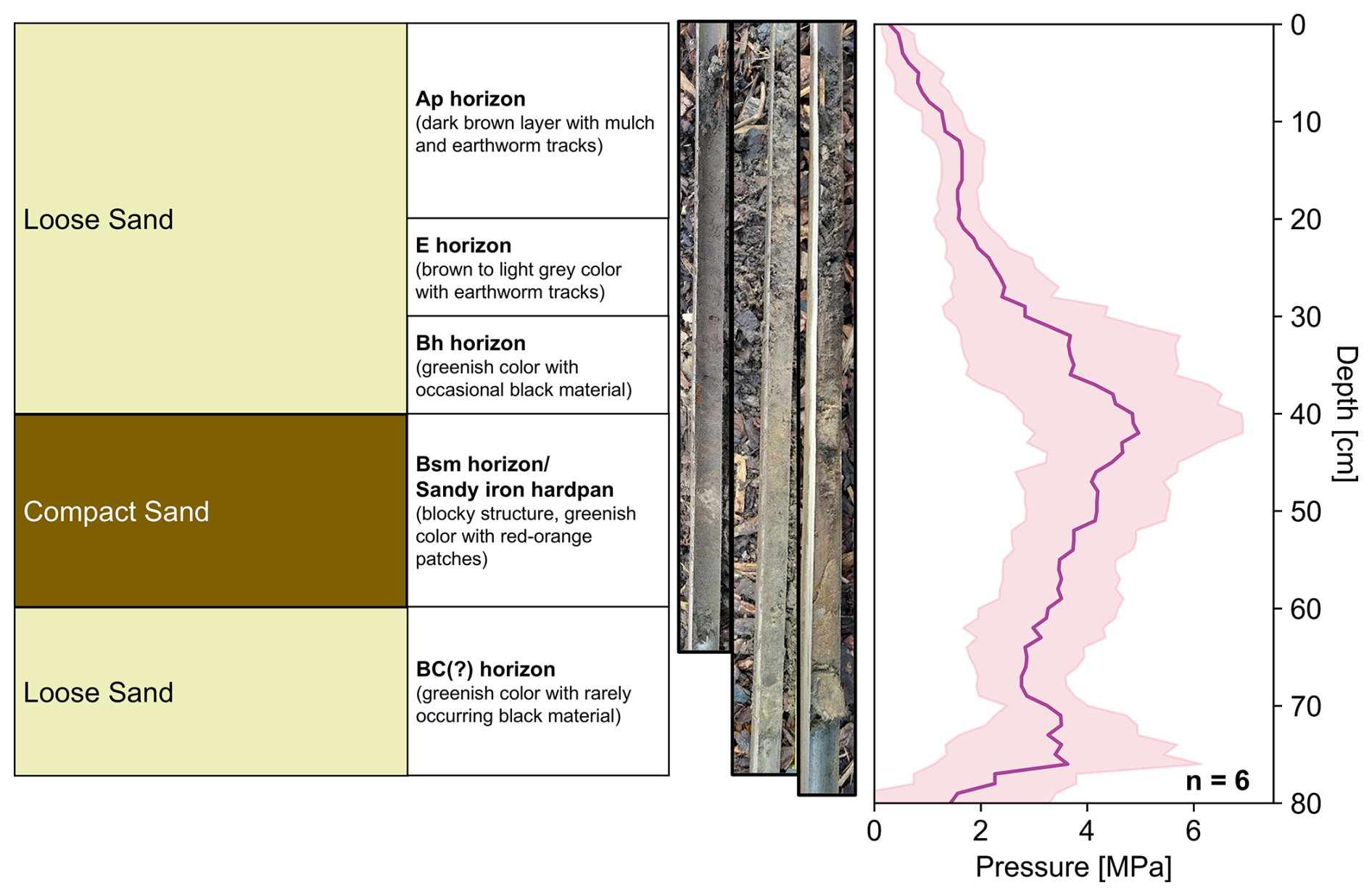
Figure A3 Characterized soil profiles taken outside the plots and the corresponding penetrologger profile.

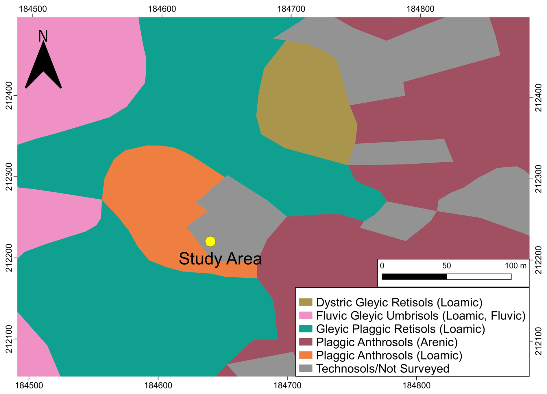
Figure A4 Soil types present in the vicinity (based on the boxed region in Appendix A – Fig. A2). The soil map data are based on Dondeyne et al. (2015). Coordinate system: EPSG 31370 – BD72/Belgian Lambert 72.

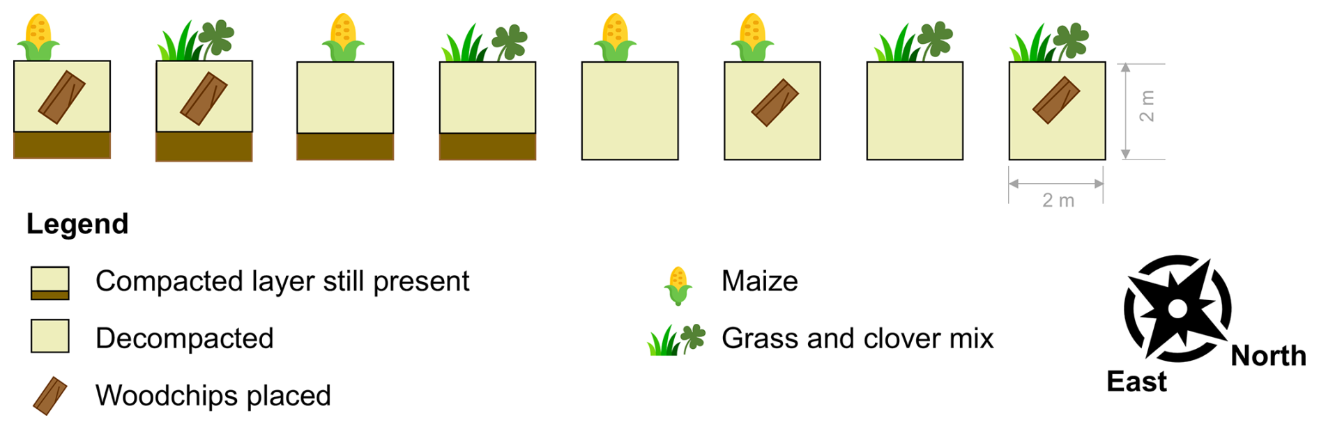
Figure A5 Experimental Plots in the Site, showing various treatments such as presence and absence of the compact layer, vegetation type (maize, grass-clover mixture), and application of woodchips for certain plots.

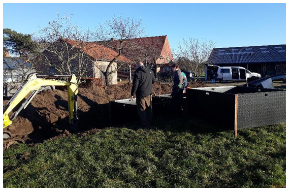
Figure A6 Excavation works during set up of experimental site, showing the black impermeable plastic boxes and the crane used for de-compaction.

Figure A7 General Timeline of the Experimental Activities.

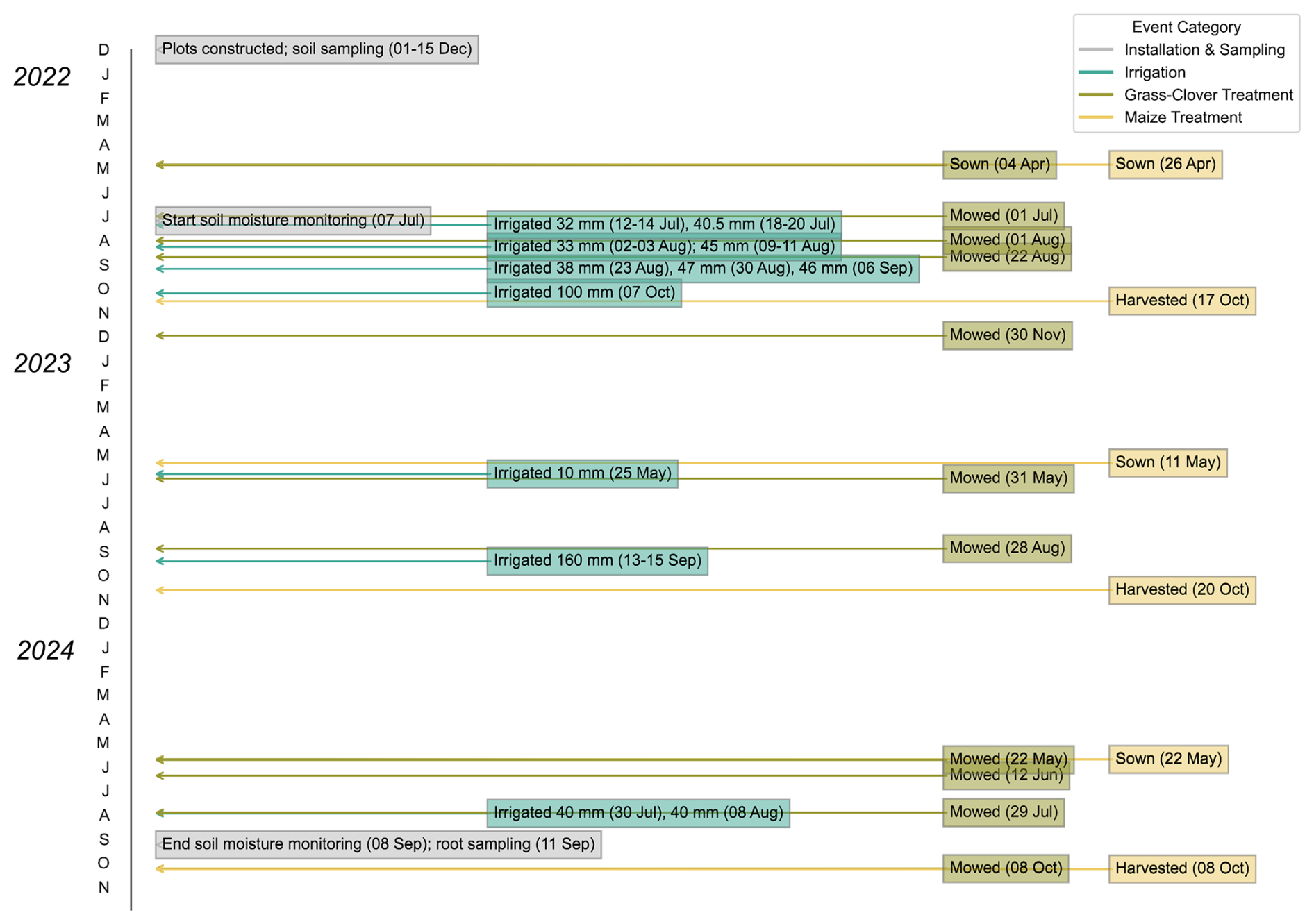
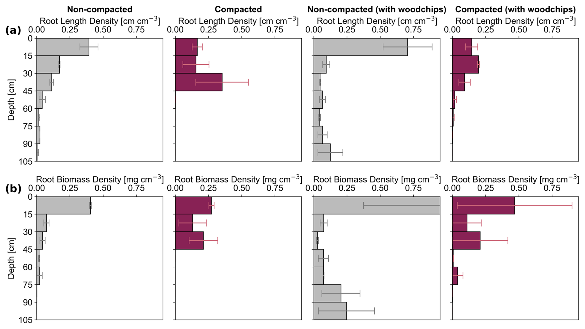
Figure A8 (a) Mean root length and (b) biomass densities (± standard deviation) across individual plots of grass-clover mixtures (n=2). Note that the non-compacted plot with woodchips' 0–15 cm depth has a mean root biomass density exceeding 1.00 (i.e., 2.83 ± 2.46).

Figure A9 Soil moisture content measurements for each plot and averages across them.

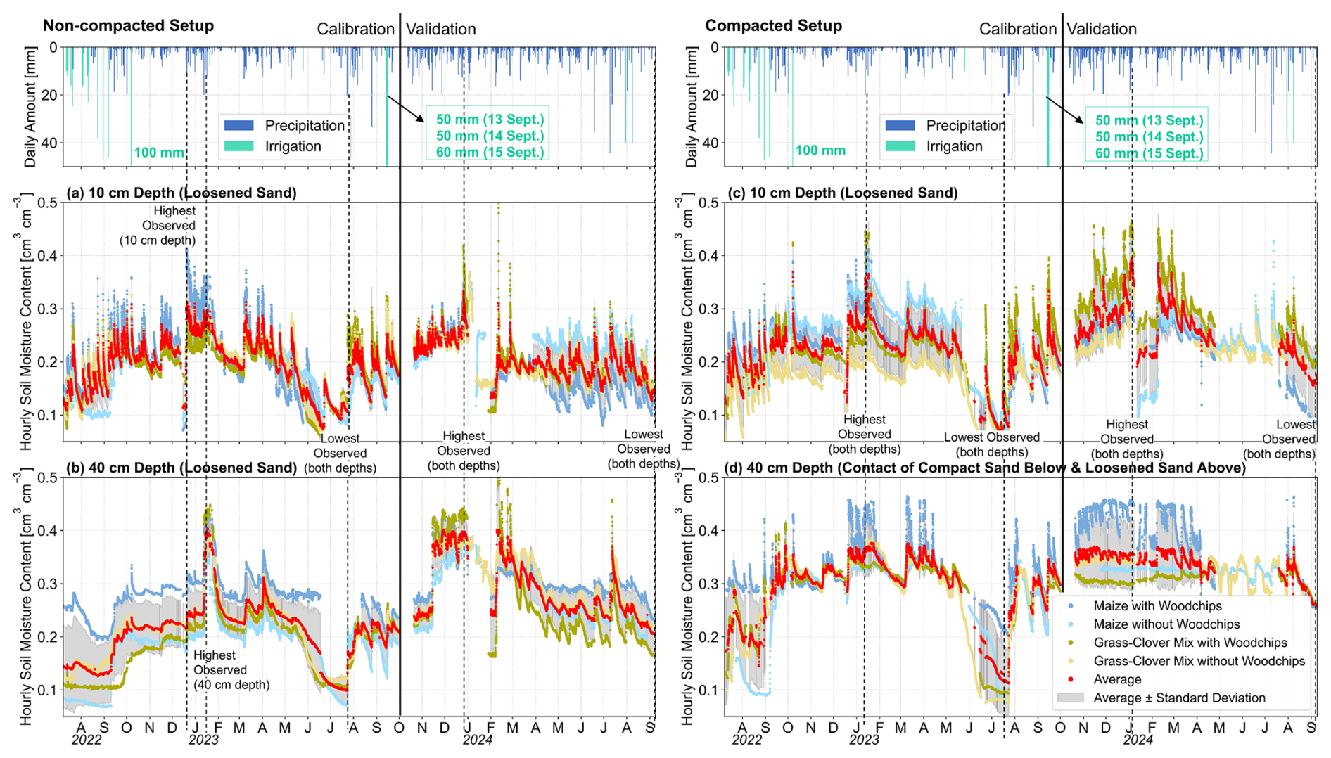
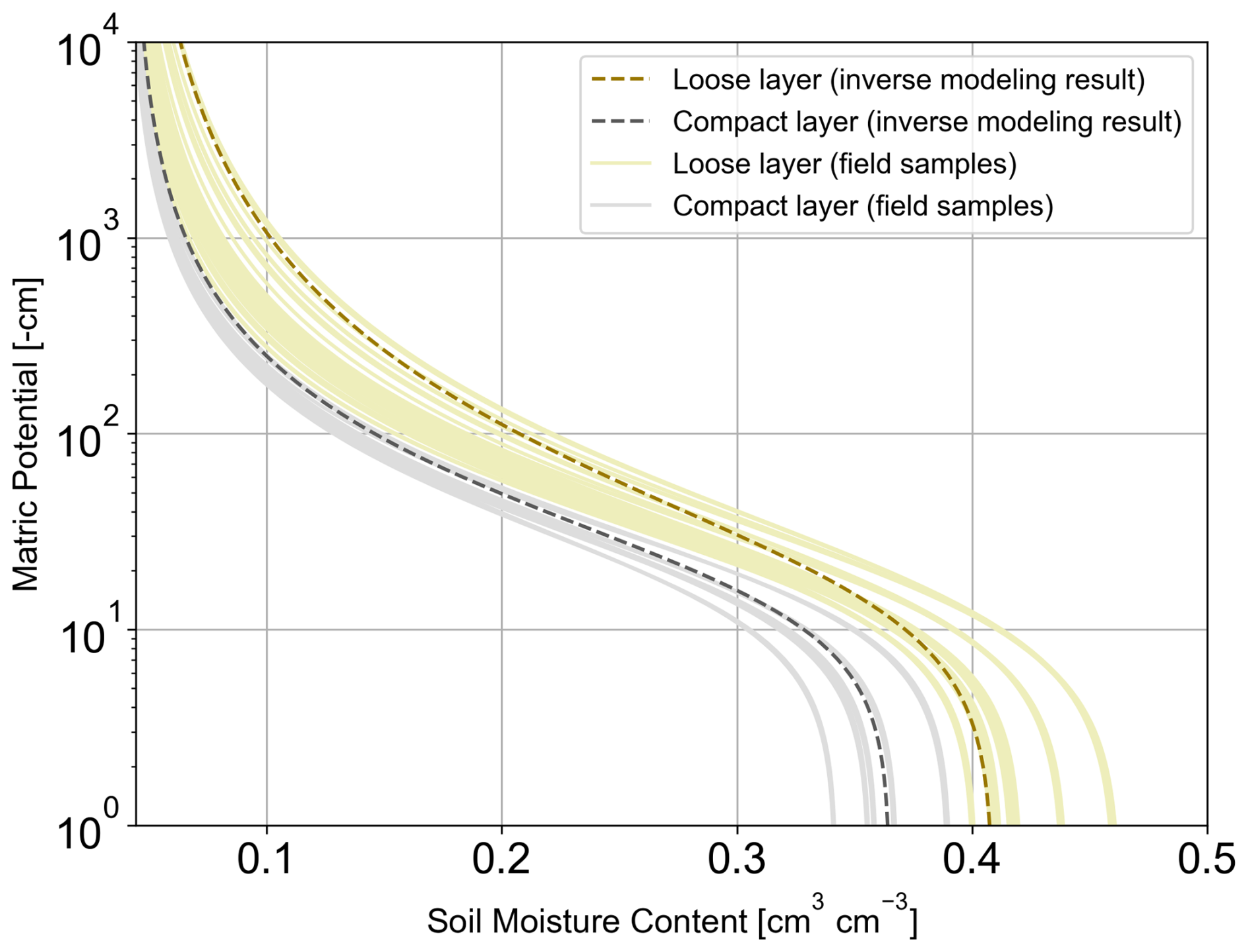
Figure A10 Water retention curves for loosened and compact sand layers based on optimization from inverse modeling and on field samples whose properties were inferred from ROSETTA.

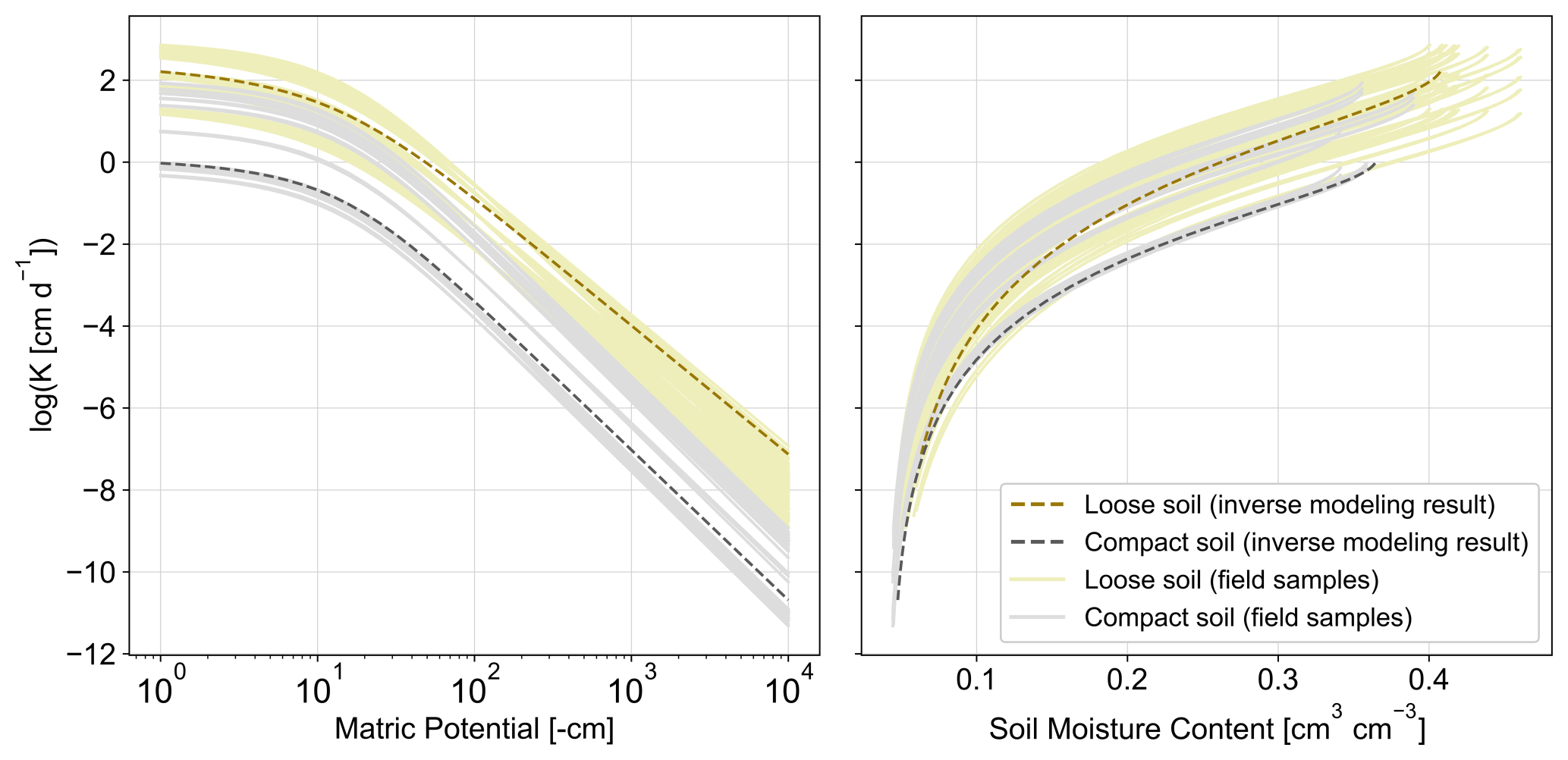
Figure A11 Conductivity curves (log K vs. pF (left), log K vs. θ (right)) for both loosened and compact sand layer based on optimization from inverse modeling and on field samples whose properties were inferred from ROSETTA and K_s measurements (falling head method).

Appendix B: Additional Tables

Table B1 Numerical hydrological modeling studies on soil (de-)compaction's hydrological impacts in small-scale sites.

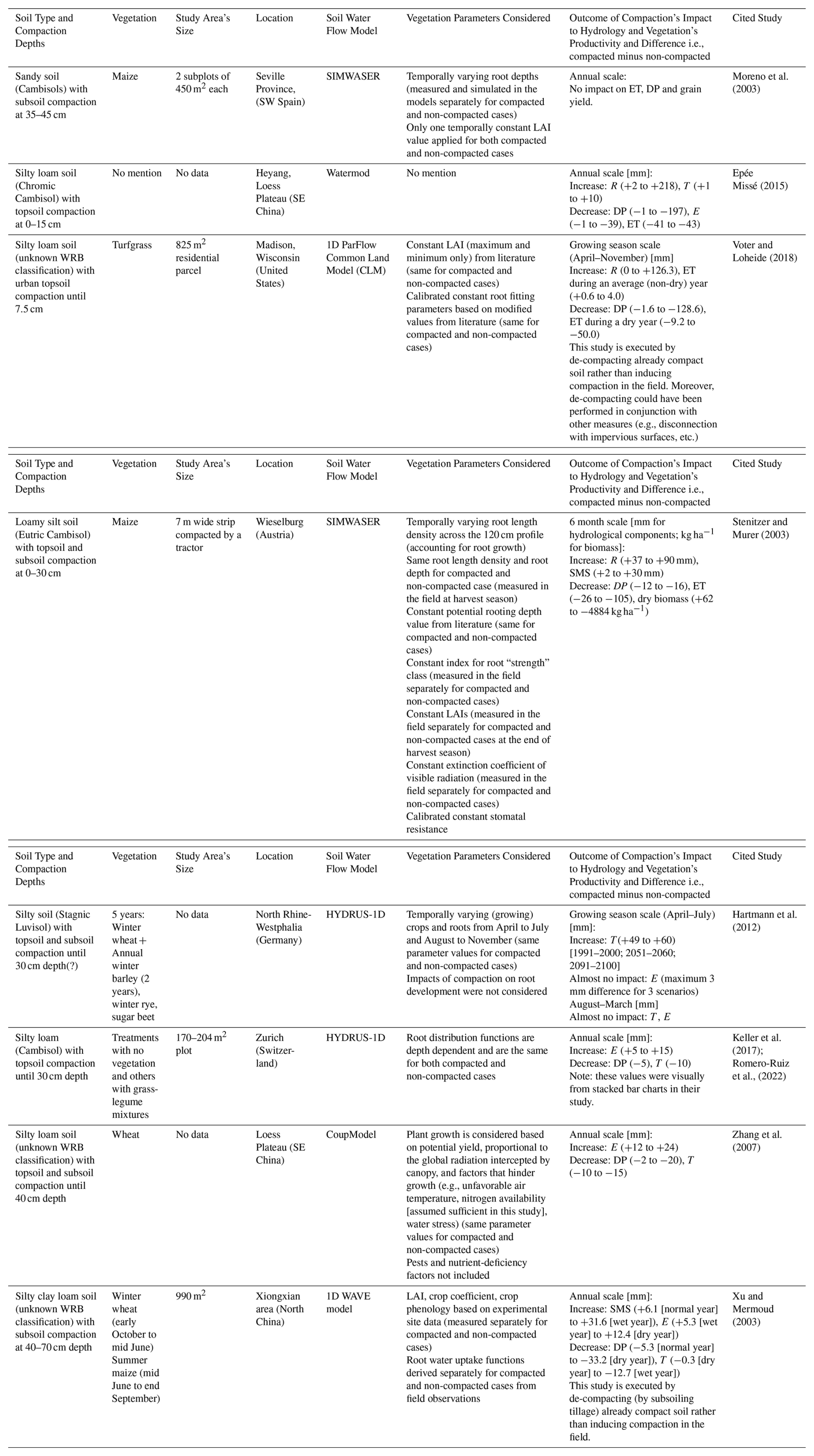
Table B2 Irrigation amounts applied during the study period (July 2022–September 2024) and based historical events in Herentals (closest active meteorological station from the study site) (Flemish Environment Agency, 2021).

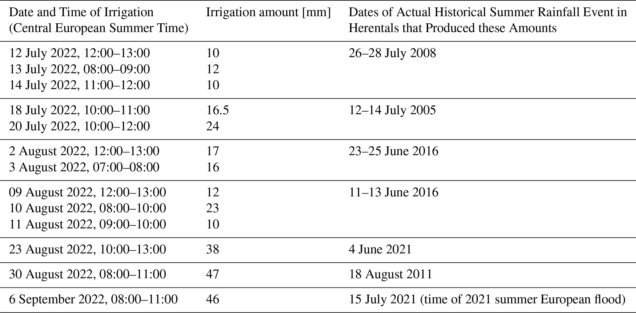
Table B3 Other applied irrigation amounts applied (not based on historical events).

Table B4 Constraints used for inverse modeling.

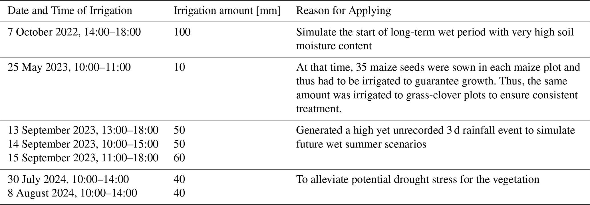
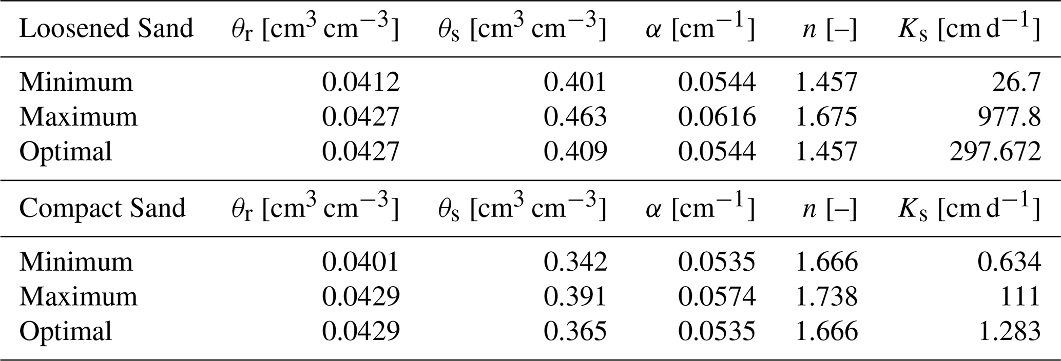
Table B5 Performance indicators of the models based on the presence of compaction, observation point depths, and model parameterizations.

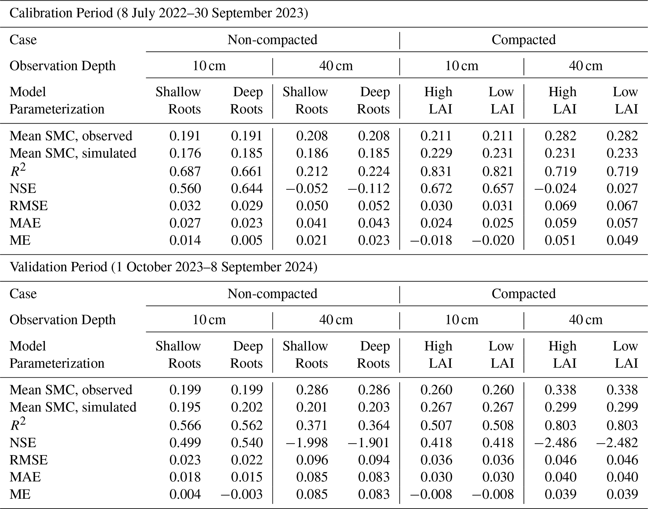
Abbreviations: SMC = Soil Moisture Content [cm³ cm⁻³]; R² = Coefficient of Determination; NSE = Nash-Sutcliffe Efficiency; RMSE = Root Mean Squared Error [cm³ cm⁻³]; MAE = Mean Absolute Error [cm³ cm⁻³]; ME = Mean Error [cm³ cm⁻³].

Table B6 Water budget results for the three vegetation parameterizations during the experimental period. All units are in mm.

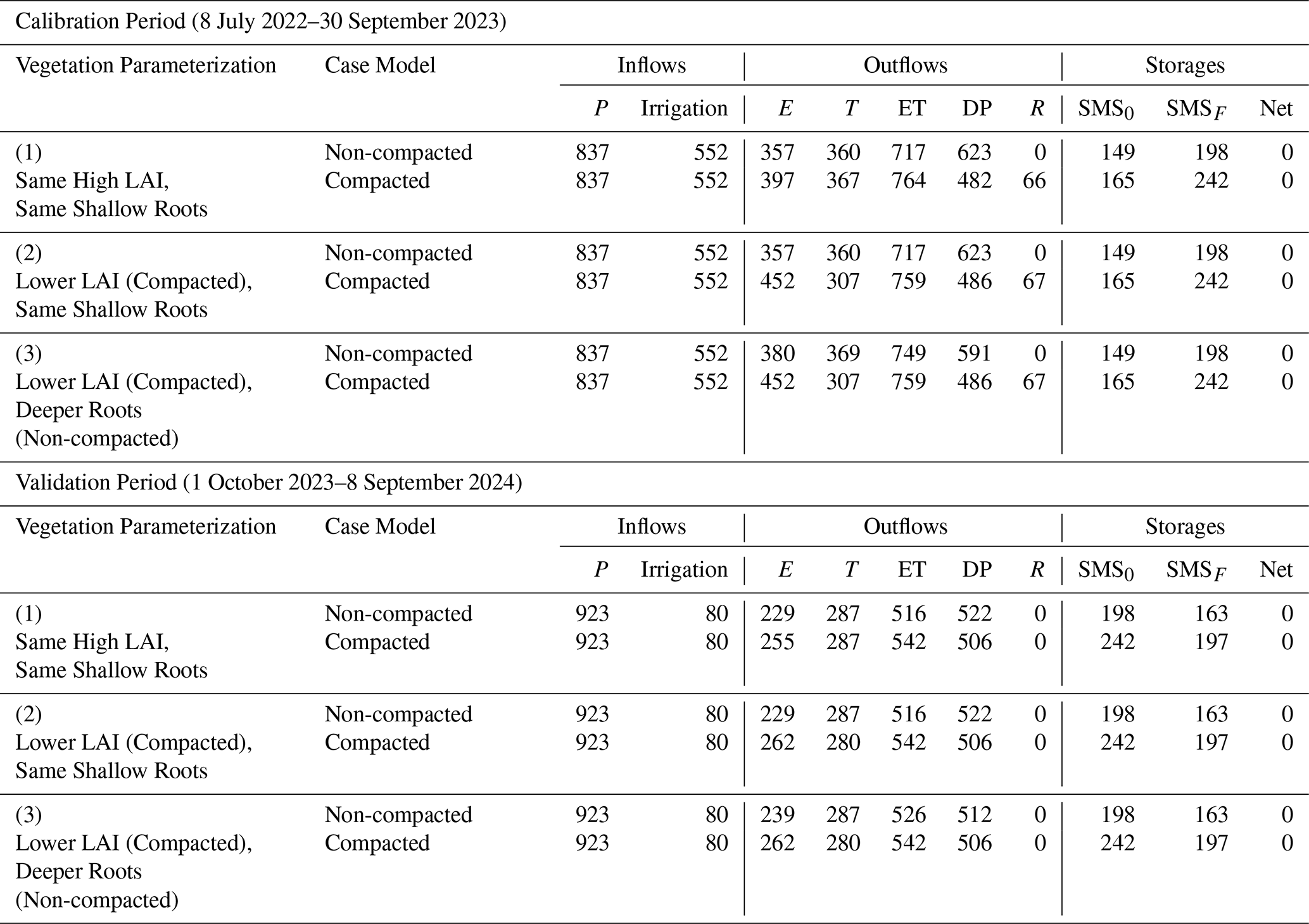
Abbreviations: P = precipitation, E = actual evaporation, T = actual transpiration, ET = actual evapotranspiration, DP = deep percolation, R = runoff, SMS₀ = initial soil moisture storage, SMS₀ = initial soil moisture storage = final soil moisture storage, $\mathrm{Net}=(P+\mathrm{Irrigation})-(\mathrm{ET}+\mathrm{DP}+R)-({\mathrm{SMS}}_F-{\mathrm{SMS}}_{\mathrm{0}}$).