Assessing soil fertilization effects using time-lapse electromagnetic induction

Adding mineral fertilizers and nutrients is a common practice in conventional farming and is fundamental to maintain optimal yield and crop quality; nitrogen is the most applied fertilizer and is often used excessively, leading to adverse environmental impacts. To assist farmers in optimal fertilization and crop management, non-invasive geophysical methods can provide knowledge about the spatial and temporal distribution of nutrients in the soil. In recent years, electromagnetic induction (EMI) has been widely used for field characterization, to delineate soil units and management zones, or to estimate soil properties and states. Additionally, ground-penetrating radar (GPR) and electrical resistivity tomography (ERT) have been used in local studies to measure changes in soil properties. Unfortunately, the measured geophysical signals are confounded by horizontal and vertical changes in soil conditions and parameters, and the individual contributions of these conditions and parameters are not easy to disentangle. Within fields, and also between fields, fertilization management might vary in space and time, and, therefore, the differences in pore fluid conductivity caused directly by fertilization or indirectly by different crop performance make the interpretation of large-scale geophysical surveys over field borders complicated. To study the direct effect of mineral fertilization on the soil electrical conductivity, a field experiment was performed on 21 bare-soil plots with seven different fertilization treatments. As fertilizers, calcium ammonium nitrate (CAN) and potassium chloride (KCl) were chosen and applied in three dosages. Soil water content, soil temperature, and bulk electrical conductivity were recorded continuously over 450 d. Additionally, 20 EMI, 7 GPR, and 9 ERT surveys were performed, and on days of ERT measurements, soil samples for nitrate and reference soil electrical conductivity measurements were taken. The results showed that (1) the commonly used CAN application dosage did not impact the geophysical signals significantly. (2) EMI and ERT were able to trace back the temporal changes in nitrate concentrations in the soil profile over more than 1 year. (3) Both techniques were not able to trace the nitrate concentrations in the very shallow soil layer of 0–10 cm, irrespective of the low impact of fertilization on the geophysical signal. (4) The results indicated that past fertilization practices cannot be neglected in EMI studies, especially if surveys are performed over large areas with different fertilization practices or on crops grown with different fertilizer demands or uptakes.

1 Introduction

To meet the challenges of a growing world population and to cope with the negative impacts of climate change, it is important to develop innovative and sustainable agricultural management strategies that increase crop yields while maintaining healthy soils (Shah and Wu, 2019). Mineral nitrogen (N) or potassium fertilization is thereby essential in conventional farming to ensure high yields and optimal crop quality. Additionally, care must be taken to maintain optimal timing and the right amounts of fertilizers to avoid pollution of groundwater and surface water (Galloway et al., 2004; Bouwman et al., 2005; Olatuyi et al., 2012) and to reduce emissions to the atmosphere, which could negatively affect the climate (Butterbach-Bahl et al., 2013). The plant-specific nitrogen demand depends on the crop, while the required fertilization amounts also depend on the nitrogen replenishment from the soil (Drücker, 2016). Therefore, for sustainable agriculture with improved plant performance, it is highly important to develop tools for soil nitrogen mapping and monitoring in which measurements are not restricted to the soil surface but rather provide information on local heterogeneities within the root zone and estimate the available fertilizer present in the soil profile. As stated by Kuang et al. (2012), precision agriculture explicitly considers field heterogeneities of soil properties and crop status by dividing the field into small-scale areas with the same properties and/or crop development. This allows specific management of these sub-areas depending on their needs in terms of soil management (e.g., tillage or plant to be grown), fertilization, pest control, and irrigation (Hinck et al., 2016; Koch et al., 2023).

Among the agrogeophysical methods, electromagnetic induction (EMI) has been proven to be an excellent method to delineate crop management zones. For example, Hedley et al. (2004) performed EMI surveys of a pastoral–cropping farming system over a year and used these data to delineate zones of different apparent soil electrical conductivity (ECa). Further, the authors compared those zones with soil units of a conventional soil map, and the results indicated that the ECa map related well to soil textural classes, allowing accurate grouping of different soil types. King et al. (2005) focused their study on the evaluation of yield maps and EMI data to determine management zones within fields. The results showed that the management zones identified by both methods provided useful information for the provisional delineation of soil type boundaries and crop management zones. A comparable study was performed by Serrano et al. (2022), who used EMI data and altimetry surveys in six experimental pasture fields to establish maps with three homogeneous management zones (HMZs) (low, intermediate, and high potential). The normalized difference vegetation index (NDVI) obtained from a proximal optical sensor and soil and biomass sampling were used to validate these HMZs. A further advancement was proposed by Brogi et al. (2019), who used EMI data and a supervised classification scheme to establish, together with soil profile information and soil textural data, a high-resolution soil map of a small agricultural area in Germany. In a follow-up paper, Brogi et al. (2021) used this map to simulate crop growth in the area and compared the simulation results with simulations based on available soil maps. For the validation of the simulation results, leaf area index (LAI) data from remote sensing were used. The findings indicated that the EMI-based soil map demonstrated superior performance compared to the conventional soil maps utilized in the study area. Recently, new avenues have been opened with regard to the use of EMI, where either new interpretation approaches have been employed or EMI data have been combined with other non-invasive sensor data. For example, in a study by O'Leary et al. (2024), EMI data gathered were clustered with a neural network to demonstrate the correlation between soil electrical conductivity with soil texture. The results showed that the clustering outperformed the classical simple correlations between measured EMI and soil texture. As an example for sensor combination, van Hebel et al. (2021) combined ground-based EMI and aerial crop data (NDVI) from drones to delineate field-specific management zones, which they interpreted with soil attribute measurements of soil texture, bulk density, and soil water content. Finally, they compared those zones with different yield and nitrate concentrations in the soil after potato (Solanum tuberosum L.) cultivation.

Although all these studies successfully demonstrated the potential to derive soil properties or to delineate soil or crop management zones by means of geophysical methods such as EMI, EMI measurements also have limitations as the measurement of the apparent electrical conductivity (ECa) is impacted by soil temperature (e.g., Corwin and Lesch, 2005), soil mineral surface polarization (chargeability) (Saey et al., 2013), profile soil water content (e.g., Huang et al., 2016), and pore water salinity (Triantafilis et al., 2003). Soil temperature effects on the EMI signal have been widely studied, and correction formulas have been proposed by, e.g., Corwin and Lesch (2003) for EMI data measured at different times and with variable temperatures. Additionally, differences in soil particle properties (e.g., clay content) and/or soil water content (SWC) are often the targets under investigation in EMI surveys in non-saline soils (Kachanoski et al., 1988; Triantafilis and Lesch, 2005; Saey et al., 2009; Robinson et al., 2012; Rudolph et al., 2016). However, confounding factors such as the impact of changes in pore water conductivity resulting from differences in fertilization or fertilizer uptake on different crop performances have mostly been neglected.

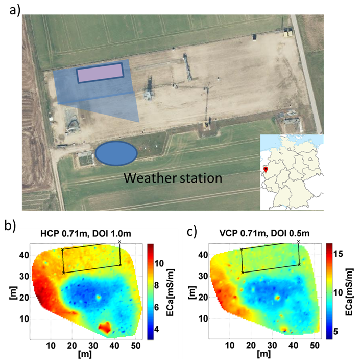
Figure 1 (a) Overview of the Selhausen test site (map adapted from ©Google Earth, 2017). The location of the weather station is marked with a blue circle, while the pre-experimental EMI survey area is shown by the violet plane. In the lower right of panel (a) is the location of the test site in Germany, marked with a red dot. EMI-measured ECa maps [mS m⁻¹] for (b) horizontal-loop HCP, 0.71 m mode, and (c) vertical-loop VCP, 0.71 m mode. The pink box in panel (a) and the black rectangles in panels (b) and (c) indicate the domain in which the field trial covering the 21 plots is set up.

Commonly used organic or inorganic fertilizer releases charged molecules or ions (e.g., ${\mathrm{NH}}_{\mathrm{4}}^{+}$, ${\mathrm{NO}}_{\mathrm{3}}^{-}$, ${\mathrm{Ca}}_{\mathrm{2}}^{+}$, or dissolved organic carbon (DOC)) into the soil, affecting the soil electrical conductivity and, therefore, also the EMI signal. For example, Eigenberg et al. (2002) observed that applied compost, manure, and mineral N fertilizer resulted in consistently higher electrical conductivities in arable fields and indicated the potential of EMI methods to provide reliable indicators of soluble-N gains and losses. Eigenberg and Nienaber (2003) performed EMI measurements to identify areas of nutrient buildup beneath an abandoned compost site, and the resulting ECa maps – or, to be precise, the structures with high ECa – were in good agreement with the former row locations of the compost. Hereby, the identified historical compost rows showed significantly increased soluble salts (1.6 times greater), ${\mathrm{NO}}_{\mathrm{3}}^{-}$ (6.0 times greater), and Cl⁻ (2.0 times greater) compared with the area between the rows. Additionally, the authors also used yearly repeated EMI measurements to display annual changes associated with nutrient movement and transformations. In conclusion, Eigenberg and Nienaber (2003) stated that the correlation between EMI measurements and soil core analyses for ${\mathrm{NO}}_{\mathrm{3}}^{-}$, N, Cl⁻, and EC provided ancillary support for the EMI methods. Kaufmann et al. (2019) showed, based on EMI measurements in long-term field experimental sites with different fertilization and irrigation, the legacy effect on EMI data, offering new potential in detecting and understanding the effects of agricultural management. Recently, Blanchy et al. (2020) used time-lapse EMI and electrical resistivity tomography (ERT) measurements to demonstrate their applicability to studying water content changes induced by different commonly applied agricultural practices, such as the introduction of cover crops, compaction, irrigation, tillage, and N fertilization. The results showed that different N application rates had a significant effect on the yield and leaf area index but only ephemeral effects on the dynamics of electrical conductivity, mainly after the first fertilizer application. As the EMI signal was mainly impacted directly after N fertilization, one can suggest the hypothesis that even common fertilization rates directly impact the measured ECa signal substantially.

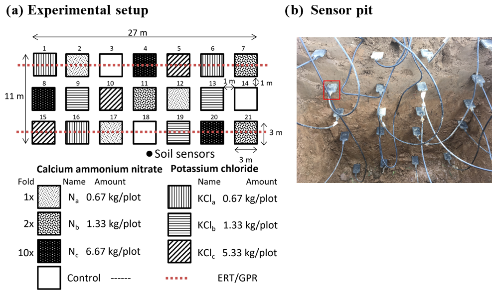
Figure 2 (a) Sketch of the experimental setup with control treatment (and the different dosages of calcium ammonium nitrate (N) and potassium chloride (KCl)). Small letters  – a, b, and c – indicate dosages. ERT and GPR lines are indicated with the dashed red lines, and the location of the in situ soil sensors is indicated with a black dot. The upper transect is transect 1, and the lower transect is transect 2. (b) An image from the installation setup of the soil sensor data measuring soil water content, soil electrical conductivity, and soil temperature measurements (red square marks a defect sensor).

Even if there are indications that commonly used fertilization rates impact EMI ECa measurements to an extent that is not negligible in the interpretation, comprehensive studies of the impact of varying fertilizer applications on EMI are currently lacking. Therefore, we intend, in this study, to close this gap by analyzing the effect of different N and potassium fertilization rates on the measured EMI signal using time-lapse data measured over differently fertilized bare-soil plots. For a better interpretation, the EMI measurements were accompanied by ERT and ground-penetrating radar (GPR) measurements as those systems can provide additional information on water content (GPR) or highly resolved vertical EC information (ERT). For ground-truthing, soil samples were taken, and the nitrate content and soil bulk electrical conductivity (${\mathrm{EC}}_{\mathrm{e}}^{\mathrm{soil}}$) were measured at the times of the geophysical surveys. Finally, sensors automatically recorded the bulk soil EC, soil water content, and soil temperature at different depths to help in interpreting the measured geophysical data.

2 Materials and methods

2.1 Selhausen test site

The experiment was conducted at the test site Selhausen, Germany (Fig. 1), which is part of the TERENO (TERrestrial ENvironmental Observatories) Eifel–Lower Rhine observatory in North Rhine-Westphalia, Germany (Pütz et al., 2016; Bogena et al., 2018). The site consists of Quaternary sediments covered by loess and is located at a transition zone between the upper and lower terraces of the Rhine–Meuse river system. The main textural fraction, accounting for 55 %–67 % across all horizons, is silt (Weihermüller et al., 2007). Annual precipitation is 715 mm, and mean annual temperature is 10.2 °C (Rudolph et al., 2015). The groundwater depth shows seasonal fluctuation, but no groundwater was detected in the first 3 m of the subsurface. In the last years, several geophysical studies have been performed at this test site (e.g., Jonard et al., 2011; Busch et al., 2014; von Hebel et al., 2014; Kaufmann et al., 2020), and, based on these previous geophysical studies, a location at the lower terrace was chosen to be best suited for the experiment as low natural soil heterogeneity was expected there (blue box in Fig. 1a). In order to prove low soil heterogeneity and uniformity in soil ECa, an EMI survey was performed on 2 March 2017 (results shown in Fig. 1b and c). Based on those maps, the experimental plots were established in the southern end of the field site, characterized by low variability in soil ECa (black box in Fig. 1b and c).

Table 1 Overview of all measured parameters and methods.

2.2 Field experiment

To measure the effect of different fertilizers and dosages over time on the EMI-measured ECa data, a field experiment with seven different treatments was established. The treatments consisted of a control (no fertilizer applied), two different commercial fertilizers, calcium ammonium nitrate (CAN) with 26 % N content, and potassium chloride (KCl) with 40 % K. For the CAN and KCl treatments, three different dosages (normal (a), double (b), and 10-fold (c)) were selected. A normal N fertilization level was defined as 190 kg N ha⁻¹, resulting in application dosages of 0.67, 1.33, and 6.67 kg per plot for (a), (b), and (c), respectively. KCl had equal dosages for (a) and (b), but for treatment (c), the amount had to be reduced to 5.33 kg per plot as this was the maximum amount to be diluted in the water used for irrigation. Each of the seven treatments was triplicated and randomly assigned to the 21 plots of 9 m² (3 m × 3 m) in size. Plots were separated by 1 m from each other (see Fig. 2a). The fertilizers were dissolved in water (10 to 30 L depending on fertilizer dosage) and homogeneously applied with commercial watering cans on 3 April 2017. This date is later used as reference day 0, and all following days are denoted in days after fertilization (DAF). To monitor the effect of fertilization over time, 20 EMI measurements were conducted over a period of 485 d (DAF 485) (see Table 1). As mentioned, GPR and ERT measurements were also performed to support the interpretation of the fertilizer effects on the EMI-measured ECa.

For a permanent record of SWC [m³ m⁻³], soil temperature [°C]  and bulk electrical conductivity [mS m⁻¹], 20 sensors (5TE, 5TM, and ECH2O-TE) from Decagon Devices Inc. (Pullman, WA, USA) were installed (Fig. 2b). The installation depths of the sensors were 10, 20, 30, 40, and 60 cm, whereby four sensors were always installed at each depth, with a separation of 10 cm. As not all sensors measure ${\mathrm{EC}}_{\mathrm{e}}^{\mathrm{soil}}$, care was taken to install at least two sensors capable of measuring EC at each depth. The sensor data were logged hourly and daily averaged afterwards. To avoid any N losses by plant uptake, the plots had to be cleared of vegetation. Therefore, the area was treated three times with glyphosate-containing pesticide. One application took place before the trial, one took place in June 2017, and the last one took place in June 2018.

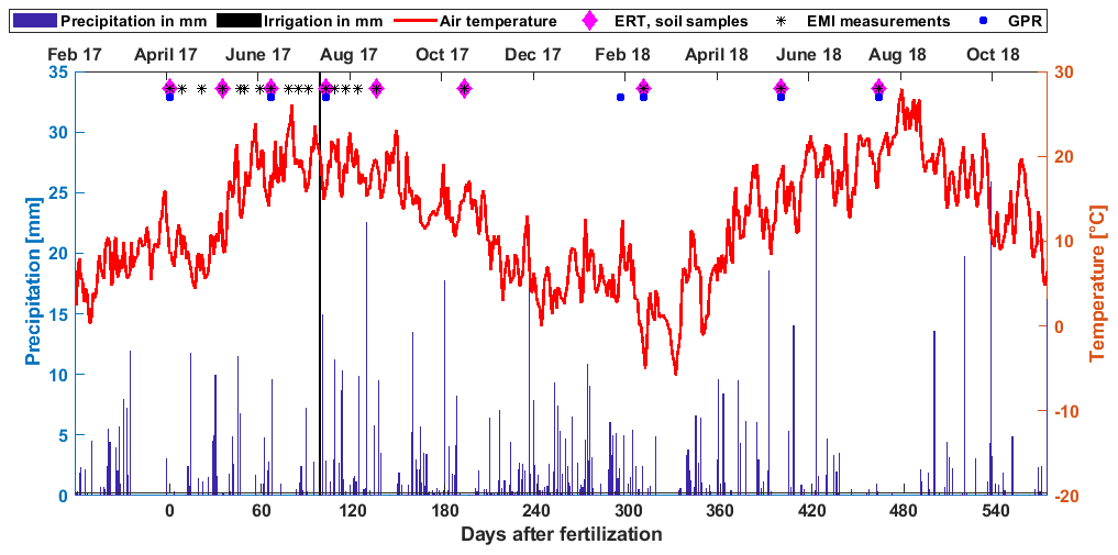
Figure 3 Daily precipitation and daily mean air temperature measured by TERENO climate station SE_BDK_002. The EMI, GPR, and ERT measurement and ground-truth sampling are indicated by pink squares, black stars, and blue boxes, respectively.

2.3 Climate data

Air temperature and precipitation directly affect soil temperature and SWC and, therefore, indirectly affect the geophysical signals measured. Climatic conditions were recorded by the nearby TERENO climate station SE_BK_002 (http://teodoor.icg.kfa-juelich.de, last access: 21 March 2025), located about 50 m south of the experimental plots (see Fig. 1a). For a better illustration, the air temperature is plotted as the daily mean, and the precipitation is provided as the daily sum in millimeters (Fig. 3). Overall, the temperature followed a typical seasonal pattern, with air temperatures ranging from −5 to 30 °C. In the first 90 d, dry weather conditions with low precipitation were observed. To accelerate the downward leaching of the fertilizers, an additional irrigation of 39 mm was applied on 10 July 2017 (DAF 98, highlighted in black). After the irrigation, precipitation increased and remained normal until summer 2018 (DAF 430).

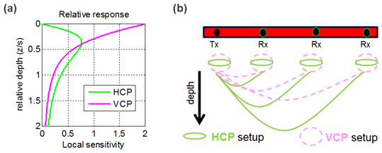
Figure 4 (a) Sensitivity response function after McNeill (1980) for the VCP and HCP EMI configurations, with relative depth normalized by the coil separation. (b) Sketch of a multi-coil MiniExplorer instrument, housing one transmitter and three receiver coils.

2.4 Geophysical data acquisition and data processing

2.4.1 Electromagnetic induction (EMI)

EMI measures the apparent electrical conductivity ECa as a weighted average value over the vertical bulk electrical conductivity distribution within a certain depth volume (Keller and Frischknecht, 1966). The weight average per depth (Fig. 4a), depends mainly on the coil separation s and orientation (McNeill, 1996). Coils can be either oriented vertical co-planar (VCP), which results in more sensitivity to shallow soil depths, or horizontal co-planar (HCP) resulting in increased sensitivity at greater depths (Fig. 4b). The so-called depth of investigation (DOI) is defined as the depth interval in which up to 70 % of the relative response function accumulates. For the VCP and the HCP, this is at around 0.75 and 1.5 times s, respectively (McNeill, 1980). By investigating the relative sensitivity curves for VCP and HCP orientation normalized to the coil separation s, it is clear that the VCP mode is most sensitive to the shallow surface and becomes less sensitive with increasing depth. In contrast, the HCP mode is less sensitive to shallow surface and peaks at a depth of around 0.4 times the coil separation s (Fig. 4a).

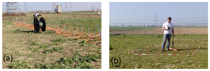
Figure 5 (a) ERT setup of one transects across seven plots and (b) EMI point measurement at one of the treatment plots.

The EMI measurements were carried out with a rigid-boom multi-configuration CMD-MiniExplorer (GF Instruments, Brno, Czech Republic) mounted on a crutch. This system measures with 30 kHz and has three receiver coils (s = 0.32, 0.71, and 1.18 m) and was used in VCP and HCP configuration. The depth of investigation ranged from 0–25 up to 0–118 cm. On all measurement days, the 21 plots were measured four times at different locations within the plots to exclude potential small heterogeneities within a plot. Therefore, the instrument was rotated by 45° horizontally around the plot center (see Fig. 5b). Each measurement was averaged over 100 readings while keeping the instrument stationary and directly on the surface (Fig. 5b). All EMI data were processed with custom-made MATLAB codes. As raw EMI measurements are often prone to systematic errors (e.g., Gebbers et al., 2009; Nüsch et al., 2010), the raw ECa^EMI values were only used for qualitative analyses over time for the same configuration.

2.4.2 Electrical resistivity tomography (ERT)

ERT measures the soil electrical resistivity using galvanic coupling. While, at two electrodes, the current is injected into the ground, the electrical potential difference is measured between two other electrodes. The measured apparent resistivity is an average resistivity over a certain depth and space, depending on the electrode spacing used for the measurement. By measuring different combinations along a transect and following data inversion, a 2D profile of the soil resistivity can be achieved (Binley et al., 2015). In this study, the ERT data were converted to their reciprocal soil electrical conductivity for final analysis and plotting.

The ERT measurements were carried out on nine dates along the same two transects as used for the GPR measurements (see Fig. 2). Therefore, two 30 m long transects were acquired using an electrode spacing of 25 cm and a dipole–dipole setup. Measurements were recorded by a Syscal Pro ERT system (IRIS Instruments, Orlean, France) (see Fig. 5a). Measured data were inverted using the open-access software BERT (https://www.pygimli.org/, last access: 1 December 2018, Rücker et. al, 2017) with a predefined mesh.

2.4.3 Ground-penetrating radar (GPR)

GPR emits electromagnetic (EM) waves, which are reflected or refracted in the soil with changes in either the soil dielectric permittivity or the electrical conductivity. The dielectric permittivity and electrical conductivity can be related to the propagation and the attenuation of the EM wave, respectively. As the fertilizer increases the electrical conductivity of the subsurface, it is expected that we would see differences in the GPR-measured signal attenuation and amplitudes. One common GPR measurement setup is the common-offset profiling (COP), where transmitter and receiver antennae are moved along defined profiles with a constant spacing between the antennae. This method allows us to identify structures in the subsurface. To convert the data measured in time to depth, the measured profiles can be time-to-depth corrected with literature values or point measurements (Jol, 2009).

On 7 different days (see Fig. 3), two transects spanning plot 1 to 7 and plot 15 to 21 (see Fig. 2) were measured with 500 MHz pulseEKKO GPR antennas from Sensors & Software Inc. (Mississauga, Canada). The 30 m long profiles were measured with a common offset of 0.23 m between the transmitter and the receiver. The data are standardly processed (dewow applied, time zero correction, and gain); cut at 1 m depth; and, as an additional step, Hilbert envelope transformed to better visualize amplitude and, hence, electrical conductivity changes. More details about the GPR post-processing can be found in Dal Bo et al. (2019).

2.4.4 Temperature correction of EMI and ERT data

To account for temperature effects on the electrical conductivity and to compare the measurements over time, inverted ERT (EC^ERT) and EMI (ECa^EMI) data were standardized to a reference soil temperature of 25 °C using the approach of Corwin and Lesch (2005):

$$\begin{array}{}\text{(1)}& {\mathrm{EC}}_{\mathrm{25}}={\mathrm{EC}}_{\mathrm{T}}\cdot \left(\mathrm{0.4470}+\mathrm{1.4034}{e}^{(-T/\mathrm{26.815})}\right),\end{array}$$

where EC_T is the electrical conductivity measured at a particular soil temperature T in °C. In our case, the soil temperature of the in situ sensors was used, while the temperature at 60 cm depth was assumed to be valid for deeper depths too. For the ECa^EMI values, the soil temperature was a weighted average based on the depth sensitivity of the EMI configuration (Blanchy et al., 2020).

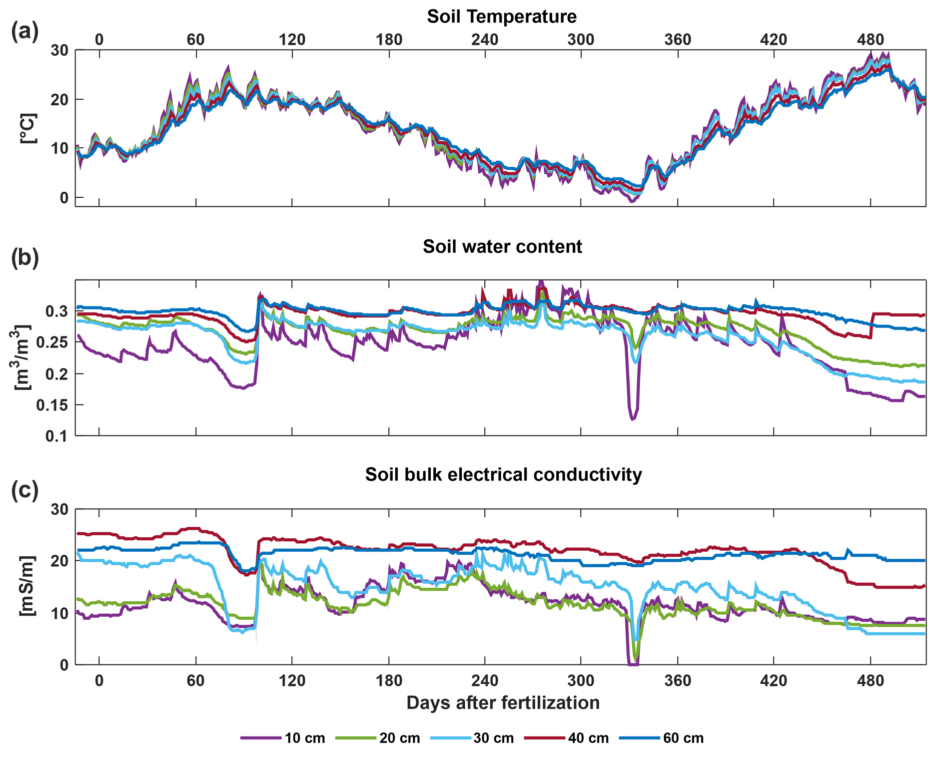
Figure 6 Daily mean (a) soil temperature [°C], (b) volumetric soil water content [m³ m⁻³], and (c) soil temperature corrected (25 °C) soil bulk electrical conductivity ECe^ref [mS m⁻¹] for the depths 10, 20, 30, 40, and 60 cm.

2.5 Soil sampling and chemical analysis

For validation purposes, soil samples were collected over the time of the experiment on the same dates as the ERT and GPR measurements were conducted, resulting in nine ground-truth sampling days (see Table 1). The samples were extracted with a Pürckhauer auger to a maximum depth of 100 cm. The soil cores were divided into predefined depth intervals of 0–10, 10–20, 20–30, 30–40, 40–60, 60–80, and 80–100 cm. The soil was stored in plastic bags at a temperature of 4 °C and then was dried for 48 h at 105 °C and homogenized. The ${\mathrm{EC}}_{\mathrm{e}}^{\mathrm{soil}}$ was measured with a mixture of one part soil and five parts distilled water. Note that the obtained ${\mathrm{EC}}_{\mathrm{e}}^{\mathrm{soil}}$ values are already temperature corrected. Nitrate content (${\mathrm{NO}}_{\mathrm{3}}^{-}$ [mg kg⁻¹]) was measured photometrical according to DIN 38405-9 (Deutsches Institut für Normung, 2011) based on a mixture of one part soil to three parts distilled water. The photometrically measured liquid concentration was back-calculated to the weight of the extracted soil and normalized to $\mathrm{mg}{\mathrm{NO}}_{\mathrm{3}}^{-}{\mathrm{kg}}^{-\mathrm{1}}$ soil. The nitrate concentration was only measured for plots where nitrate fertilizer has been added, and, due to the expected slow vertical translocation of the fertilizer after application only, the shallow samples were measured on the first sampling dates.

2.6 Statistical analysis

All obtained nitrate contents and ${\mathrm{EC}}_{\mathrm{e}}^{\mathrm{soil}}$, ECa^EMI, and EC^ERT data were assigned to the corresponding plot number and DAF. For the ERT data, the inverted conductivity was extracted from the profiles for each plot and depth interval (same depth interval as soil samples). For this, the ERT data were extracted from the profile data over the defined sampling intervals. For the EMI data, measurements in both VCP and HCP mode were considered. As a first analysis step, it was checked if the seven treatments differed significantly compared to the control for each individual measurement day using a Mann–Whitney U test, with a Kruskal–Wallis H test to identify significant differences between means at a probability of p < 0.05. Additionally, the mean (μ) and standard deviation (σ) per plot were calculated, and, out of this, the coefficient of variation (CV; CV = $\mathit{\sigma }/\mathit{\mu }$) was calculated to check the variation within the treatments. The Pearson correlation coefficient r was used to describe the correlation between soil characteristics and geophysical values. The tables corresponding to the statistical analysis can be found in the Supplement.

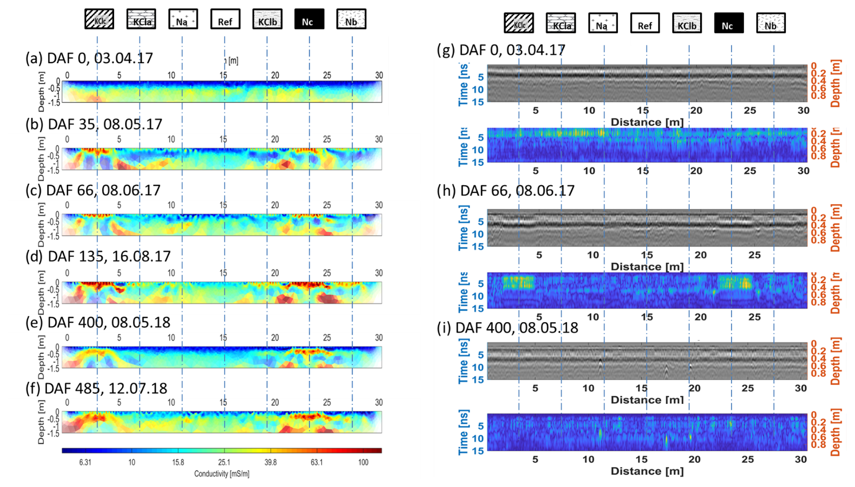
Figure 7 (a–f) Selected inverted ERT profiles (not temperature corrected) showing the effect of fertilization over time on the EC^ERT values. The location of the different plots is indicated at the top of the figure (see Fig. 2 for more information). (g–i) GPR common offset profiling (COP) data for selected dates. The top pictures in the right row show the radargrams, where high and low amplitudes are indicated by white and black colors. Below are the corresponding Hilbert envelope images of the same measurement day.

3 Results and discussion

3.1 Soil sensor data

The soil temperature follows the typical seasonal pattern over all depths (see Fig. 6a). At the start of the experiment, SWC (see Fig. 6b) was in the range of 0.26 to 0.29 m³ m⁻³, but, as a consequence of low rainfall and warm weather conditions, the soil dried out subsequently, and SWC decreased to 0.21 m³ m⁻³ at 10 cm depth on DAF 60–85. After irrigation on 10 July 2017 (DAF 98), SWC at all depths rapidly increased and remained relatively stable until DAF 420. As can be seen, most dynamics were in the shallow sensors (10–30 cm) measuring small fluctuation caused by rain events and dry downs, but a large drop around DAF 330 is also detectable, which is associated with snow coverage in the field. Because of the heatwave in summer 2018, SWC decreased from DAF 420 until the end of the experiment. The soil dried out the most at shallow depths, with a minimum SWC of 0.16 m³ m⁻³.

The ECe^ref showed similar behavior compared to the SWC sensor data, including the decrease during the two drought periods. The two deeper sensors (40 and 50 cm) remained almost stable between 20–25 mS m⁻¹ throughout the entire year. Note that the sensors were installed outside the plot experiments and, therefore, only reflect the EC situation of the control plots.

3.2 Geophysical measurements

3.2.1 Changes across treatments

In a first step, we compare the measured GPR and ERT data across the different treatments exemplarily for transect 2 (see Fig. 2). Before the application of the fertilizers (DAF 0), a relatively homogeneous subsurface with two layers can be identified for both the ERT and GPR data, as shown in Fig. 7a and g, which agrees well with the EMI mapping, which was performed prior to the plot setup (Fig. 1b and c).

In the ERT transect, a low-conductivity layer of 5–10 mS m⁻¹ up to a maximum depth of 50 cm overlying an intermediate EC layer with small internal variation can be observed. The shallow low-electrical-conductivity layer can be associated with the plough horizon, which normally has a lower porosity as the underlying layer (Jeřábek et al., 2017). After fertilization, a clear change in the EC^ERT values across the transect is detectable (Fig. 7b). As expected, the largest changes can be observed for the plots with the highest dosage (the 10-fold dosage of N and KC1 – treatments N_c and KCl_c) applied. The ERT images at DAF 35, 66, and 135 showed an increase in EC^ERT of up to 100 mS m⁻¹ up to a depth of approximately 40 cm (Fig. 7b–d). Over time, the higher EC^ERT values move downward and reached a depth of 100 cm on DAF 485, with an EC^ERT of about 60 mS m⁻¹ (Fig. 7e and f). In contrast, the low dosages (normal recommended N dosage) of N and KCl (KCl_a and N_a) showed only minor changes over time in the ERT-derived EC, while the doubled dosages (KCl_b and N_b) indicate changes in EC^ERT until DAF 135 at shallow depths; furthermore, at later times, the values are smeared over the depth, and no clear effect is optically visible. The reference plot remained relatively stable over time and showed only minor changes, which are mainly related to changes in SWC as a result of precipitation and evaporation.

In the GPR profile gathered before fertilizer application (Fig. 7g), a homogeneous subsurface can also be seen, although small variation in the envelope amplitude in the first 5 ns can be detected. Here, it has to be noted that the GPR signal is attenuated fast because of the high clay content of the soil, and, therefore, deeper subsoil information cannot be obtained, and the information is mainly restricted to the first 20 cm of the ground. Nevertheless, changes in the radargram over time can be detected. For example, on DAF 66, a very strong effect of the high fertilization dosage (KCl_c and N_c) can be seen at the location, not only in the GPR radargram but also in the calculated Hilbert envelop images (Fig. 7h). In contrast, on DAF 400 (Fig. 7i), the GPR transect is almost homogenous, as it was before the fertilizer application, indicating that the fertilizers have been leached to deeper zones and cannot be captured by the GPR or that the concentrations have been diluted to such an extent that they were not detectable anymore. Although amplitude changes were detectable for the high fertilizer application dosages, GPR data were not further interpreted as it was found to be difficult to disentangle various effects on the GPR data (e.g., SWC changes) without additional information about those changes and more advanced data processing such as full-waveform inversion (Liu et al., 2018) or multi-offset GPR (Kaufmann et al., 2020).

3.2.2 Spatial and temporal changes at the point scale

For a more detailed analysis, the temperature-corrected EC values based on the EMI and ERT data, as well as the soil samples, were sorted by depth and treatment over time, and all treatment replicates were averaged (arithmetic mean) and are discussed in the following. In Table S1, significant (p < 0.05) differences in terms of the treatments compared to the control are also listed.

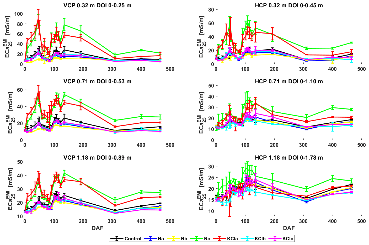
Figure 8 Changes in ECa^EMI over times for the six different EMI configurations; values represent the mean per treatment, and the crossbar indicates the standard deviation. Colors represent the different fertilizer treatments. Note that, for better visualization, different limits in the y axis are used.

EMI measurements

Prior to fertilization on 3 April 2017 (DAF 0), ECa^EMI for the shallowest depth of investigation (VCP 0.32 m DOI = 0–0.25 m) was the lowest at 10.4 mS m⁻¹, and ut was the highest for the deepest configuration (HCP 1.18 m DOI = 1.78 m) at 21.8 mS m⁻¹, indicating a higher SWC in the deeper soil profile (Fig. 8). After fertilization, a clear trend in the measured ECa^EMI can be seen, except for the deepest sensing configuration (HCP 1.18 m), with increased ECa^EMI compared to the control. In particular, the increased ECa^EMI of the higher dosages (b and c treatments) for the two shallow measurement configurations VCP 0.32 m and HCP 0.32 m (DOI = 0.45 m) is quite large, with up to 40 mS m⁻¹. For the deeper configuration and later times, only the high dosages of N and KCl showed elevated ECa^EMI. After fertilization, ECa^EMI increased to its highest values on DAF 49, with a noticeable drop afterwards, explainable by the low SWC and corresponding lower soil bulk electrical conductivity (${\mathrm{EC}}_{\mathrm{e}}^{\mathrm{soil}}$), as shown in Fig. 6c. After the irrigation and precipitation, ECa^EMI increased again and remained high until DAF 195. A smaller drop in ECa^EMI can be observed on DAF 310 for VCP 0.32; HCP 0.32; and, to a lesser extent, VCP 0.71, whereby this drop is earlier in time compared to the sharp drop in SWC and ${\mathrm{EC}}_{\mathrm{e}}^{\mathrm{soil}}$ as found in the sensor data depicted in Fig. 6c. A more detailed examination of the sensor data reveals a slight decline in SWC at a depth of 20 cm, which appears to be linked to a brief period of reduced SWC and a corresponding decrease in electrical conductivity in ECa^EMI.

Over the complete time span, the coefficient of variance was, for all treatments and configurations, except for a few outliers, below 0.4, whereby, for the smallest coil configuration (VCP and HCP 0.32), in general, more spread (between 0.2 and 0.4) is present than in the other configurations (mainly below 0.2). Additionally, for ECa^EMI, significance in terms of the differences between the treatments and the control was calculated, and it can be seen that ECa^EMI for the normal dosage (N_a) never differed significantly from the control. In contrast, for KCl_a, low significant differences (p > 0.2) were present between DAF 20 and 135, except for the days with low SWC (DAF 66–91) for the VCP configuration. Additionally, in the double-dosage treatment (b), significantly higher differences can be observed within the KCl_b treatment compared to for N_b. Hereby, N_b is mainly significantly different compared to the control at p < 0.05, whereas, for KCl_b, it is mainly different at p < 0.01 after DAF 35 and until DAF 193 for all three VCP configurations and for HCP 0.32 and HCP 0.71. Only the dates between DAF 66 to 91 for the double treatment (N_b) are not significantly different from the control, with those dates being associated with low SWC in the shallow soil. In contrast, plots treated with KCl_b are less affected by the SWC drop and were still significantly different compared to the control. For the deepest sensing configuration, HCP 1.18, no significant difference was measured at any time of the experiment. The highest dosage (N_c and KCl_c) differed significantly (p < 0.01) for all three VCP configurations and for HCP 0.32. For HCP 0.71, high to medium significant (p < 0.5) differences compared to the control were found, except for DAF 66 for KCl_c, whereas the deepest sensing configuration, HCP 1.18, only started to differ significantly after DAF 102 (except for DAF 135) for N_c and after DAF 310 for KCl_c. This pattern indicates that the fertilizer slowly moved downwards over time. This analysis used non-calibrated EMI data because they are classically available and are the easiest and fastest to be acquired. However, such EMI data cannot be used to invert depth-specific bulk EC, which could improve the analysis.

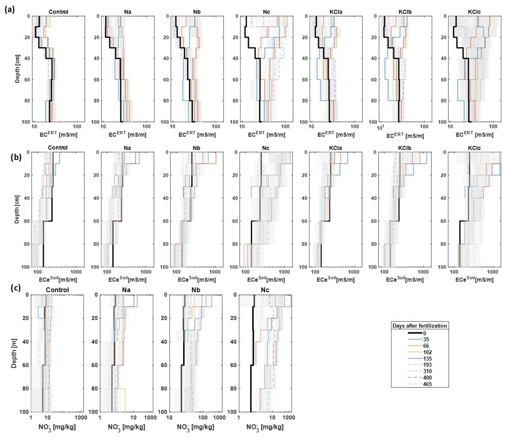
Figure 9 Comparison of the mean (a) EC^ERT [mS m⁻¹], (b) ${\mathrm{EC}}_{\mathrm{e}}^{\mathrm{soil}}$ [mS m⁻¹], and (c) nitrate concentration [mg kg⁻¹] for each treatment over time. As the reference, the depth profile prior to fertilization is shown in black. The gray color indicates the standard deviation. Note that the x axis scale is logarithmic for better visualization.

ERT measurements

In comparison to the non-calibrated and non-inverted EMI data, depth-specific data can be obtained for the ERT as shown in Fig. 7 for the intervals 0–10, 10–20, 20–30, 30–60, 60–80, and 80–100 cm. Overall, the ERT-derived electrical conductivity followed a similar trend to the EMI data, especially for both high dosages (N_c and KCl_c) applied, whereby one can notice that EC^ERT is mostly affected by the fertilization application in the top layers over all sampling dates. It is also clearly visible that the downward movement of the fertilizers over time can be detected and can be easily followed for the high dosage (N_c), where EC^ERT was highest for early measurement days in the top layer up to a depth of 30 cm, whereas, for the later measurement days (DAF 310 and after), EC^ERT was higher for the layer 10–20 cm compared to that measured for the first layer (0–10 cm). Note that the control plot did show smaller changes in measured EC^ERT over time, with these changes only being caused by changes in SWC. Even though the daily covariance was relatively low (> 0.4, except for a few outliers) over the course of the experiment, for the highest dosage (N_c and KCl_c), the largest spread in EC data over depth can be observed. Also, for EC^ERT, significance in terms of the differences between the treatments and the control was observed. For the normal dosage (N_a) only a few significant (p < 0.05) differences were present directly after the fertilization application on DAF 8 at a depth between 20–40 cm and between 80–100 cm. For the deeper depth, a significant difference was found for DAF 102–193. For N_b, KCl_a, and KCl_b, similar patterns were observed, with highly significant differences at shallow depths (0–10 cm) on DAF 36; at 10–40 cm from DAF 36 to DAF 193, except on DAF 66 at a depth of 40 cm; and at 60–100 cm between DAF 102 and 193. After DAF 193, no significant difference compared to the control was found for the normal and double dosages (except at 10 cm on DAF 193 for N_b). For the highest dosage (N_c and KCl_c), for depths between 30–100 m, highly significant differences (p < 0.01) with respect to the control were observed from DAF 36 until the end of experiment (DAF 485); for the shallow depth (0–20 cm), no significant difference was found on DAF 310 and 400. However, for DAF 410 and 465, significant differences were present again for the application with the 10-fold dosage.

Similarly to the EMI results, the ERT data showed downward leaching of the fertilization over time, but this was better depth resolved compared to the data obtained by means of EMI. This result is to be expected as ERT is capable of vertically resolving EC differences with high spatial resolutions and with low EC differences, as stated by Garré et al. (2011). In contrast, for the normal and double dosages, the fertilizer leached deeper than 20 cm within the first 2 months, leading to dispersion of the masses and concentrations (Ellsworth and Jury, 1991) and, therefore, also to lower impacts on the gathered geophysical signals. As a consequence of further translocation, spreading of the fertilizer plume and the difference compared to the control became statistically irrelevant (similarly to that which is shown for the EMI results). However, this also showed that normal fertilization rates clearly impact geophysical measurements, at least at a certain time after application. Therefore, this effect should not be neglected if geophysical measurements are performed over different fields not managed the same way; if different areas within a single field are fertilized differently; or if plants take up different amounts of fertilizer due to variable plant growth induced by, e.g., non-homogeneous water supply. Finally, we can conclude that both EMI and ERT measurements showed fewer differences between the treatments and the control on days with low SWC (for example, DAF 66 or 193), which is in line with previous findings by Schmäck et al. (2022). As a consequence, this means that optimal SWC conditions are required for EMI and ERT surveys to identify differences in fertilization states of the soils, whereby the most suitable are conditions with relatively high SWC values.

Soil nitrate concentrations and soil bulk electrical conductivity

For further interpretation of the geophysically derived information, the nitrate concentrations and ECe^soil data for the soil samples analyzed in the laboratory were investigated (Fig. 9b and c). As the nitrate analysis is time consuming, only those depths where elevated nitrate concentrations were measured in the preceding measurement days and the next underlying sampling layer were analyzed. If the next layer also showed higher concentrations compared to the reference (with the reference equating to the concentration prior to fertilizer application), the next depth was also analyzed. This simplification can be made if preferential water flow and the associated preferential solute transport can be excluded and if only slow matric flow of the solutes is assumed. For those layers not analyzed for the corresponding sampling day, the nitrate concentration measured prior to fertilizer application (DAF 0) was considered. KCl was also not measured as the extraction and measurements are also extremely tedious and costly, and the overall focus of the study was on N fertilization effects.

Overall, the ECe^soil and nitrate concentrations followed a similar trend as the EMI or ERT data, especially for both high dosages of N and KCl (Fig. 9). The mean ECe^soil in the control plot varied to a small extent between 3 and 15 mS m⁻¹ in the first 20 cm over time, probably affected by weather events and translocation of the background solute and/or mineralization of organic matter (Fig. 9b). At greater depths, ECe^soil decreased to values round 8 mS m⁻¹, likely caused by a lower organic matter content and, therefore, lower release of DOC. The mean soil nitrate concentrations in the control plot also varied to a small extent between 5 and 15 mg ${\mathrm{NO}}_{\mathrm{3}}^{-}$ kg⁻¹ soil, with some variability over the nine measurement dates (see Fig. 9c) likely caused by small-scale heterogeneity of the soil and the small-scale sampling via the Pürckhauer auger (see detailed discussion below). In general, the nitrate concentrations in the upper 60 cm of the control plots were always slightly higher than those in the deeper soil, which can be attributed to the lower organic matter content at greater depths, forming less nitrate by decomposition. As already discussed for ECe^soil, the temporal changes in the nitrate concentration of the control plot, where no N fertilizer was applied, can be probably associated with the mineralization of organic matter as stimulated by higher soil temperatures in the uppermost centimeters of the soil profile and with nitrate release into the soil.

As expected, the highest ECe^soil and nitrate concentrations were found in the high-dosage plots (N_c and KL_c). In general, ECe^soil followed a similar pattern to that discussed for EC^ERT. Looking at the nitrate concentrations, we can notice that the nitrate concentrations increased rapidly after the fertilizer application up to approximately 1400 mg kg⁻¹ in the first 10 cm until DAF 66 for the high dosage (Fig. 9c). After irrigation and further precipitation, the nitrate concentrations decreased in the upper 10 cm but still remained higher than those found in the control plot. Despite the high values found, no significant differences (p < 0.2) were observed for any depth or treatment for the normal and double dosages for ECe^soil and nitrate content with respect to the control plots. For the high dosage, a significant difference (p < 0.1) was partly present for ECe^soil at 0–10 cm on DAF 102 and 195, for KCl_c on DAF 36 and 193 at a depth of 10–40 cm, and for N_c and KCl_c from DAF 102 to 400 (except DAF on 310 at 10–20 cm depth for N_c). For 80–100 cm depth, the N_c treatment differed significantly from the control on DAF 310–465, and the KCl_c treatment differed significantly from the control on DAF 102 and from DAF 310 to 465. For the nitrate content of the N-fertilized plots, similar patterns as for ECe^soil can be observed, with the highest concentrations for the highest dosages, especially for the shallow depth, over the entire experimental period and a slow downward movement over time. Interestingly, higher concentrations are also found in the highest-dosage plots (N_c) at later times, indicating a downward movement of the nitrate.

In general, the soil sample data ECe^soil and the nitrate concentrations had the highest CV of all measurements, which explains the weaker significant differences between the treatments and control compared to ERT and EMI, which both showed lower CV. The high variability of the nitrate concentrations and ECe^soil of the soil samples can be partly explained by the sampling itself – as only a few soil samples were extracted (one per plot, with three per treatment) compared to EMI (4 per plot, with 12 per treatment) and ERT (∼ 5 per plot, with 10 per treatment) – and by the small volume sampled by the Pürckhauer auger. For EC^ERT on DAF 310 and beyond, we speculated that the decrease in EC^ERT is caused by downward movement of the nitrate to deeper soil layers. Looking at the ECe^soil data and nitrate concentrations, we can see the same pattern of lower ECe^soil values in the upper soil layer (0–10 cm) and higher ones in the underlying layer. The same holds for the nitrate concentrations. As ECe^soil and the soil nitrate concentrations are independent of the SWC changes, this only showed the actual status of ions available at a certain time in the soil and, therefore, proved the hypothesis of downward translocation.

Table 2 Pearson correlation coefficients (r) between ECa^EMI (VCP and HCP), EC^ERT, and ECe^soil with the measured (a) nitrate concentrations and (b) SWC data from the sensors for depths (d) between 10 to 120 cm. Note that the mean values gathered over all plots within the same treatments for each measurement day have been used. Correlation was style coded according to r, with high correlation coefficients in bold and underlined (r > 0.8), moderate correlations in bold (0.5 < r > 0.8), low correlations in normal roman font (0.3 < r > 0.5), and no correlation in italics (r < 0.3). The definitions of the quality of the correlation coefficients r are similar to those defined by Schmäck et al. (2022).

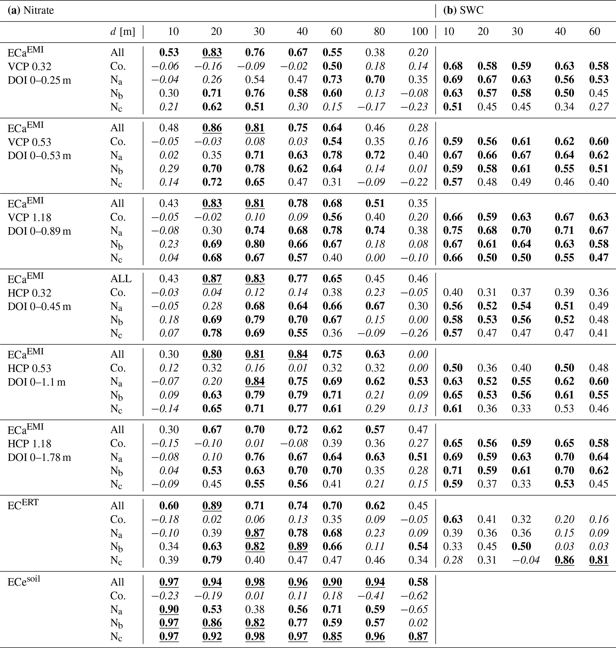
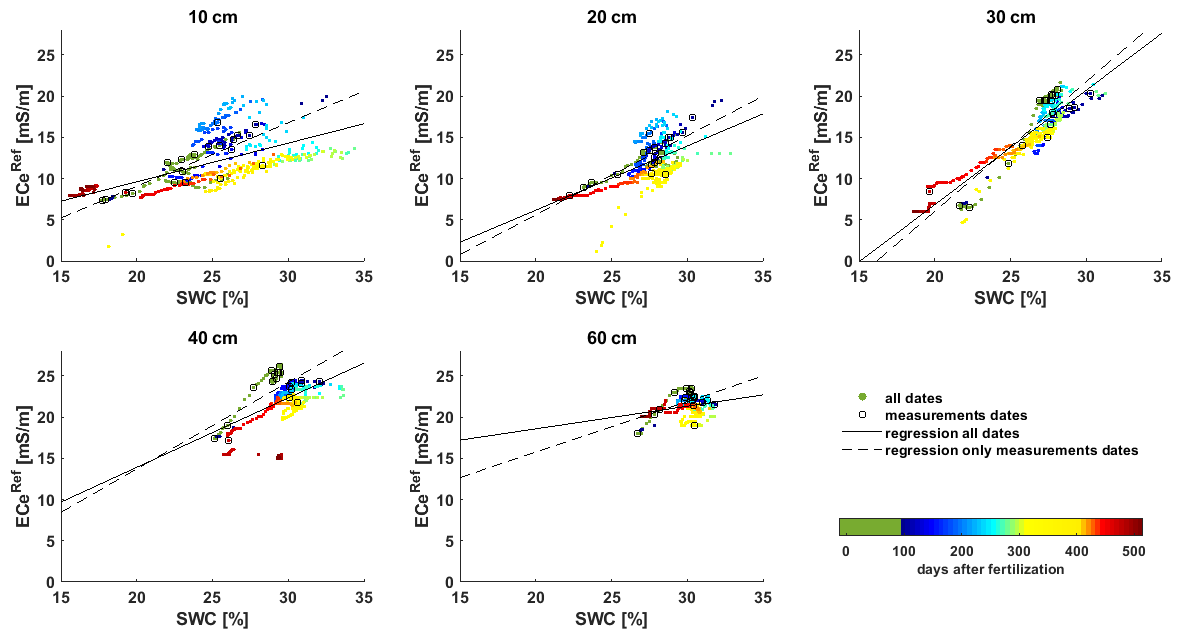
Figure 10 Linear regression between ${\mathrm{EC}}_{\mathrm{e}}^{\mathrm{ref}}$ and SWC measured by the soil sensors over all 485 d of the experiment. The color indicates the day after fertilization. The values of the main measurement day are highlighted, indicating the time after the fertilization (green points prior to irrigation).

3.2.3 Correlation between measured soil states

Generally, geophysical measurements such as those gathered by EMI and ERT are influenced by various soil states and parameters such as soil texture (e.g., clay content), soil pore water salinity, and soil temperature (McNeill, 1980; Corwin and Lesch, 2005). Therefore, one aim of this study was to disentangle the impact of fertilization on the measurement signal. Therefore, correlations between the different measured states were performed (Table 2 and Tables S1–S4). As the soil texture will not affect the results measured in the different treatments due to the fact that soil texture is known to be very stable over time (Upadhyay and Raghubanshi, 2020), soil texture can be assumed to be a static component in the analysis and, therefore, can be neglected.

In a first step, the sensor-based SWC and ECe^ref of the sensor data were correlated (Fig. 10). Note that the correlation was performed either for the entire dataset measured over the entire period or for the single days where geophysical measurements were acquired. Before looking into the details of the individual correlations, attention should be drawn to the effect of irrigation on ECe^ref. Directly after the irrigation (blue dots in Fig. 10) on DAF 98, ECe^ref showed higher values for respective SWCs and dropped down to lower ones for the same SWCs (yellow to red dots). This effect can be explained by the higher electrical conductivity of the irrigation water used (49.1 mS m⁻¹) compared to the rainwater (classically between 3–6 mS m⁻¹ in the region) feeding the soil water under non-irrigated conditions. As shown by Kaufmann et al. (2019), the irrigation does not only affect the soil EC over short times but can be traced back by EC measurements over longer periods. However, at a deeper depth (30–60 cm), ECe^ref was less affected by the irrigation as the irrigation water had to travel downwards and also had to mix with already existing pore water and, thereby, had to be equilibrated in relation to the ion concentration.

Coming back to the correlation (Fig. 10), it becomes visible that, for the shallow subsurface between 0–30 cm depth, a moderate correlation for both the entire dataset and measurement days (r > 0.6) was calculated, whereby the effect of the irrigation becomes less and less pronounced in the deeper soil layers as the points (bluish and red or yellow) get closer to each other. For depths of 40 cm, the correlation over all days is slightly lower (r = 0.43), and, at 60 cm, only a low correlation (r = 0.25) for the entire dataset was found. The low correlation, especially at 60 cm depth, can be explained by the low variability of ECe^ref and SWC. Considering only the days where geophysical measurements were performed, the correlation generally increased for all depths and exceeded r values of 0.8 for the depths of 10 to 30 cm. Even at lower depths, r stayed relatively high, with r = 0.7 and 0.51 for 40 and 60 cm depth, respectively.

As the next step, the impacts of the confounding factors SWC or nitrate concentration on the geophysical measurements were analyzed. Therefore, the ECa^EMI of all six coil configurations, EC^ERT, and the reference lab-derived ECe^Soil were correlated with the nitrate concentrations sampled and SWC gathered by the sensors per treatment (Table 2). The correlations with parameters per plot (soil vs. geophysics) are additionally found for all treatments together. The definitions of the quality of the correlation coefficients r are based on those suggested by Schmäck et al. (2022), whereby Schmäck et al. (2022) used R² values instead of Pearson's r. In general, for both EMI and ERT data, the combined correlation, where all data from all treatments were used together, with nitrate content and ECe^soil had a high to moderate correlation (r > 0.4) for the N-fertilized plots. The low correlation for the control plot might be explained by the general low variability in the data (see Fig. 9) but also clearly shows that all observed effects are mainly related to the fertilization and not to changes in other soil states. The low correlation for the shallow soil layer (0–10 cm) over all EMI configurations and also, partly, for ERT is somehow surprising as, especially in this layer, the most variation in nitrate concentration over time was observed (Fig. 9). As ECe^soil versus nitrate showed the highest correlation, not only over the entire profile but also for the shallow layer of 0–10 cm, except for the control, this shows that the geophysical sensors used (ERT and EMI) are less suited to gathering information from the very shallow soil up to 10 cm. For ERT, an electrode spacing of 0.25 cm was used, resulting in 1 m coverage of the four electrodes used for one single measurement (thus being partly influenced outside of the plots). Reducing the electrode spacing is theoretically feasible, as shown by Ochs and Klitzsch (2020), but would lead to lower depths one can investigate and lower resolutions at larger depths. Additionally, spatial smoothing is applied in the standard inversion used, limiting the small-scale resolution, as shown by Kemna et al. (2002). The EMI-derived ECa values are a weighted depth function of the retrieved signal, and so, laterally, one measurement spans at least the coil separation and the depth resolution. The sensitivity of the EMI configuration spans the soil sample interval and is therefore affected by different depths. Therefore, we can conclude that the shallow ECa^EMI seems to be additionally affected by other soil states and, therefore, is not suitable to measure the effect of fertilization in those shallow soil layers.

As generally known and as shown in Fig. 10, SWC has a large impact on the soil electrical conductivity, ECe^ref, measured by the sensors installed in the soil profile. Therefore, we also analyzed the impact of SWC on measured ECa^EMI and EC^ERT by correlating the sensor-based SWCs measured on the days of geophysical measurements against ECa^EMI and EC^ERT assuming that SWCs are the same in all plots as those measured at the reference location. As can be seen in Table 2, the correlation is much better if we look at all depths and EMI configurations used compared to the correlation of ECa^EMI with N. Additionally, the shallow soil depth 0–10 cm showed better correlations now. Only for the correlation between EC^ERT and SWC cab no clear improvement be detected, and one can even find a slightly worse correlation between the two states. In contrast, high correlations (as indicated with the solid bold black in Table 2) do not show up for the correlation with SWC at all. Additionally, one can detect that the correlation is, in most cases, weaker for the high fertilizer application (N_c) compared to lower dosages applied, which corresponds to the higher correlation found for the high nitrate concentrations (N_c) and electrical conductivity, as discussed before. This means that SWC has an overall impact on the measured EC at all fertilization levels, but at high fertilization rates, the nitrate impacts the measured EC to a larger extend. Finally, the question arises of why the shallow soil layers (0–10 cm) were better correlated to SWC compared to nitrate concentration. On the one hand, SWCs were all measured at one location (sensor pit) ignoring local soil heterogeneities, whereas the correlation with nitrate concentrations is based on two measurements within the same plot. Potentially the high variability (as expressed in high coefficient of variation) of the nitrate concentration might affected the correlation between nitrate and the geophysical measurements. Additionally, looking at the temporal course of EC^EMI data (Fig. 8), it was observed that at days with low SWC the measured electrical conductivity dropped (e.g., around DAF 66 or 310), whereas the corresponding nitrate concentration dropped to a smaller extent as the nitrate mass per soil volume is not directly connected to the mass of water in the same soil volume. Nevertheless, the pore water conductivity must increase if nitrate masses stay unaffected, but SWC drops. This leads to the conclusion that, at low SWC content, the EMI and ERT methods seem not to be appropriate to detect changes in nitrate concentrations.

Based on the correlation between the obtained electrical conductivities and depth-dependent nitrate concentrations, especially over all treatments, one can conclude that high nitrate levels can be measured with moderate to higher accuracy in the clay soil studied. This also means that large differences in the nitrate level between fields or within fields might lead to differences in gathered ECa^EMI. This fact can either support the delineation of inner-field management zones or complicate the explanation of “jumps” in measured ECa^EMI across field boarders, even if the same crop has been grown. That nitrate differences in the soil can be measured by EMI has been already shown by Eigenberg et al. (2002) and Eigenberg and Nienaber (2003). In contrast to the work presented here, both the aforementioned studies did not only add nitrate to the soil but also analyzed situations that are more complex. In Eigenberg et al. (2002), a 7-year manure and cover crop experiment was analyzed, where both the manure and the cover crops impact soil organic matter content soil structure, and water retention and, therefore, measured ECa^EMI. In the second study, Eigenberg and Nienaber (2003) studied the impact of compost piles on measured ECa^EMI, but, also, here, various changes in the soil (higher SOC, retention capacity, etc.) might have affected the signal and not only nitrate stock differences.

4 Summary and conclusion

In the study presented, time-lapse geophysical measurements using EMI, ERT, and GPR were used to analyze the impact of fertilization on the measured geophysical signals. Therefore, two different fertilizers (calcium ammonium nitrate and potassium chloride ) were applied at three different dosages to field plots in triplicate. Although the GPR data could not be used for a detailed analysis because of the high attenuations of the EM waves, for other soil types, where the background electrical bulk conductivity is smaller, GPR could help to map the SWC distributions in the soil over time. The results of this work showed that ERT was suitable to detect the impact of fertilization on bulk electrical conductivity over the entire course of the experiment (438 d), especially for the case of extremely high fertilizer application (10-fold increase compared to the recommended dosage). EMI was also not able to measure differences between the low fertilizer dosage applied (190 kg N ha⁻¹) and the unfertilized control, but for higher dosages, EMI was able to trace the differences in electrical conductivity over longer time periods. Interestingly, EMI was able to detect KCl with 190 kg ha⁻¹. The correlation between EMI- and ERT-derived electrical conductivities and ground truth nitrate data showed that both techniques failed to trace the fertilizers back in the shallowest soil layer 0–10 cm and were not able to reproduce small changes in nitrate concentrations in the unfertilized control plot. Based on the study, we can conclude that EMI and ERT are suitable for detecting different fertilization levels in a clay soil if the fertilization differences are large enough but fail if concentrations are extremely small, such as those in 10-year-old bare soil without fertilization. Nevertheless, the study showed that the geophysical measurements are suitable for detecting differences in fertilization even over a longer time span of more than 1 year. In addition, we observed that relatively high SWC conditions are the most appropriate conditions in which to identify differences in fertilization states. Based on the findings presented, we recommend not neglecting the past fertilization practices in EMI studies, especially if larger are surveyed with different fertilization practices or crops with different fertilizer demands are surveyed.