An ensemble estimate of Australian soil organic carbon using machine learning and process-based modelling

Spatially explicit prediction of soil organic carbon (SOC) serves as a crucial foundation for effective land management strategies aimed at mitigating soil degradation and assessing carbon sequestration potential. Here, using more than 1000 in situ observations, we trained two machine learning models (a random forest model and a k-means coupled with multiple linear regression model) and one process-based model (the vertically resolved MIcrobial-MIneral Carbon Stabilization, MIMICS, model) to predict the SOC stocks of the top 30 cm of soil in Australia. Parameters of MIMICS were optimised for different site groupings using two distinct approaches: plant functional types (MIMICS-PFT) and the most influential environmental factors (MIMICS-ENV). All models showed good performance with respect to SOC predictions, with an R² value greater than 0.8 during out-of-sample validation, with random forest being the most accurate; moreover, it was found that SOC in forests is more predictable than that in non-forest soils excluding croplands. The performance of continental-scale SOC predictions by MIMICS-ENV is better than that by MIMICS-PFT especially in non-forest soils. Digital maps of terrestrial SOC stocks generated using all of the models showed a similar spatial distribution, with higher values in south-eastern and south-western Australia, but the magnitude of the estimated SOC stocks varied. The mean ensemble estimate of SOC stocks was 30.3 t ha⁻¹, with k-means coupled with multiple linear regression generating the highest estimate (mean SOC stocks of 38.15 t ha⁻¹) and MIMICS-PFT generating the lowest estimate (mean SOC stocks of 24.29 t ha⁻¹). We suggest that enhancing process-based models to incorporate newly identified drivers that significantly influence SOC variation in different environments could be the key to reducing the discrepancies in these estimates. Our findings underscore the considerable uncertainty in SOC estimates derived from different modelling approaches and emphasise the importance of rigorous out-of-sample validation before applying any one approach in Australia.

1 Introduction

Globally, the soil is the largest biogeochemically active terrestrial carbon pool, storing more organic carbon than plants and the atmosphere combined (Jackson et al., 2017). The turnover of soil organic carbon (SOC) is a key function in plant growth, maintenance of soil water and nutrients, soil structure stabilisation, and other biogeochemical processes (Lefèvre et al., 2017). Soil can act as either a carbon sink or carbon source, depending on the balance of carbon input through plant litter and root exudates and output through respiration and leaching (Terrer et al., 2021; Panchal et al., 2022). Even a small change in SOC stocks, in any direction, could significantly affect the atmospheric concentration of CO₂ and, thus, climate change (Stockmann et al., 2013).

Given the importance of SOC, there is now a large and growing interest in estimating the spatially explicit SOC content and stocks. SOC supports critically important soil-derived ecosystem services, and the amount of SOC indicates the degree of land and soil degradation (Lorenz et al., 2019). An SOC content below a certain limit will lead to a decline in microbial diversity, water holding capacity and soil productivity (Stockmann et al., 2015). Additionally, with growing concerns about increasing anthropogenic CO₂ emissions, soil carbon sequestration has emerged as a potential strategy for climate change mitigation (Smith, 2016; Rumpel et al., 2018). The protection of existing SOC and rebuilding depleted stocks through land management are potential strategies for mitigating climate change (Bossio et al., 2020). However, effective SOC management requires accurate knowledge of its existing distribution. Reliable estimates of SOC stocks and their spatial variation serve as a reference point for assessing how close soil is to its maximum SOC storage capacity and its potential to sequester additional carbon (Six et al., 2002; Georgiou et al., 2022). Precise estimation of contemporary SOC stocks also provides a baseline map that can be used to calibrate and initialise dynamic mechanistic models, enabling the study of how SOC will respond to climate and land-use change (Minasny et al., 2013; Viscarra Rossel et al., 2014). It is, for example, a prerequisite for accurately predicting the future carbon–climate feedback in Earth system models (ESMs) (Todd-Brown et al., 2013).

Accurately assessing SOC storage is challenging due to the complexity of carbon formation and degradation processes in space and time (Keskin et al., 2019). Soil exists as a continuum, containing organic compounds at different stages of decomposition (Lehmann and Kleber, 2015). Soil formation can be described by a function of climate, organisms, relief, parent material and time (Jenny, 1941). These factors are widely used in SOC studies for digital soil mapping (McBratney et al., 2003; Viscarra Rossel et al., 2015; Liang et al., 2019). However, the relationship between SOC storage and these driving variables is complex and spatially variable (Mishra and Riley, 2015; Viscarra Rossel et al., 2019; Adhikari et al., 2020), leading to substantial challenges and inherent uncertainties in SOC predictions.

Mechanistic process-based models and empirical models (including machine learning models) are two widely employed approaches used to predict SOC stocks and their spatial distribution. Conventional process-based models assume first-order kinetics for SOC decomposition, wherein the rate of C decomposition is dependent on temperature and moisture but independent of microbial biomass, while the equilibrium SOC stock is proportional to the carbon input and mean residence time (Abs and Ferrière, 2020; Wang et al., 2021). ESMs coupled with conventional SOC models cannot accurately simulate the spatial pattern of contemporary soil carbon and show large divergence in projected SOC dynamics under future climate change (Todd-Brown et al., 2013, 2014). In addition to the biases introduced by errors in model parameters and the lack of independent model validation based on observed time series data, the uncertainties in predicted SOC by ESMs can also result from a lack of the explicit representation of soil microbial activities and metabolic traits (Wieder et al., 2015; Le Neo et al., 2023). Numerous microbial models have been developed in the past few decades to improve the model performance of SOC predictions (Chandel et al., 2023), but these models have rarely been incorporated into large-scale modelling frameworks due to the difficulty involved with constraining parameters relating to microbial activities and the lack of rigorous validation (Todd-Brown et al., 2013; Luo et al., 2016). Process-based SOC models are constructed based on our understanding of the major processes governing SOC dynamics (e.g. carbon input, decomposition and loss). However, the disagreement with respect to the projections of carbon dynamics by different models highlights the need to improve our knowledge of SOC cycling (Luo et al., 2016). Machine learning models without any process-level assumptions provide a tool to identify the most influential controls on SOC variations. Machine learning models can represent non-linear and non-smooth relationships between the predictor and response variables as well as interactions between different predictors (Heung et al., 2016). Various machine learning algorithms have been successfully used in digital soil mapping to predict high-resolution, spatially explicit SOC concentrations or stocks (Lamichhane et al., 2019).

Several modelling studies of soil carbon stocks have been conducted in Australia. Wang et al. (2018a) trained boosted regression trees and random forest models using field observations and applied the trained random forest model to map the spatial distribution of SOC at two soil depths (0–5 and 0–30 cm) for the semi-arid rangelands of eastern Australia. Continentally, Viscarra Rossel et al. (2014) trained the CUBIST model, a form of piecewise linear decision tree, using more than 5000 observations to produce a high-resolution (90 m×90 m) baseline map of the SOC stocks of Australian terrestrial systems and their related uncertainty in the top 30 cm of soils. Based on the baseline map, Walden et al. (2023) derived spatially explicit estimates of Australian SOC stocks and uncertainty that included additional data from forests in south-eastern Australia and coastal marine (or blue-carbon) ecosystems. The SOC content at multiple soil depths and the associated uncertainties were also estimated using different machine learning algorithms (Viscarra Rossel et al., 2015; Wadoux et al., 2023). Moreover, the distribution of different soil carbon compositions (i.e. the particulate, mineral-associated and pyrogenic organic carbon fractions) and the importance of environmental factors on their variations were also studied using machine learning (Viscarra Rossel et al., 2019). However, despite the progress made in SOC modelling, significant uncertainties persist in SOC estimates due to the inherent complexities of SOC variation and the lack of appropriately sampled SOC observations. All of these continental estimates were generated using empirical modelling approaches or first-order biogeochemical models without explicitly representing the important role of soil microbes in SOC stabilisation (Grace et al., 2006; Lee et al., 2021). Estimates from mechanistic SOC models with the explicit representation of microbial metabolism are missing, despite the fact that they offer the potential to better constrain SOC dynamics under future climate change scenarios in a way that empirical approaches cannot.

Our primary objective in this paper is to assess the predictability of the SOC concentration (excluding cropland soils) in Australia; generate a range of estimates of terrestrial SOC stocks, employing both process-based and empirical modelling; and examine why these estimates might differ. First, we discern the significance of environmental predictors, at both continental and biome scales. We then evaluate the performance of random forests, k-means with multiple linear regression and the vertically resolved MIcrobial-MIneral Carbon Stabilization (MIMICS) model with different parameterisation approaches. Finally, we compare the spatial estimates of SOC stocks using these different approaches across Australia and discuss their differences and potential application to future SOC projection.

2 Materials and methods

2.1 Model descriptions

2.1.1 Vertically resolved MIMICS

The MIMICS model (Wieder et al., 2015; Zhang et al., 2020) explicitly considers relationships between litter quality, functional trade-offs in microbial physiology and the physical protection of microbial by-products in forming stable soil organic matter. There are two litter pools – metabolic (LIT_m) and structural (LIT_s) litter (Fig. 1) – and the partitioning of litter input into metabolic and structural pools is determined by the chemical properties of the litter. Litter and SOC turnover are governed by two microbial functional types that exhibit copiotrophic (i.e. r-selected, MIC_r) and oligotrophic (i.e. K-selected, MIC_k) growth strategies. MIC_r is assumed to have higher growth and turnover rates as well as a preference for consuming labile litter (LIT_m), while MIC_k is characterised by lower growth and turnover rates as well as a greater competitive advantage when consuming low-quality litter (LIT_s) and chemically recalcitrant SOC. SOC in MIMICS is divided into three pools: physically protected (SOC_p), (bio)chemically recalcitrant (SOC_c) and available (SOC_a) carbon (Fig. 1).

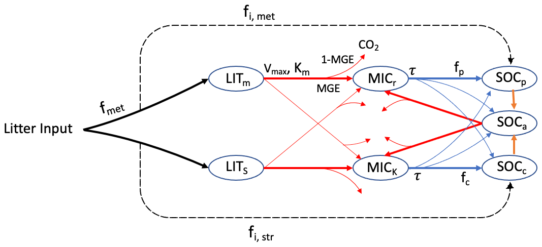
Figure 1 SOC pools and fluxes represented in MIMICS (adapted from Wieder et al., 2015). Litter inputs are partitioned into metabolic and structural litter pools (LIT_m and LIT_s, respectively) based on litter quality (f_met). Decomposition of litter and the available SOC pool (SOC_a) are governed by temperature-sensitive Michaelis–Menten kinetics (V_max, maximum reaction velocity; K_m, half saturation constant), shown by red lines. Microbial growth efficiency (MGE) determines the partitioning of C fluxes entering the microbial biomass pools vs. heterotrophic respiration. Turnover of microbial biomass (τ, blue) depends on microbial functional types (MIC_r and MIC_k) and is partitioned into available, physically protected and chemically recalcitrant SOC pools (SOC_a, SOC_p and SOC_c, respectively).

The decomposition of litter pools and SOC pools follows temperature-sensitive Michaelis–Menten kinetics. Microbial growth efficiency (MGE) determines the partitioning of carbon fluxes entering microbial biomass pools (MIC_r and MIC_k) vs. heterotrophic respiration. Access of microbial enzymes to available substrates depends on the soil texture. The equations of MIMICS are from Wieder et al. (2015), except that the density-dependent microbial turnover was introduced to MIMICS to minimise an unrealistic oscillation (Zhang et al., 2020). To better simulate carbon turnover at different soil depths, the vertical transport of soil carbon was introduced into MIMICS, thereby considering carbon transported through bioturbation and diffusion among adjacent soil layers (Wang et al., 2021).

Vertically resolved MIMICS is run using a daily time step. The soil was divided into 15 layers, each of 10 cm thickness. All of the sites in this study are assumed to be in steady state (i.e. no interannual variation in SOC). Historical climate, litterfall input and soil properties were all assumed to be similar to the average conditions. At each site, the initial pool fractions were 0.03, 0.03, 0.14, 0.47 and 0.33 for MIC_r, MIC_k, SOC_p, SOC_c and SOC_a, respectively. All pools were then spun up to finally achieve steady state, with the maximal difference in any pool size between two successive spins being less than 0.05 %.

2.1.2 Machine learning

Two machine learning algorithms were applied to predict SOC in this study. First, random forest (RF) is a tree-based ensemble learning method that works by building a set of regression trees and averaging results (Breiman, 2001). Within the training procedure, the RF algorithm produces multiple trees. Each regression tree in the forest is independently constructed based on a unique bootstrap sample (with replacement) from the original training dataset. The response and the predictor variables are either categorical (classification trees) or numerical (regression trees). Bootstrap sampling makes RF less sensitive to overfitting and allows for robust error estimation based on the remaining test set, the so-called out-of-bag (OOB) sample (Wiesmeier et al., 2014). We used the “ranger” package in R (version 4.2.0) for RF computation. We trained the RF model with different numbers (100, 200, 300, 400 and 500) of trees and observed that the model's performance remained similar regardless of the number of trees used. The number of regression trees generated in the forest (num.trees) was finally set as 200, and the number of predictors randomly selected at each node (mtry) was set as the default (which was 2).

Multiple linear regression (MLR) is widely used in SOC studies, but it has been found to be less effective than machine learning algorithms (Lamichhane et al., 2019). Here, instead of applying MLR directly with all environmental factors as predictors, our approach involved a preliminary step in which we partitioned all observations into distinct clusters using k-means, an unsupervised machine learning algorithm. k-means aims to divide the data into a predefined number of clusters (k), with the objective of maximising the similarity among data within each cluster. The underlying assumption here was that sites sharing similar environmental conditions would exhibit a comparable SOC concentration. For cases in which certain clusters had fewer observations than 5 times the number of predictors, we augmented these clusters by incorporating observations from other clusters. This augmentation process was guided by the Euclidean distance between the observation and the cluster centre, ensuring a more robust construction of the linear regression model. To determine the number of clusters, we applied the coupled k-means and MLR with a varying number of clusters. The selection of the optimal number of clusters was based on the criterion of producing the smallest root-mean-square error during independent out-of-sample validation.

2.2 Relative importance of environmental variables for SOC prediction

RF-based measures of variable importance have gained widespread popularity as tools for evaluating the contributions made by predictor variables within a fitted random forest model (Debeer and Strobl, 2020). In the context of this study, we employed permutation variable importance (PVI) within the random forest framework to gauge the significance of predictors (see Sect. 2.4) in predicting the SOC concentration.

The PVI entails measuring the reduction in an RF model's performance score upon random shuffling of a single-variable values. By doing so, the inherent relationship between the variable and the SOC concentration is disrupted. Consequently, the disparity in prediction accuracy observed in an RF model before and after such shuffling serves as a quantitative representation of the significance of the particular predictor in predicting the SOC concentration. The greater the importance of the predictor, the higher its corresponding PVI value becomes.

2.3 Parameter optimisation

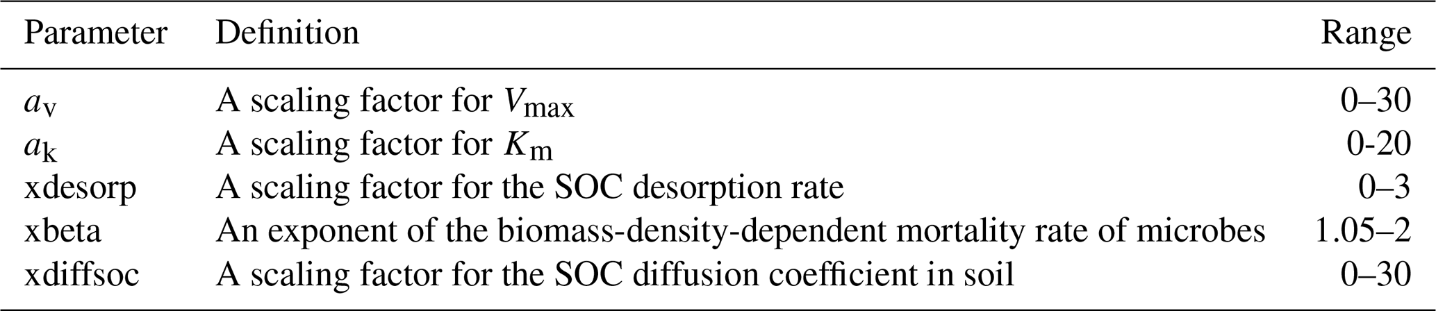
MIMICS parameters were derived from Zhang et al. (2020) and Wang et al. (2021), except that five parameters (Table 1) which directly control the organic carbon decomposition were optimised. An effective global optimisation algorithm called the shuffled complex evolution (SCE-UA, version 2.2) method (Duan et al., 1993) was applied for parameter optimisation by minimising the residual sum of squares between the observed and modelled values.

Vertically resolved MIMICS simulated the SOC concentration for 15 soil layers with a uniform layer thickness of 10 cm. As observations only provide one measurement for the top 30 cm of soil, we computed the average of the modelled values spanning the 0–10, 10–20 and 20–30 cm soil layers. This average was then adopted as the modelled SOC concentration for top 30 cm of soil, serving as the basis for evaluating the difference between observations and simulations.

Table 1 The optimised model parameters (dimensionless) and their value range.

Parameters in MIMICS were optimised for different groups divided based on two approaches. The first approach involved categorising all observations into four groups based on the plant functional type (PFT). The second approach used the most influential abiotic variables as predictors (as outlined in Sect. 2.2) and divided all observations into six clusters using the k-means algorithm. The determination of the optimal number of clusters was achieved through the minimisation of the sum of the within-cluster sum of squares of all clusters (WCSSE), a process facilitated by the “ClusterR” package in R (version 4.2.0). This clustering aimed to ensure the highest possible similarity among the environmental factors within each cluster. It was anticipated that the SOC ranges within each cluster would be narrow due to the high similarity of the environmental predictors.

2.4 Data

2.4.1 Predictors of spatial variations in the observed SOC concentration

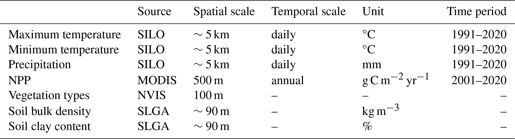
MIMICS requires the gridded mean annual temperature (MAT), carbon input and clay content as driving variables for a spatial simulation. The gridded mean annual precipitation (MAP) and vegetation types were also used during calibration and to aid in understanding the drivers and spatial variability in SOC. Details on the gridded data can be found in Table 2.

Gridded daily maximum temperature, minimum temperature and precipitation at 0.05° resolution were obtained from the SILO database (Jeffrey et al., 2001) of Australian climate data. Mean daily temperature was approximated as the average of the maximum and minimum daily temperature. MAT was calculated from the mean daily temperature from 1991 to 2020, and MAP was calculated from the daily precipitation from 1991 to 2020.

Carbon input was represented by the net primary production (NPP). The gridded mean annual NPP at 500 m was calculated based on the annual NPP from 2001 to 2020 obtained from MODIS (MOD17A3HGF V6.1) (Running and Zhao, 2021). NPP was partitioned into the aboveground and belowground parts by multiplying by the root-to-shoot ratio for different vegetation types (Mokany et al., 2006). Here, we did not account for the faction of NPP that is appropriated by human activities.

The distribution of vegetation types was obtained from the National Vegetation Information System (NVIS, version 6.0, https://www.dcceew.gov.au/environment/land/native-vegetation/national-vegetation-information-system, last access: 1 April 2024). Pixels of non-vegetated regions were removed, and 28 vegetation types from NVIS were aggregated to just 4 PFTs: forest, woodland, shrubland and grassland.

Soil bulk density and clay content were obtained from the maps of Soil and Landscape Grid National Soil Attributes (SLGA, Release 2; Grundy et al., 2015; Viscarra Rossel et al., 2015). Soil properties were predicted based on machine learning at depths of 0–5, 5–15, 15–30, 30–60, 60–100 and 100–200 cm in SLGA. Bulk density and clay content were estimated for the top 30 cm of soil as a weighted average of first three layers in the SLGA.

The initial spatial resolution of the gridded data was maintained when extracting the required environmental factors for each SOC observation. All data were then resampled to a 0.05° resolution using bilinear interpolation for the estimation of terrestrial SOC stocks at a continental scale.

Table 2 Information on the gridded data used in this study.

2.4.2 Soil organic carbon observations

SOC observations for the top 30 cm of soil in Australia were collected from two datasets. The first dataset is described in Viscarra Rossel et al. (2014) and Viscarra Rossel et al. (2019). We removed the observations collected from croplands based on the land-use record in the dataset as well as observations from unvegetated regions based on the NVIS vegetation map (see above). A total of 1070 site observations, including only 38 from forest soils, were retained. SOC stocks were reported in tonnes per hectare (t ha⁻¹). To better represent the SOC distribution in forests, we obtained additional forest SOC observations from a second dataset, the Biomes of Australian Soil Environments (BASE) described in Bissett et al. (2016). Here, SOC (%) was reported for 0–10 and 20–30 cm. We estimated SOC for the 0–30 cm soil depth following the method described in Viscarra Rossel et al. (2014).

To compare the observations with MIMICS outputs, we then converted both simulated SOC (mg cm⁻³) and observed SOC (t ha⁻¹) in the first dataset (Viscarra Rossel et al., 2014) to the SOC concentration (g C kg soil⁻¹) using the spatially explicit soil bulk density (BD) from the SLGA. The unit conversion will not affect the results of MIMICS. Soil clay content is extracted from the SLGA.

The spatial distribution of SOC observations from different PFTs is shown in Fig. 2a. The SOC concentration in the top 30 cm is positively skewed, ranging from 1.36 to 59.73 g C kg soil⁻¹ with a mean value of 9.97 g C kg soil⁻¹ and a median value of 6.11 g C kg soil⁻¹. The SOC concentrations in grassland, shrubland and woodland show similar distribution patterns (Fig. 2b), whereas the SOC concentration in forests is more variable, with a standard deviation of 15.92 g C kg soil⁻¹.

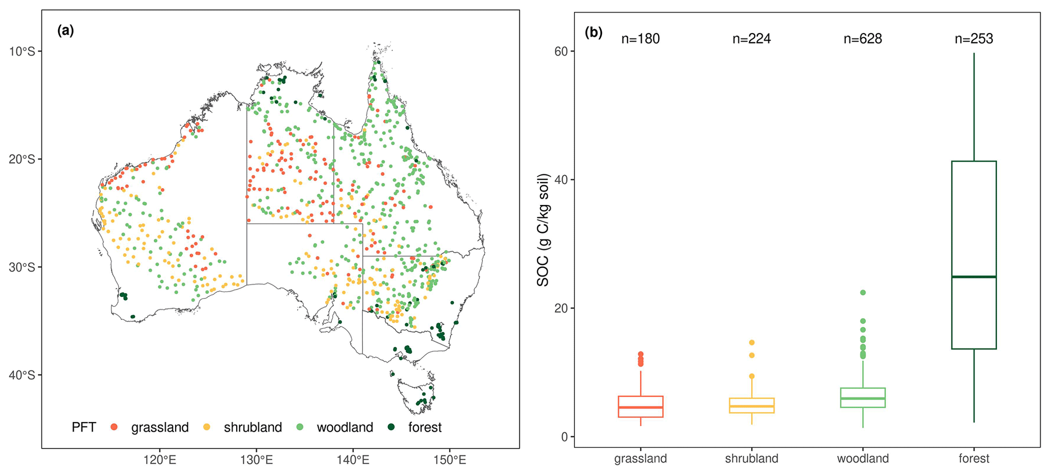
Figure 2 (a) Spatial distribution of the 1285 SOC observations used in this study and the PFTs that they belong to; (b) box plots of the SOC concentration distributions for each PFT. For box plots, centre lines represent the median value, upper and lower box boundaries represent the respective third and first quartiles, and the whiskers extend to the smallest and largest values within 1.5 times the interquartile range.

2.5 Model evaluation

For machine learning models, 70 % of the observations were randomly selected as training data to train the models, while the remaining 30 % of observations were used as test data to validate the predictions of the SOC concentration. For vertically resolved MIMICS, parameters were optimised for each PFT or environmental group (see Sect. 2.3 above); again, we randomly selected 70 % of observations in each group to train the model, while the remaining 30 % of observations were used for validation. To cross-validate, the procedure was repeated 10 times.

The performance of models was evaluated using four metrics: the mean absolute error (MAE) indicates how close the average predictions are to average observations; the root-mean-square error (RMSE) measures the overall accuracy, combining the mean, standard deviation differences (across sites) and (spatial) correlation; the coefficient of determination (R²) measures the percentage of variation explained by the model; and Lin's concordance correlation coefficient (LCCC; Lawrence and Lin, 1989) measures the level of agreement between predictions and observations following the 1:1 line. A good model will have an MAE and RMSE close to 0 and an R² and LCCC close to 1.

2.6 Estimation of terrestrial SOC stocks

SOC concentrations were used to train the models, and we then estimated terrestrial SOC stocks and their continental-scale spatial distribution in the top 30 cm of soil utilising the four models validated within this study. The SOC stock (t ha⁻¹) is calculated using the SOC concentration (g C kg soil⁻¹), bulk density (BD, kg m⁻³) and soil depth (m):

$$\begin{array}{}\text{(1)}& {\mathrm{SOC}}_{\mathrm{stock}}={\mathrm{SOC}}_{\mathrm{concentration}}\times \mathrm{BD}\times \mathrm{depth}/\mathrm{100}.\end{array}$$

In the cases of MIMICS-PFT and MIMICS-ENV, the initial step involved grouping all pixels into four distinct plant functional groups or six environmental clusters. As cross-validation was performed, the machine learning and process-based models were evaluated using test data, and the models with optimal performance were subsequently employed at each pixel to estimate the terrestrial SOC stocks. The map of the ensemble estimate of SOC stocks was produced as the average of the four model estimates at each pixel.

3 Results

3.1 Relative importance of predictors on SOC variation

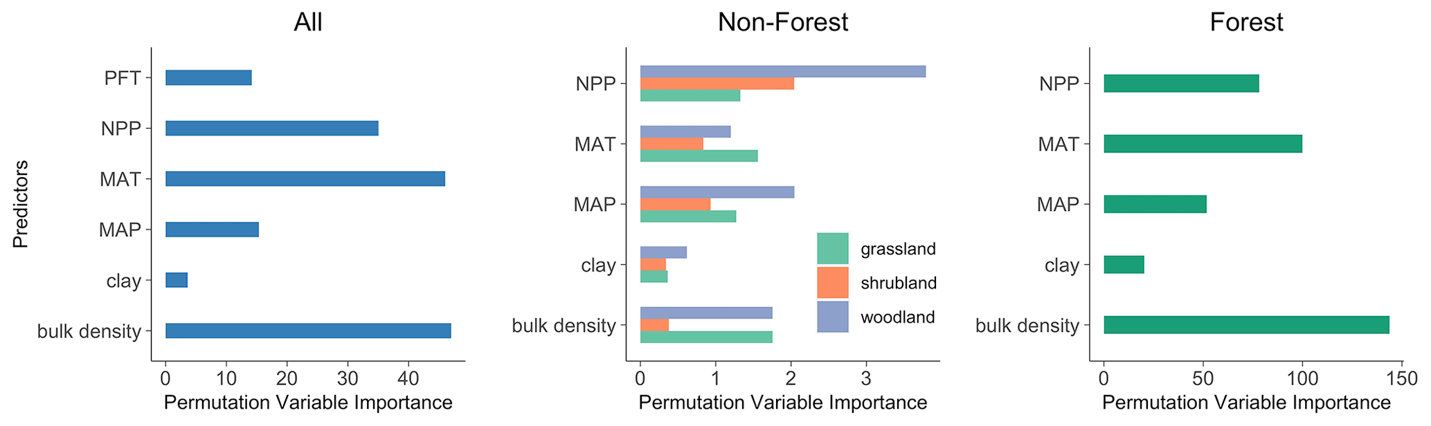
Using the PVI in random forest, we identified the significance of environmental factors with respect to predicting the SOC concentration. At the continental scale, the soil bulk density contributes most to the prediction of the SOC concentration, followed by the MAT, NPP and MAP (Fig. 3). The soil clay content and PFT exhibit relatively less significance in this regard.

The relative predictor importance for forests and grasslands aligns with the importance at the continental scale. In shrubland and woodland, the NPP and MAP emerge as the pivotal factors. Collectively, across both continental and regional scales, the soil bulk density, MAT and MAP are the three most influential abiotic factors.

Figure 3 Importance of predictors with respect to the SOC concentration for different PFTs.

3.2 Data clustering based on environmental factors

To develop the calibration groups for MIMICS-ENV, we partitioned the top three most important abiotic factors, which are soil bulk density, MAT and MAP, into six distinct clusters using k-means (see Sect. 2.3). The resulting characteristics and the spatial distribution of SOC belonging to these six clusters are illustrated in Fig. 4.

Notably, a substantial majority of forests were assigned to clusters 2 and 6 (Fig. 4a), while woodland, shrubland and grassland observations were distributed across the remaining four clusters. Among these clusters, cluster 5 exhibits the lowest SOC concentration, while the SOC of clusters 1 and 3 displays a comparable pattern but spread across different biomes. Conversely, the distribution of the SOC concentration in clusters 2, 4 and 6 shows more pronounced variability (Fig. 4c).

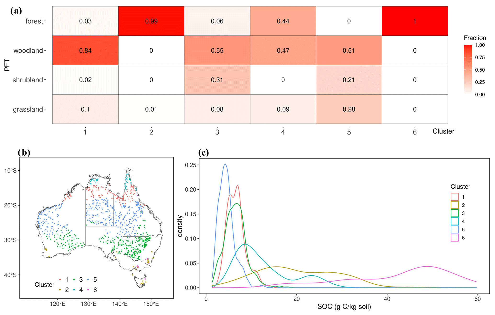
Figure 4 (a) The fraction of different PFTs in each cluster divided based on environmental factors; (b) the spatial distribution of the SOC observations from different environmental clusters; (c) a density plot of the observed SOC concentration for different clusters.

3.3 Evaluation of model performance

All models employed in this study (RF, k-means and MLR, MIMICS-PFT, and MIMICS-ENV) predicted the SOC concentration well for both the training data and the test data (Fig. 5). As anticipated, performance for both process-based models and machine learning models degrade using out-of-sample data vs. in-sample training or calibration data. When using test data, the mean R² value for all models ranges from 0.82 to 0.94, the mean LCCC ranges from 0.90 to 0.97, the mean RMSE ranges from 2.88 to 4.51 g C kg soil⁻¹ and the mean MAE ranges from 1.55 to 2.57 g C kg soil⁻¹.

The machine learning models outperformed MIMICS with respect to predicting the SOC concentration, regardless of the optimisation approach taken. Particularly, the RF model demonstrated the most accurate predictions, characterised by higher R² and LCCC values and lower RMSE and MAE values for both the training and test data. While MIMICS-ENV displayed performance similar to that of MIMICS-PFT with respect to the SOC concentration predictions based on the RMSE and MAE, the former exhibited slightly superior median R² and LCCC values, although with a higher variability (Fig. 5).

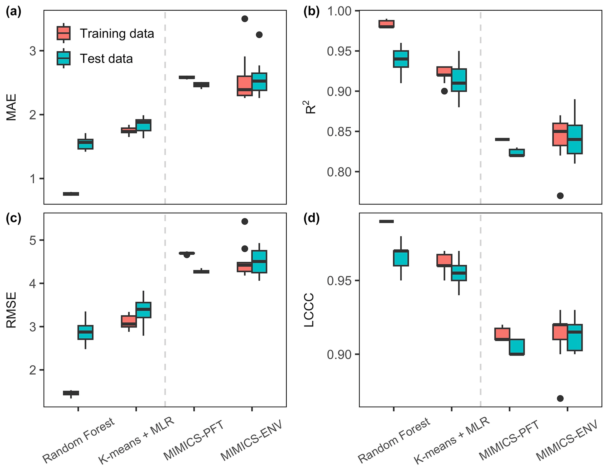
Figure 5 Performance metrics of the SOC concentration predictions. The units for MAE and RMSE are grams of carbon per kilogram of soil (g C kg soil⁻¹). The centre line represents the median value, the upper and lower box boundaries represent the respective third and first quartiles of metrics from cross-validation, and the whiskers extend to the smallest and largest values within 1.5 times the interquartile range.

The SOC concentration in forest soil exhibited significantly higher predictability than that in non-forest (woodland, shrubland and grassland) soil, as evidenced by a higher R² (ranging from 0.58 to 0.91) and LCCC (ranging from 0.75 to 0.95) for test data (Fig. 6). Machine learning models surpassed MIMICS with respect to predicting the SOC concentration for both forest and non-forest soils. Notably, MIMICS-ENV outperformed MIMICS-PFT with respect to SOC concentration predictions, particularly in non-forest soils.

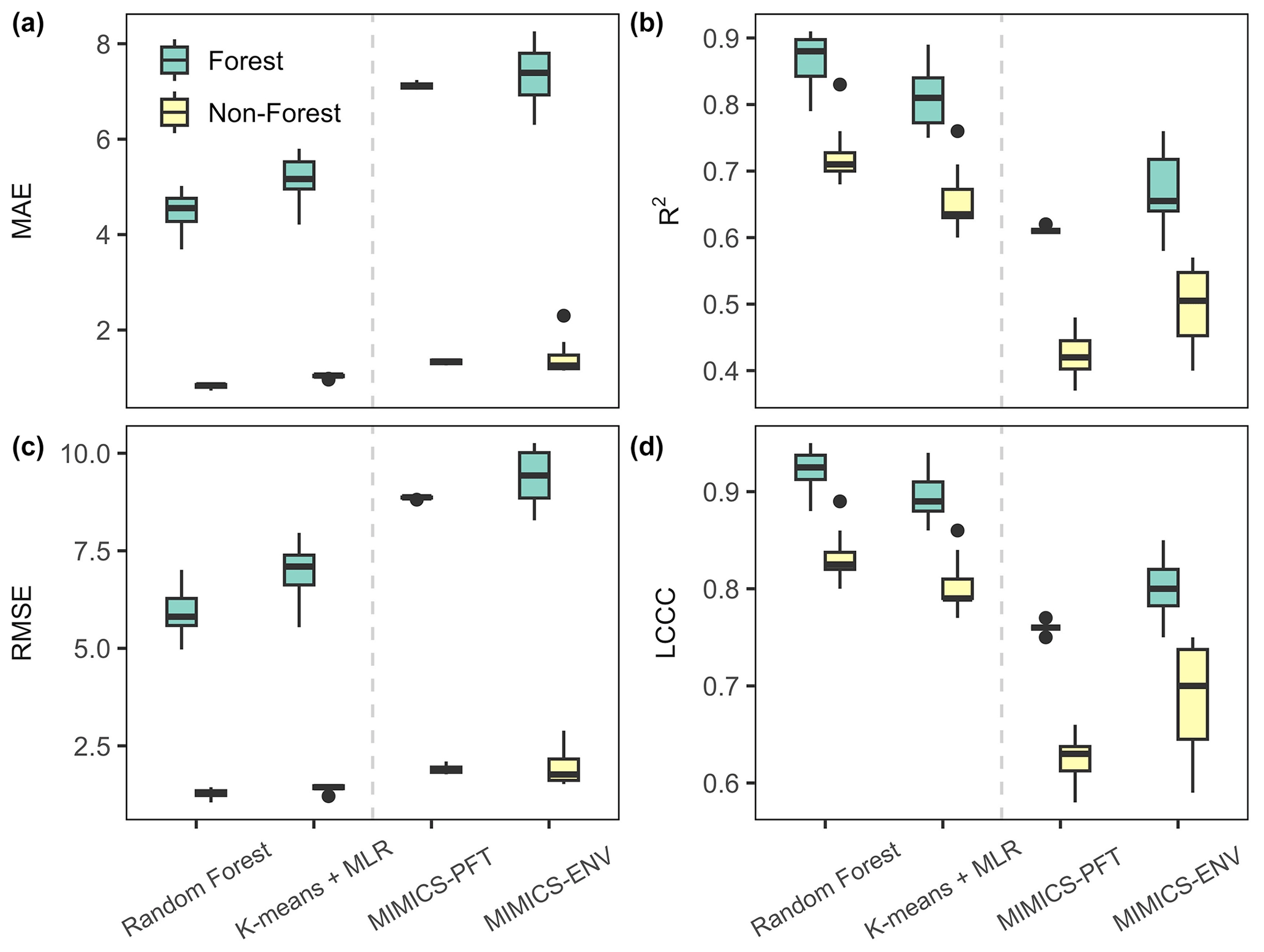
Figure 6 Performance metrics of the SOC concentration predictions for forest and non-forest (woodland, shrubland and grassland) soils in test (out-of-sample) data. The units for MAE and RMSE are grams of carbon per kilogram of soil (g C kg soil⁻¹). The centre line represents the median value, the upper and lower box boundaries represent the respective third and first quartiles of metrics from cross-validation, and the whiskers extend to the smallest and largest values within 1.5 times the interquartile range.

3.4 Estimations of terrestrial SOC stocks

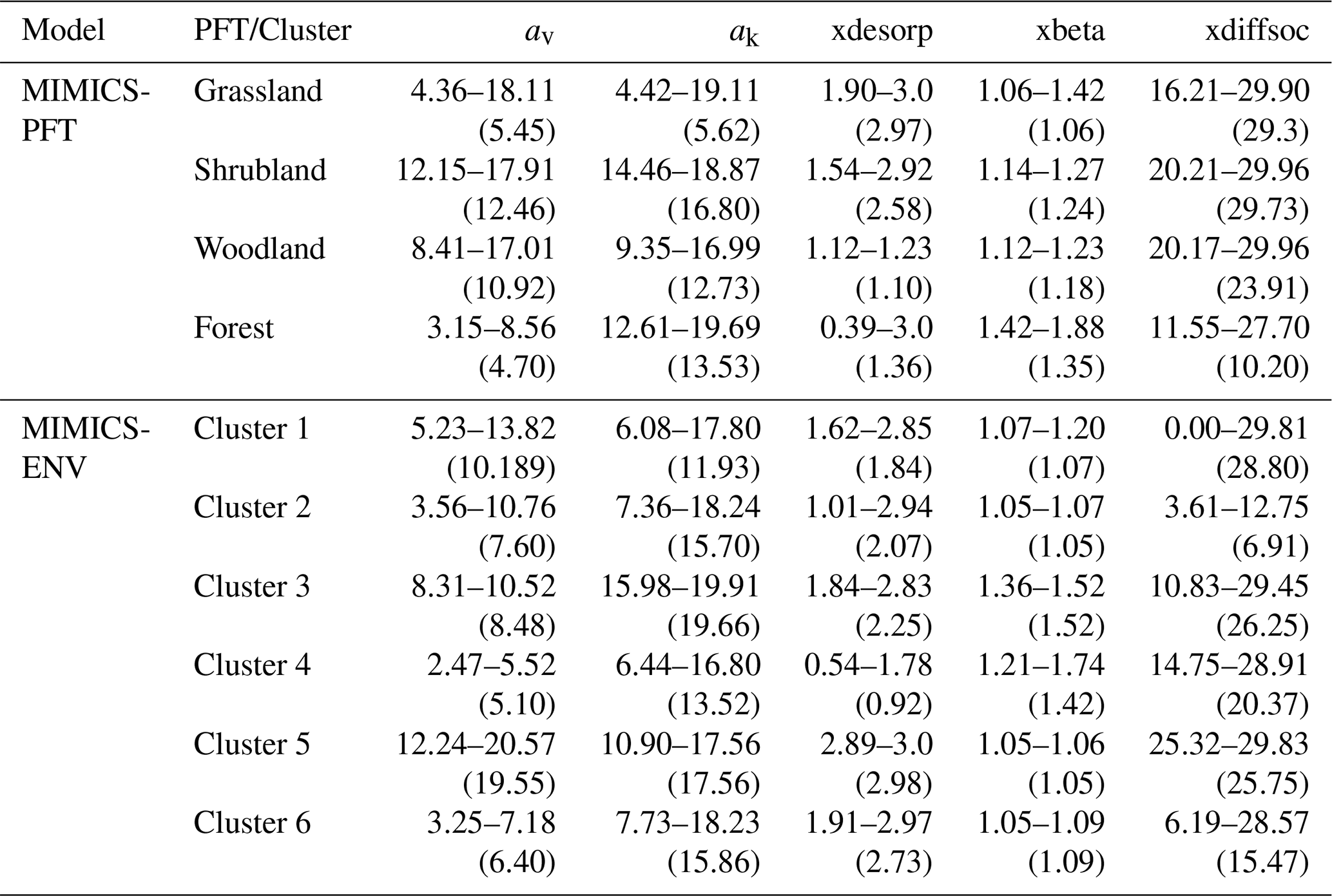
Using the best-fitted models after cross-validation (see Sect. 2.6 for details), we estimated the total SOC stock in the top 30 cm of soil for the whole Australian continent at a spatial resolution of 0.05° × 0.05°. The optimised parameters used for MIMICS-PFT and MIMICS-ENV at the continental scale are shown in Table 3.

Table 3 Optimised parameter ranges of MIMICS for cross-validation. Values in parentheses were used for estimating SOC stocks at the continental scale. The reader is referred to Table 1 for further explanations of each parameter.

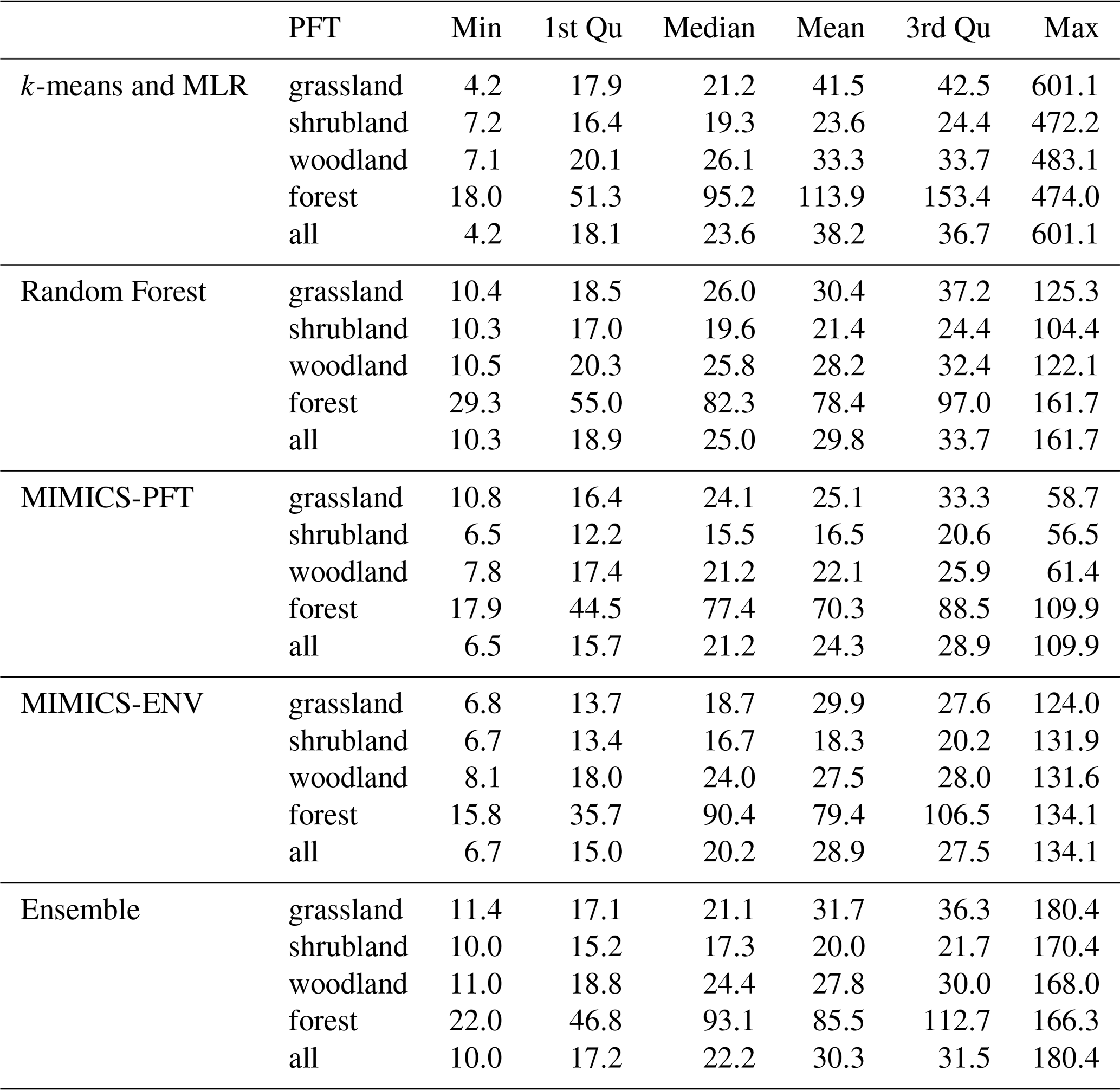
Descriptive statistics of predicted terrestrial SOC stocks at 0–30 cm soil depth are shown in Table 4. Forests have the largest mean SOC stocks, ranging from 70.3 to 113.9 t ha⁻¹, according to all models, whereas shrubland is estimated to have the lowest mean SOC stocks. The distributions of predicted continental SOC stocks by all models are positively skewed, with most estimated SOC stocks being less than 50 t ha⁻¹ (Fig. 7a); moreover, SOC stocks at peak density predicted by MIMICS-ENV and MIMICS-PFT are smaller than those predicted by the two machine learning approaches.

As expected, all models consistently projected larger SOC stocks in the south-eastern region, the south-western corner and Tasmania, whereas they consistently indicated lower SOC stocks in central and western Australia (Fig. 7b). Among the models, k-means coupled with multiple linear regression consistently provided the highest SOC estimations across all vegetation types, whereas the MIMICS-PFT model consistently yielded the lowest mean SOC stocks.

The ensemble estimate of SOC stocks (Fig. 7c) shows a similar distribution pattern to that generated by a single model. The SOC stocks of the ensemble range from 10.0 to 180.4 t ha⁻¹ with an average value of 30.3 t ha⁻¹. The coefficient of variation, calculated as the ratio of the standard deviation to the mean, across the four estimates (Fig. 7d) is positively correlated with the ensemble mean estimate. Thus, soils with higher SOC stocks exhibit greater variability in the SOC predictions among different models. Note also that the variability in estimates tends to be smaller in areas with denser numbers of observations (Fig. 7d).

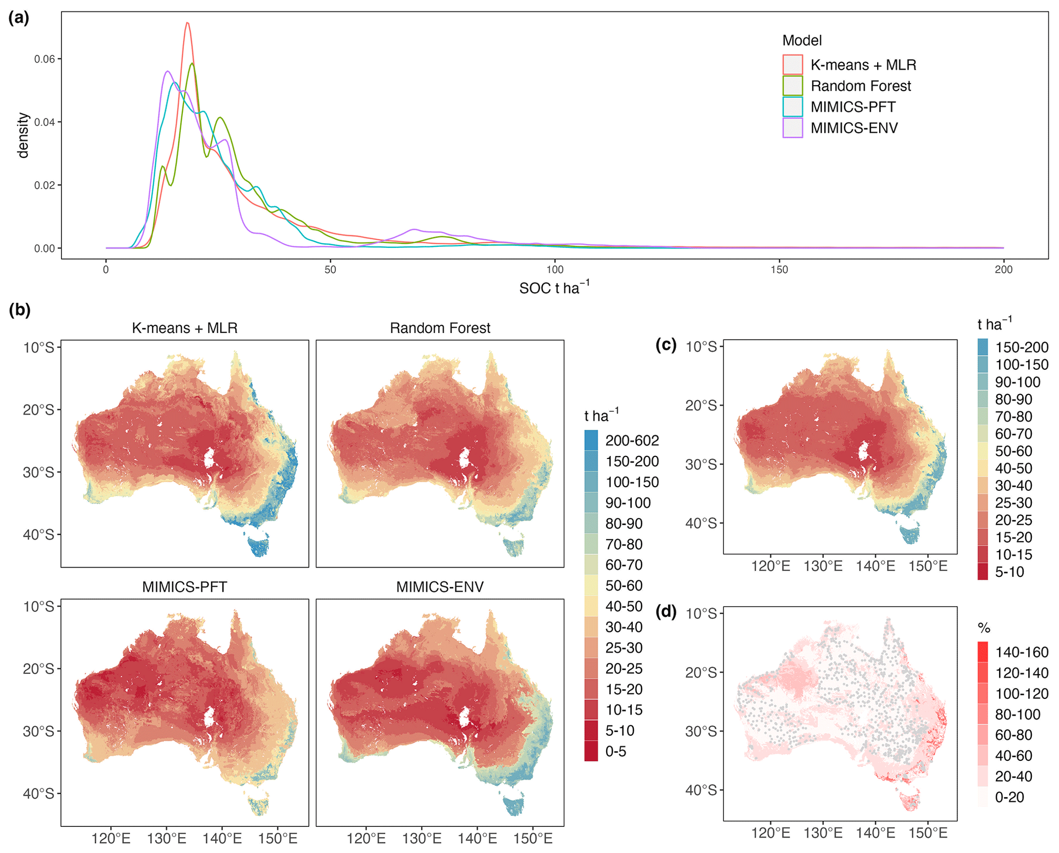
Figure 7 Estimated Australian terrestrial SOC stocks (t ha⁻¹) for the top 30 cm of soil and the ensemble statistical characteristics: (a) density plot of estimated terrestrial SOC stocks by all models, noting that only stocks less than 200 t ha⁻¹ are shown for better comparison of the distribution; (b) estimated SOC stocks by each model; (c) estimated SOC stocks of the ensemble; (d) coefficient of variation in the ensemble estimates of SOC stocks. Grey points represent the locations of SOC observations.

Table 4 Descriptive statistics of estimated terrestrial SOC stocks (t ha⁻¹) at 0–30 cm soil depth. Min and Max are the respective minimum and maximum values, while 1st Qu and 3rd Qu represent the respective first and third quartiles.

4 Discussion

4.1 Relative importance of predictors with respect to SOC variation

Extensive research has been conducted to discern the factors that govern SOC concentrations or stocks. Among the commonly employed predictors for SOC spatial variations, climate, organisms, topography, parent material and soil properties are prominent (Wiesmeier et al., 2019). Within this study, we conducted a comparative assessment of the significance of key variables, namely, MAT, MAP, NPP, soil clay content and bulk density, in driving variations in SOC in Australia. Although the number of predictors utilised in our approach is fewer than that employed in most digital mapping methodologies, our models show good performance with respect to predicting SOC in Australia (Figs. 5 and 6), and the strength of our technique lies in the potential for a more direct comparison between empirical and process-based models.

Consistent with the results of Hobley et al. (2015) on soils from eastern Australia, this study identified soil bulk density as an important predictor of the SOC concentration at the continental scale (Fig. 3). However, the relationship between soil bulk density and soil carbon concentration is largely interactive (Murphy, 2015). Higher concentrations of soil organic matter facilitate soil aggregation formation and increase soil porosity, which results in lower bulk density. Meanwhile, a soil with a reduced bulk density exhibits higher permeability for water and oxygen, which enhances plant root growth and SOC dynamics. Physically, the bulk density of organic matter is less than 1 g cm⁻³, much lower than soil mineral solids with a density of 2.66 g cm⁻³. Therefore, soils of lower bulk density usually have a higher SOC concentration (Marshall et al., 1996).

Across the Australian continent, MAT emerges as the second most influential factor governing SOC variations, followed by NPP, MAP and clay content. This sequence of significance diverges from the findings of Walden et al. (2023), who observed the following order of importance at the continental scale in Australia: NPP > clay content > MAP > MAT. The number of predictors used in their study was much higher than that in our study, which may have affected the contribution of given predictors to the SOC variation (Guo et al., 2019). However, this discrepancy might also be attributable to the utilisation of observations encompassing both terrestrial and blue-carbon ecosystems in their study. Clay mainly emerges as key driver in groups in which aquatic plants (e.g. seagrass and tidal marsh) appear. The more extensive dataset encompassing the eastern coastline, characterised by greater variability and abundance of NPP input, potentially elevates the NPP to a dominant role in influencing SOC variations within their study.

For SOC in different vegetation types (Fig. 3), soil bulk density and MAT are more important than other factors in forests, and all factors except clay content showed similar importance with respect to predicting the SOC concentration in grasslands. The NPP and MAP dominate the SOC variations in woodlands and shrublands. Climate conditions, as represented by MAT and MAP, exert their impact on SOC in all vegetation types. It was proposed that the primary climatic determinant of SOC variation hinges on the primary constraint affecting SOC production and turnover (Hobley et al., 2016). In this study, most shrublands and woodlands are distributed in arid and semi-arid regions characterised by limited precipitation, which leads to water stress in the surface soil, limiting plant productivity and reducing soil C input (Hobley et al., 2015). Consequently, MAP and NPP exhibited a relatively higher influence on SOC variations in soils under these vegetation types. In contrast, forest SOC observations are mainly distributed in areas with relatively lower temperatures; therefore, these regions experience constrained microbial metabolism, leading to reduced decomposition rates and high SOC accumulation (Wynn et al., 2006). Thus, MAT emerges as a key factor influencing SOC variations in forests. Furthermore, it is noteworthy that the soil bulk density plays a crucial role in determining the SOC distribution within forests, where it is found to be significantly lower compared with other vegetation types. This lower soil bulk density likely improves oxygen availability to soil microbial communities and facilitates the formation of microaggregates to enhance the preservation of SOC within the soil matrix (Bronick and Lal, 2005). Consequently, it effectively contributes to elevated SOC concentration levels in forested areas.

PFT is the only categorical predictor of the SOC concentration in this study. SOC is mainly derived from plant C input through aboveground and belowground tissues, and SOC turnover and storage are influenced by plant traits, such as plant growth rate and chemical and physical composition (De Deyn et al., 2008; Faucon et al., 2017). With the shared representation of similar plant traits, the PFT is widely used in process-based models (Poulter et al., 2015; Famiglietti et al., 2023). It was found that the vertical distribution of SOC is highly related to the PFT due to differences in root distribution and aboveground and belowground allocation (Jobbágy and Jackson, 2000). However, our study is limited by the absence of SOC observations at multiple soil depths, restricting the analysis to the spatial distribution of SOC at 30 cm soil depth. The influence of the PFT on the SOC concentration at this particular depth appears to be relatively insignificant (Fig. 3), casting doubt on the effectiveness of optimising parameters of process-based models for individual PFTs (Cranko Page et al., 2024). Considering this, employing the top three influential abiotic predictors, soil bulk density, MAT and MAP, we partitioned all observations into six distinct clusters using k-means. It was anticipated that the SOC ranges within each cluster would be narrow due to the high similarity of these three predictors within each group. However, the distribution of SOC in clusters 2, 4 and 6 exhibited considerable variability (Fig. 4). Given that these clusters are predominantly composed of forests, it becomes apparent that these three abiotic factors alone are insufficient to fully characterise the intricacies of the forest SOC concentration. It was found that elevation and evapotranspiration also drive the variation in the forest SOC in Australia (Walden et al., 2023); thus, taking these factors into account might potentially increase the predictability of forest SOC.

4.2 Model evaluation and comparison with other studies

Although the predictors used for machine learning models are not exactly same as the inputs of MIMICS, the missing factors (e.g. MAP) were used for parameter optimisation of MIMICS-ENV, making the predictions dependent on similar information and, therefore, comparable to some extent. Moreover, our study presented clear evaluation metrics for out-of-sample validation, enabling a more robust assessment of model performance when applied to new datasets.

Based on the performance metrics of test data, the machine learning models performed remarkably well (Fig. 5). The R² values suggested that both machine learning models can explain more than 90 % of SOC variability across sites, and random forest did the best job, with the greatest R² and LCCC values and the lowest MAE and RMSE values. Random forest algorithms have been widely adopted for predicting spatial–temporal SOC dynamics and have produced moderately good performance both regionally and globally. For example, Wang et al. (2022) applied random forest to estimate SOC stocks in south-eastern Australia and explained 69 % of the variation in the current SOC stocks. Nyaupane et al. (2023) trained a random forest model using global SOC observations and explained 61 % of SOC variation. The good performance of random forest might be attributed to a reduced susceptibility to overfitting and a better capacity to manage the hierarchical non-linear relationships that exist between SOC and environmental predictors (Wang et al., 2018b). Other machine learning methods have been applied to predict continental SOC stocks in Australia. For example, Walden et al. (2023) trained the CUBIST regression tree algorithm to predict SOC stocks for the top 30 cm of soil using the Harmonized datasets. The mean LCCC and RMSE values for out-of-sample validation in their study were 0.78 and 0.20, respectively, when log₁₀-transformed SOC (t ha⁻¹) values were used. Wadoux et al. (2023) applied quantile regression forest to predict SOC stocks at multiple soil depths. The prediction accuracy decreased dramatically for deeper depth intervals, with the greatest R² value (0.53) being found at 0–5 cm soil depth. The better results in this study may be attributed to the removal of cropland ecosystems, which are clearly highly managed and, therefore, less predictable. Agricultural practices greatly affect SOC stocks in Australia and add the complexity to the relationship between SOC and environmental factors (Luo et al., 2010). Models using environmental predictors without representation of land-use management are unlikely to be able to fully capture the SOC dynamics in croplands (Abramoff et al., 2022).

Although MIMICS was not as accurate as machine learning models with respect to simulating spatial variation in the SOC concentration in Australia, it did well at the continental scale with a mean R² value of 0.82 and 0.84 for MIMICS-PFT and MIMICS-ENV, respectively (Fig. 5); these R² values are much greater than the values (<0.4) obtained by Abramoff et al. (2022), who applied a different microbial explicit model to the Australian SOC dataset. Georgiou et al. (2021) found that there was a mismatch between observations and MIMICS regarding the role of different environmental controls on SOC variability at the global scale. In their study, NPP and MAT had the most explanatory power for SOC stocks from MIMICS, while clay content had the most explanatory power for global SOC observations, which limits the predictability of SOC using MIMICS in their study. However, in our study, NPP and MAT (rather than clay content) played a greater role in observed SOC variations, perhaps contributing to better predictive performance for MIMICS in Australia. It also means that SOC estimates in our study are highly sensitive to the estimates of NPP. In this study, we used the MODIS NPP product (Running and Zhao, 2021) and did not account for the loss of NPP due to human activities, which may likely influence the optimised estimates of some model parameters, and the uncertainties in the simulated SOC concentration. Future studies would ideally use multiple NPP products to quantify the impacts of NPP uncertainties on simulating SOC variation in Australia.

The modest performance of the MIMICS process-based model relative to machine learning models could potentially be attributed to the absence of the explicit representation of MAP. The augmentation of MAP within parameter optimisation in MIMICS-ENV did allow for improved performance compared with MIMICS-PFT, particularly within non-forest regions where the importance of MAP rivals or surpasses that of temperature. Precipitation is a determinant of plant productivity, especially in arid and semi-arid regions. Furthermore, arid regions with limited precipitation are characterised by a lower weathering rate, limiting the formation of mineral-associated soil carbon (Doetterl et al., 2015). Hence, we assume that introducing the effect of moisture to MIMICS could contribute to a more accurate prediction of SOC, compared with just taking MAP into account for parameterisation, especially in arid and semi-arid regions.

All models produced lower MAE and RMSE values for non-forest SOC but higher R² and LCCC values for forest SOC (Fig. 6). SOC in forests is more abundant and variable compared with SOC in other vegetation types, even when climate conditions are similar, which leads to greater absolute error in the estimated forest SOC than in other vegetation types. However, in terms of the consistency and concordance between the pattern of observations and predictions, all models show a higher ability to predict SOC in forests. Forests, given that they are less-perturbed ecosystems, might show greater SOC predictability due to the reduced influence of direct anthropogenic disturbances. Grasslands, shrublands and woodlands, predominantly situated in Australian rangelands, may experience extensive grazing and land management. Primarily, grazing reduces soil carbon input via the consumption of aboveground biomass and accelerates SOC decomposition through the input of nutrient-enriched animal waste. This introduces additional uncertainties to our modelled SOC estimates, as C input is solely represented by NPP without accounting for the impact of grazing and land management. Moreover, the cascading effects of grazing extend to potential alterations to plant composition and structural attributes, inducing consequential shifts in litter properties that modulate soil carbon decomposition kinetics (Lunt et al., 2007; Bai and Cotrufo, 2022). The disturbances triggered by grazing manifest in soil carbon pools, leading to a state of disequilibrium rather than adhering to the assumption of SOC convergence toward equilibrium, as embraced in this study's framework. Notably, forests, as relatively undisturbed natural ecosystems, demonstrate a better coherence with the equilibrium assumption, rendering their SOC more amenable to prediction through environmental drivers.

4.3 Spatial prediction of SOC stocks in Australia

We produced gridded SOC stocks across Australia using the models validated in this study and an ensemble estimate as the average of four models (Fig. 7). Among the models, k-means coupled with multiple linear regression produced the largest mean SOC stocks at both the continental scale and for all vegetation types. In contrast, RF and MIMICS, with different parameterisation approaches, produced lower SOC stock estimations (Table 4). The mean terrestrial SOC stocks estimated by random forest and MIMICS are comparable with that estimated by the Australian baseline map, which was generated using a machine learning algorithm, reporting mean SOC stocks of 29.7 t ha⁻¹ with 95 % confidence limits of 22.6 and 37.9 t ha⁻¹ (Viscarra Rossel et al., 2014). However, SOC stocks might be underestimated by these methods because of the scarcity of data from the most productive temperate forest in both the baseline map (Bennett et al., 2020) and in our study. The parameter optimisation process of MIMICS and the training process of random forest are greatly affected by the data used to train the model. Most SOC observations in this study were sourced from arid and semi-arid regions that are characterised by a relatively low SOC content. As a result, the models' ability to predict SOC stocks beyond the observed data range is somewhat constrained. PFT was found to be less important than other environmental factors in driving spatial SOC variations (Fig. 3); thus, it was perhaps not surprising that applying parameters optimised for each PFT to the regions with the same PFT but broader climate conditions led to inferior results compared with applying parameters optimised for each environmental group.

The utilisation of linear regression in the k-means and MLR model generated SOC estimates beyond the range of observations, particularly in eastern Australia where environmental conditions deviate from the training data. The mean SOC stocks estimated by k-means and MLR (38.2 t ha⁻¹) are higher than those of the other models employed in this study, and they align closely with the mean value of 36.2 t ha⁻¹ reported by Walden et al. (2023), who updated the Australian baseline SOC map (Viscarra Rossel et al., 2014) by incorporating additional SOC observations from forests and coastal marine ecosystems. However, caution is required when interpreting extreme values derived from the k-means and MLR model, such as the instance of grassland SOC stocks reaching 601 t ha⁻¹ (Table 4). These values raise concerns about the reliability of this approach when undertaking out-of-sample extrapolation. Although there is a positive relationship between NPP and SOC observations in this study, SOC accumulation cannot continuously increase linearly in the regions where environmental conditions seem highly conducive to SOC formation. The greater amount of carbon input in eastern Australia might trigger the acceleration of microbial decomposition because of a priming effect, thereby leading to a decreased accumulation of SOC stocks (Ren et al., 2022). The existence of SOC saturation also implies that SOC cannot be accumulated without limit (Georgiou et al., 2022; Viscarra Rossel et al., 2023). In light of these complexities, applying linear regression to predict SOC stocks, especially under extreme environmental conditions, should be undertaken with care.

Continentally, higher SOC stocks were estimated for the south-western corner and south-eastern region of Australia (Fig. 7), aligning with other SOC maps for Australia (Wadoux et al., 2023; Walden et al., 2023). These regions are characterised by lower temperature and higher precipitation; therefore, high SOC accumulation appeared because of a high NPP carbon input and a low decomposition rate. However, the high variability in the SOC estimates among the four models in these regions should be highlighted (Fig. 7d), along with the difference in magnitudes between the estimates in this study and other Australian SOC products (Viscarra Rossel et al., 2014; Walden et al., 2023). Despite inherent differences in model structures, the scarcity of observations in these regions likely contributes to the large uncertainties in SOC estimates. Forests have the largest mean SOC stocks, ranging from 70.3 to 113.9 t ha⁻¹, estimated by the four models in this study. Around 75 % of the forest SOC is from soil under eucalypt open forest, and mean SOC stocks under this type of forest were estimated to be 87.5 t ha⁻¹ (95 % confidence interval of 63.8–119.6 t ha⁻¹) (Walden et al., 2023). Shrublands are estimated to have the lowest mean SOC stocks, and more than 90 % of shrub SOC observations are from soil under Acacia shrubland and chenopod shrubland, which rank at the bottom of SOC stocks among different vegetation types (Walden et al., 2023). The low SOC in shrubland is probably due to low carbon input because of limited rainfall (MAP <280 mm). Although the mean SOC stocks in non-forest regions are much smaller than values for forests, the greater area of vegetation cover results in considerable total SOC stocks, highlighting the importance of carbon building and maintenance via improved management in these areas. Greater variability in the SOC estimates among different models appears in the regions where SOC stocks are higher (Fig. 7). The sparsity of SOC observations is a primary contributor to the uncertainties associated with SOC estimates in these regions, highlighting the importance of continual data collection to better constrain models' behaviour. This imperative is especially pronounced in regions covered by forests, as forested soils exhibit substantial SOC stocks, amplifying the significance of abundant and accurate data acquisition in these specific ecosystems.

5 Conclusions

We compared the performance of two machine learning models and one process-based microbial model employing two parameterisation approaches in order to explain the spatial variation in the SOC concentration in the top 30 cm of soil in Australia. We found that climate conditions and NPP contribute more than soil clay content to predicting the SOC concentration in Australia.

Validation results affirm that, with appropriate filtering of data (e.g. removing highly managed crop ecosystems), models can predict the SOC concentration at the continental scale with reasonably high reliability, achieving explained variances exceeding 80 % for out-of-sample test data, with random forest showing the highest prediction accuracy. Notably, all models show higher R² values for the prediction of SOC in forests compared with non-forest soils. MIMICS, with parameters optimised for different environmental clusters, performed better with respect to SOC prediction than MIMICS with parameters optimised for different PFT, especially in non-forest regions.

All models broadly agree on the spatial distribution of SOC stocks, with higher SOC stocks concentrated in the south-eastern and south-western regions of Australia. However, the variations in estimated values need to be acknowledged, particularly in highly productive regions. Among these estimates, the k-means algorithm coupled with multiple linear regression yields the highest mean SOC stock estimate, whereas the MIMICS-PFT model generates the lowest estimate. Considerable disagreement regarding the maximum and minimum SOC stock values predicted by all models exists, partly because models are less constrained by observations in these environments, highlighting the need for continued observational campaigns.

Our investigation has revealed significant disparities in estimated SOC stocks when different methodologies are employed. This highlights the need for a critical re-evaluation of land management strategies that heavily depend on SOC estimates derived from a single approach. The incorporation of an ensemble of SOC estimates is more likely to effectively capture elements of the uncertainty associated with SOC estimations, providing a more robust basis for informing strategies regarding soil carbon management and climate change mitigation.