Addressing soil data needs and data gaps in catchment-scale environmental modelling: the European perspective

To effectively guide agricultural management planning strategies and policy, it is important to simulate water quantity and quality patterns and to quantify the impact of land use and climate change on soil functions, soil health, and hydrological and other underlying processes. Environmental models that depict alterations in surface and groundwater quality and quantity at the catchment scale require substantial input, particularly concerning movement and retention in the unsaturated zone. Over the past few decades, numerous soil information sources, containing structured data on diverse basic and advanced soil parameters, alongside innovative solutions to estimate missing soil data, have become increasingly available. This study aims to (i) catalogue open-source soil datasets and pedotransfer functions (PTFs) applicable in simulation studies across European catchments; (ii) evaluate the performance of selected PTFs; and (iii) present compiled R scripts proposing estimation solutions to address soil physical, hydraulic, and chemical data needs and gaps in catchment-scale environmental modelling in Europe. Our focus encompassed basic soil properties, bulk density, porosity, albedo, soil erodibility factor, field capacity, wilting point, available water capacity, saturated hydraulic conductivity, and phosphorus content. We aim to recommend widely supported data sources and pioneering prediction methods that maintain physical consistency and present them through streamlined workflows.

1 Introduction

The availability of raw and derived soil datasets, specifically regarding soil hydraulic data, has increased significantly in Europe over the last 10 years as a result of the European Green Deal, specifically through initiatives and strategies aimed at promoting sustainable land use, soil health, and environmental protection (Montanarella and Panagos, 2021). Both the collection and harmonization of soil datasets and the preparation of soil maps have intensified. Further to these improvements, the derivation of prediction algorithms, which can compute specific soil properties from easily available soil or other environmental variables (the pedotransfer functions (PTFs)), has continued to be refined since the 1980s. The growing amount of spatiotemporal environmental data opens up possibilities for different prediction approaches, which is reflected in the terminology of the transfer functions – e.g. (i) the classical PTFs mostly use only soil properties as input (Bouma, 1989); (ii) those PTFs that consider not only soil properties but also other environmental variables are called covariate-based geo-transfer functions (Gupta et al., 2021a); and (iii) spectral transfer functions predict soil properties that are not easily available from spectral data (Babaeian et al., 2015), while machine-learning-based (ML-based) soil mapping fuses prediction algorithms with geostatistical methods (Romano et al., 2023). All these improvements resulted in the emergent availability of soil maps at global, regional, and local scales.

In most cases, the basic soil properties, i.e. soil organic carbon content and particle size distribution, are locally available at a high resolution (< 100 m), but information on bulk density, albedo, soil erodibility factor, soil hydraulic properties, and soil nutrient content is often lacking. There are many PTFs available in the literature that can be used to calculate soil physical (Abbaspour et al., 2019) and hydrological (Bouma and van Lanen, 1987; Van Looy et al., 2017) parameters from basic soil properties, but determining the most suitable one might not be obvious. Parameter estimations derive the parameters of a model that describes either water retention, hydraulic conductivity, or both across the entire matric-potential range. These estimations aim to ensure a cohesive physical relationship between the computed soil hydraulic properties.

Information on soil nutrient properties that is often essential for environmental modelling, such as plant-available soil phosphorus or soil nitrate content, is seldom accessible at a catchment or regional scale. In the absence of measured data on nutrient content, estimating highly mobile nutrients like nitrate poses a challenge due to seasonal fluctuations influenced by factors such as fertilizer application, rainfall, harvest cycle, plant nutrient uptake, and microbial activity. Regarding plant-available phosphorus, its levels typically exhibit minimal variation throughout a year. Therefore, approximating its quantity could be reliant on land use type and area-specific phosphorus fertilization loads (Ballabio et al., 2019). Nevertheless, multiple methods are employed across Europe to measure plant-available soil phosphorus content, potentially requiring conversions between these methods for broader-scale applications. A comprehensive review on conversion equations is available specifically for European studies in Steinfurth et al. (2021).

Often, those soil properties are required as model input data as well, which are rarely available. One example is the data on soil cracking, which are rarely readily available. Cracking intensity and the number of cracks are determined by (i) soil mineralogy, specifically the number and type of clay minerals; (ii) the type of strength that forms the soil structure (Lal and Shukla, 2004); and (iii) human activity, e.g. tillage and plant spacing. The aperture and closure of cracks can be dynamically related to soil water content (Xing et al., 2023). The data that could describe the variability of cracking are also not easily available; therefore, prediction of this parameter is limited at the catchment scale.

Dai et al. (2019b) provide an extensive review on global soil property maps applicable for Earth system models. Abbaspour et al. (2019) collected both soil datasets and pedotransfer functions for global Soil and Water Assessment Tool (SWAT) applications. From these comprehensive global review studies and a variety of soil datasets available from, among others, the European Soil Data Centre (Panagos et al., 2022) (https://esdac.jrc.ec.europa.eu/, last access: 2 September 2024) or ISRIC – World Soil Information (https://www.isric.org/, last access: 2 September 2024), it is not straightforward which data and/or pedotransfer functions could be used for environmental modelling in European case studies. Therefore, in this study, we support soil data retrieval for environmental modelling across Europe by (i) systemizing the information on open-access datasets and PTFs applicable for Europe, (ii) demonstrating and quantifying the difference between some PTFs and prediction approaches to cover missing soil properties based on the point data of EU-HYDI, and (iii) providing a comprehensive workflow and accompanying open-source R script and library for the derivation of missing soil data. For the selection of the prediction approaches, three requirements had to be fulfilled: (1) the prediction algorithm had to be trained on temperate soils and should not be specific to a particular soil reference group, (2) the required predictors had to be available in most of the open-access soil datasets, and (3) it should have notable ease of application. Hence, despite certain published prediction methods specifying soil depth, texture, and organic matter as requirements, those reliant on, for instance, artificial neural networks, lacking a user-friendly interface, or integration into accessible tools like R packages or Python modules, were excluded from testing due to their challenging application. For ease of reference, all the equations needed to calculate the most-often-required soil input parameters are given below.

Table 1 Open-access soil data that could be applied for environmental modelling in the European Union.

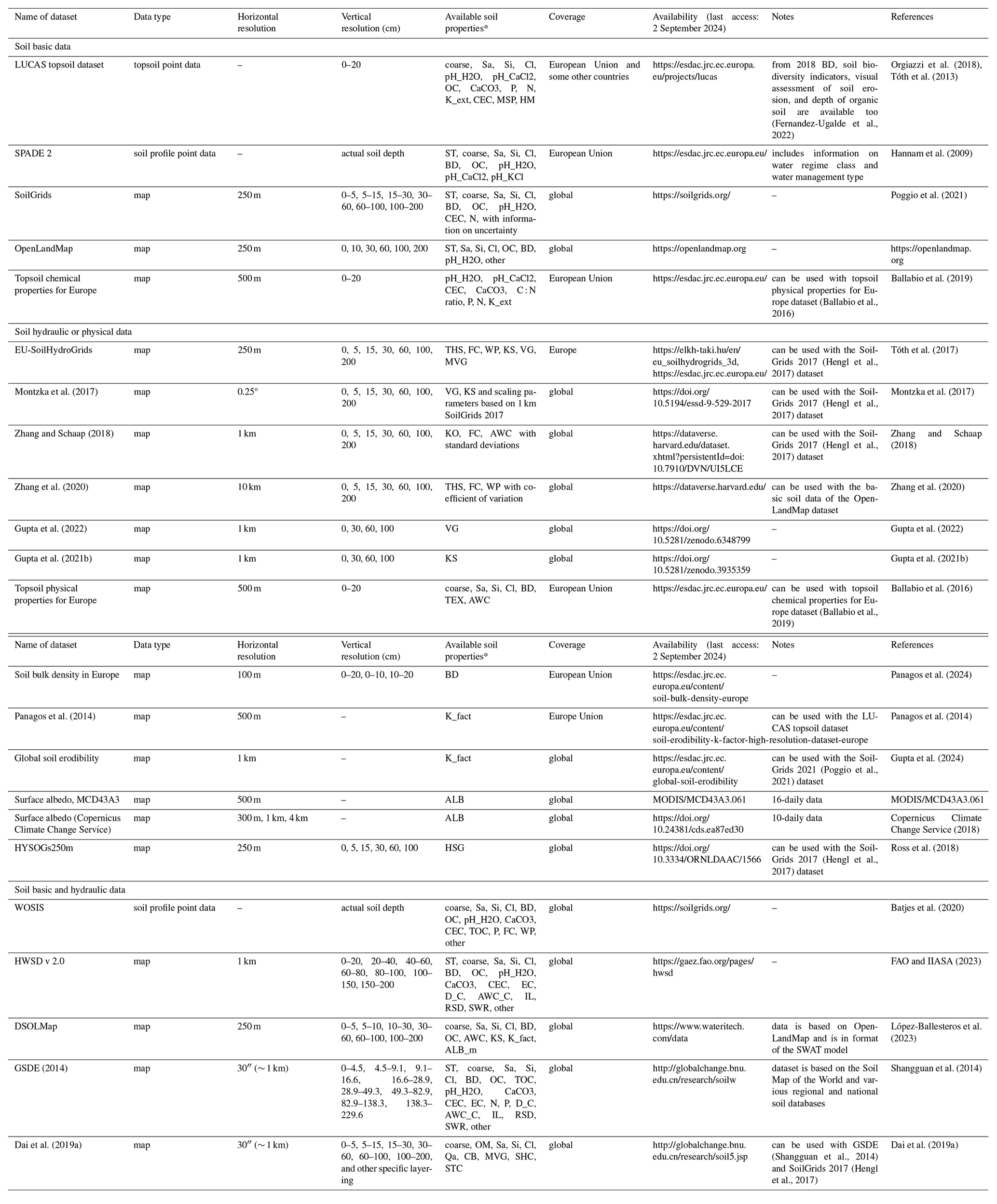
^* ST refers to soil type; coarse refers to coarse fragments; Sa, Si, and Cl refer to sand, silt, and clay content; Qa refers to quartz content of the mineral soil; BD refers to bulk density; OM refers to organic matter content; OC refers to organic carbon content; TOC refers to total organic carbon content; pH_H2O refers to pH in water; pH_CaCl2 refers to pH in calcium chloride; pH_KCl refers to pH in potassium chloride; CaCO3 refers to calcium carbonate content; CEC refers to cation exchange capacity; EC refers to electrical conductivity; N refers to total nitrogen content; K_ext refers to extractable potassium content; P refers to phosphorus content extracted by Olsen method; MSP refers to multispectral property; HM refers to heavy metal; K_fact refers to soil erodibility (K factor) based on the Revised Universal Soil Loss Equation; ALB refers to surface albedo; ALB_m refers to moist soil albedo; HSG refers to hydrological soil group based on the National Engineering Handbook of the US Department of Agriculture Natural Resources Conservation Service (2009); D_C refers to drainage class, AWC_C refers to available water capacity class in the rootable depth; IL refers to depth class to impermeable layer; RSD refers to rootable soil depth class; SWR refers to soil water regime class; THS refers to saturated water content; FC refers to water content at field capacity; WP refers to water content at wilting point; KS refers to saturated hydraulic conductivity; VG refers to parameters of the van Genuchten model used to describe the soil water retention curve (θ_s, θ_r, α, n, m); MVG refers to parameters of the Mualem–van Genuchten model used to describe the soil water retention and hydraulic conductivity curve (θ_s, θ_r, α, n, m, K₀, L); CB refers to parameters of the Campbell model used to describe the soil water retention and hydraulic conductivity curve (θ_s, ψ, λ, K_S); KO refers to parameters of the Kosugi model used to describe the soil water retention and hydraulic conductivity curve (θ_s, θ_r, h_m, σ, K_S); SHC refers to heat capacity of soil solids; STC refers to soil thermal conductivity of unfrozen saturated soil, frozen saturated soil, and dry soil; other refers to other soil properties, which are less frequently required by environmental models; AWC refers to available water capacity; and TEX refers to USDA soil texture class.

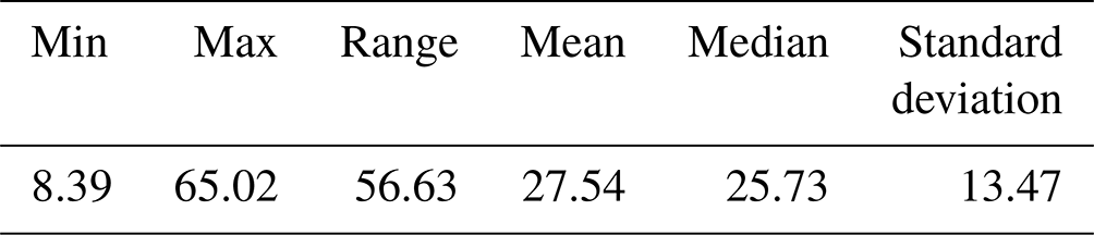
Table 2 Descriptive statistics of the locally measured phosphorus content, converted to Olsen P, from 34 agricultural parcels.

2 Materials and methods

We distinguish and list soil physical and chemical parameters similarly to the terminology used by the Soil and Water Assessment Tool model documentation (Neitsch et al., 2009). We include the prediction of soil porosity since this parameter is frequently used in environmental models, e.g. MIKE SHE (DHI, 2023), HEC RAS (US Army Crops of Engineers, 2024), and PIHM (Li and Duffy, 2011). It is noteworthy that some models and accompanying model setup tools have an internal built-in PTF to compute porosity, e.g. SWAT+. The codes to compute the soil parameters were built based on the structure and terminology used by the SWAT+ usersoil table (Arnold et al., 2012). Soil properties most frequently required by the environmental models (based on, e.g. Abbaspour et al., 2019; Dam et al., 2008; Dang et al., 2022; DHI, 2023; Hansen et al., 2012; Šimùnek et al., 2012; Yu et al., 2020) are

• soil layering

• maximum rooting depth;

• effective bulk density;

• field capacity;

• wilting point;

• available water capacity;

• porosity;

• saturated hydraulic conductivity;

• organic carbon content;

• sand, silt, and clay content;

• rock fragment content;

• moist soil albedo;

• Universal Soil Loss Equation (USLE) soil erodibility factor;

• hydrologic soil group; and

• nutrient content of the surface soil layer.

Table 3 List of pedotransfer functions tested on point data in EU-HYDI for the prediction of bulk density.

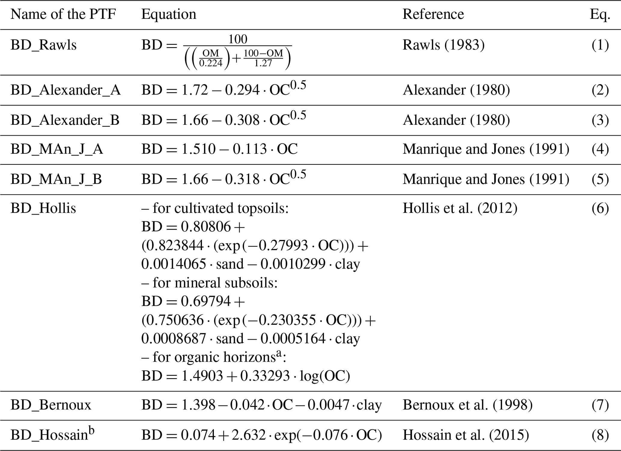
^a For histic and folic horizons which have an organic carbon content equal to or greater than 20 % (IUSS Working Group WRB, 2022). ^b Applied only to organic soils with an organic carbon content equal to or greater than 12 %. OM refers to organic matter content (mass %); OC refers to organic carbon content (mass %); sand refers to sand content (0.05–2 mm fraction) (mass %); band clay refers to clay content (< 0.002 mm fraction) (mass %).

We summarized the information about potential open-access sources for soil information applicable in Europe in Table 1, covering most of the above-listed soil properties. The availability of datasets is continuously improving. The following data sites include most of the updates:

• European Soil Data Centre, which includes soil datasets from Europe and information on the EU Soil Observatory (https://esdac.jrc.ec.europa.eu/, last access: 2 September 2024);

• ISRIC Soil Data Hub, which hosts soil data from around the world (https://data.isric.org/geonetwork/srv/eng/catalog.search#/home, last access: 2 September 2024);

• soil-related layers of the GAEZ Data Portal developed by the Food and Agriculture Organization of the United Nations (FAO) and the International Institute for Applied Systems Analysis (IIASA) (https://data.apps.fao.org, last access: 2 September 2024);

• soil-related layers of the OpenLandMap, which shares open geographical and geoscientific data (https://openlandmap.org, last access: 2 September 2024).

Nevertheless, these sources do not include products from specific institutes, such as http://globalchange.bnu.edu.cn/research, last access: 2 September 2024. The datasets included in Table 1 might be appropriate for regional and continental modelling. However, for catchment-scale and national studies, local and national spatially explicit modelled datasets provide more accurate input information. When a certain local dataset is selected to be used as basic soil information, it is more consistent to compute the missing soil properties from this local data source rather than using other data sources. This allows us to maintain consistency between the different soil properties. For example, it is not recommended to combine local soil property maps at 100 m resolution with soil hydraulic properties retrieved from EU-SoilHydroGrids at 250 m resolution. Where local soil maps with soil layering, organic carbon content, clay, silt, and sand content are available, it is suggested that missing soil properties, such as bulk density, soil hydraulic properties, and albedo, be estimated from the locally available basic soil properties to ensure consistency. The predictions are subject to uncertainty, which depends on the similarity between the training data used for the selected prediction method and the target area in terms of soil physical and chemical characteristics (Román Dobarco et al., 2019; Tranter et al., 2009).

2.1 Evaluation of methods

For soil physical and hydrological properties, the performance of the prediction algorithms was assessed using the European Hydropedological Data Inventory (EU-HYDI), specifically focusing on soil parameters with measured values that are available in the dataset. The EU-HYDI is one of the most comprehensive European soil hydraulic datasets, with soil data of 18 682 samples from 6014 profiles (Weynants et al., 2013). The number of measured values varies according to the soil properties. The EU-HYDI dataset was used to derive hydraulic PTFs, called euptfs. When comparing the performance of a euptf with other methods found in the literature, only the test sets from the EU-HYDI dataset, which were not utilized in the euptf's training, were included. This approach aimed to facilitate a more accurate and fair comparison among different PTFs but decreased the number of samples used for the analysis. The analysis of bulk density prediction was performed on both the EU-HYDI and the LUCAS topsoil dataset (Orgiazzi et al., 2018; Tóth et al., 2013) of 2018. The LUCAS topsoil dataset of 2009 was used for the computation of the nutrient content of the surface soil layer. For the assessment of the topsoil phosphorus maps, we used locally measured data obtained from an agricultural company. This dataset includes soil phosphorus content measured at a depth of 30 cm using the acid ammonium acetate lactate extraction (AL-P) method (Egnér et al., 1960) for 34 agricultural parcels in the year 2009. As the phosphorus content was required according to the Olsen method (Olsen phosphorous or P) (Olsen et al., 1954), we applied the equation of Sárdi et al. (2009) for converting AL-P into Olsen P. Table 2 shows the descriptive statistics of this database.

We compared the algorithms using the mean error (ME), mean absolute error (MAE), root mean squared error (RMSE), Nash–Sutcliffe efficiency (NSE), and coefficient of determination (R²). The non-parametric Kruskal–Wallis test of the R package agricolae (De Mendiburu, 2017) at the 5 % significance level was applied to the squared error values to assess whether there would be significant difference in performance. For soil parameters without measured data in the EU-HYDI dataset, descriptive statistics and histograms of the computed parameters were compared with studies from peer-reviewed literature focused on European applications. The statistical analysis was performed using the R statistics library (R Core Team, 2022).

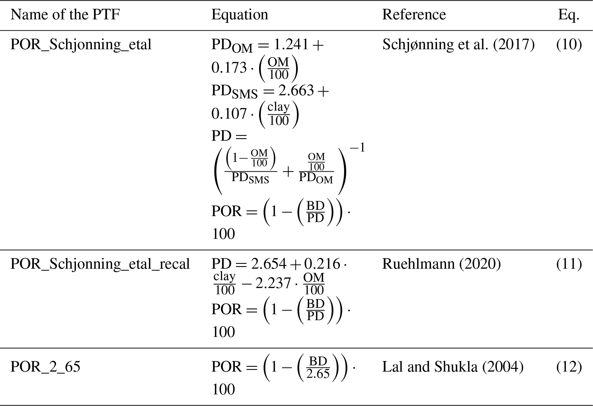
Table 4 List of pedotransfer functions tested based on point data in EU-HYDI for the prediction of porosity.

2.2 Analysed soil properties

We analysed soil physical, hydraulic, and chemical parameters. With regard to the soil physical parameters, we addressed bulk density, porosity, albedo, and soil erodibility factor. For soil hydraulic parameters, we examined water retention, saturated hydraulic conductivity, and hydrological soil groups. Regarding soil nutrient content, we focused on topsoil phosphorus content and described the challenges of retrieving soil nitrate content. Hereinafter, information about the analysis of soil properties is provided.

2.2.1 Soil physical parameters

Bulk density

Table 3 lists the PTFs that were tested based on point data in the EU-HYDI and 2018 LUCAS topsoil datasets. We selected the bulk density PTFs – derived from soils of the temperate region – based on previous works (Casanova et al., 2016; Hossain et al., 2015; Palladino et al., 2022; Xiangsheng et al., 2016) that tested the prediction performance of several methods.

Porosity

Porosity can be computed based on the bulk density and particle density with the following equation:

$$\begin{array}{}\text{(9)}& \mathrm{POR}=\left(\mathrm{1}-\left({\displaystyle \frac{\mathrm{BD}}{\mathrm{PD}}}\right)\right)\cdot \mathrm{100},\end{array}$$

where POR is porosity (volume %), BD is dry bulk density (g cm⁻³), and PD is particle density (g cm⁻³).

As seen in the literature and in SWAT+ model default assumptions (Neitsch et al., 2009), the particle density is usually set to be equal to 2.65 g cm⁻³ (Lal and Shukla, 2004). However, there are PTFs that calculate the porosity based on the particle size distribution (sand, silt, clay content) and organic matter content. We selected the PTFs (Table 4) based on the findings of Ruehlmann (2020) and analysed their prediction performance based on the EU-HYDI dataset.

Note that PD_OM refers to the particle density of the soil mineral substance, PD_MS refers to particle density of the soil organic matter, OM refers to the organic matter content (mass %), sand refers to the sand content (0.05–2 mm fraction) (mass %), and clay refers to the clay content (< 0.002 mm fraction) (mass %).

Albedo

Bare-soil albedo mostly depends on soil moisture variations, surface roughness, soil texture, and organic matter content (Carrer et al., 2014). Time series of soil surface albedo could be retrieved from, for example, the MCD43A3 database or the Copernicus Climate Change Service (2018) (Table 1). If a single characteristic value of soil surface albedo is required for the entire modelling period, such as in the case of the SWAT+ model, the study of Abbaspour et al. (2019) provides several formulas for its computation and suggests substituting the actual volumetric water content with field capacity. For European applications, the equation of Gascoin et al. (2009) could be used:

$$\begin{array}{}\text{(13)}& \mathrm{ALB}=\mathrm{0.31}\cdot \exp \left(-\mathrm{12.7}\cdot \mathit{\theta }\right)+\mathrm{0.15},\end{array}$$

where ALB is soil albedo, and θ is volumetric water content (cm³ cm⁻³), which could be set to the value of the field capacity.

We computed the soil albedo with Eq. (13) for the EU-HYDI topsoil samples, setting the water content to saturation, field capacity, and wilting point. The EU-HYDI dataset does not include the measured soil albedo values at a certain moisture content; therefore, we extracted the median surface albedo for the year 2022 from the MCD43A3 database (https://doi.org/10.5067/MODIS/MCD43A3.061) for two cases: (i) any surfaces throughout the entire year and (ii) only dry, bare soils. We compared the descriptive statistics of computed and mapped values. We considered the visible broadband black-sky albedo for the analysis. Dry bare-soil pixels were selected using the MOD09GA.061 dataset based on the normalized difference vegetation index (NDVI) and the normalized burn ratio 2 (NBR2) indices (Safanelli et al., 2020) in the Google Earth Engine platform (Gorelick et al., 2017) when NDVI values fell in the range of −0.05 and 0.30 and when NBR2 values fell between −0.15 and 0.15. Pixels for dry, bare soils were selected to mask and compare the remotely sensed soil albedo values to the albedo computed at different moisture states.

Soil erodibility factor

The soil erodibility factor (K factor) required for modelling soil erosion can be computed with several methods described in, for example, Kinnell (2010) or Panagos et al. (2014). The most widely used equation that can be readily applied to the most frequently available soil properties was published by Sharpley and Williams (1990) (Eq. 14) and Renard et al. (1997) (Eq. 15). The advantage of these methods is that they require only the sand, silt, clay, and organic carbon content of the soil.

$$\begin{array}{}\text{(14)}& \begin{array}{rl}{K}_{\mathrm{USLE}}& =\left(\mathrm{0.2}+\mathrm{0.3}\cdot \exp \left(\mathrm{0.0256}\cdot \mathrm{sand}\cdot \left(\mathrm{1}-{\displaystyle \frac{\mathrm{silt}}{\mathrm{100}}}\right)\right)\right)\\ & \cdot \left({\left({\displaystyle \frac{\mathrm{silt}}{\mathrm{clay}+\mathrm{silt}}}\right)}^{\mathrm{0.3}}\right)\\ & \cdot \left(\mathrm{1}-\left({\displaystyle \frac{\mathrm{0.25}\cdot \mathrm{OC}}{\left(\mathrm{OC}+\exp \left(\mathrm{3.72}-\mathrm{2.95}\cdot \mathrm{OC}\right)\right)}}\right)\right)\\ & \cdot \left(\mathrm{1}-\left({\displaystyle \frac{\mathrm{0.7}\cdot \left(\mathrm{1}-\frac{\mathrm{sand}}{\mathrm{100}}\right)}{\left(\left(\mathrm{1}-\frac{\mathrm{sand}}{\mathrm{100}}\right)+\exp \left(-\mathrm{5.51}+\mathrm{22.9}\cdot \left(\mathrm{1}-\frac{\mathrm{sand}}{\mathrm{100}}\right)\right)\right)}}\right)\right)\end{array}\end{array}$$

$K_{\mathrm{RUSLE}}=\mathrm{7.594}(\mathrm{0.0034}+\mathrm{0.0405}\cdot \exp (-\mathrm{0.5}\cdot \left(\frac{\log \left(D_{\mathrm{g}}\right)+\mathrm{1659}}{\mathrm{0.7101}}{)}^{\mathrm{2}}\right))$ with

$$\begin{array}{}\text{(15)}& D_{\mathrm{g}}=\exp (\mathrm{0.01}\cdot \sum f_i\cdot \ln m_i)\end{array}$$

In the above, K_USLE is the Universal Soil Loss Equation (USLE), K_RUSLE is the Revised Universal Soil Loss Equation (RUSLE) soil erodibility factor $\left(\frac{\mathrm{t}\cdot \mathrm{arce}\cdot \mathrm{h}}{\text{hundreds of acre}\cdot \text{foot-tonf}\cdot \text{in.}}\right)$, silt is the silt content (mass %, 0.002–0.05 mm), sand is the sand content (mass %, 0.05–2 mm), OC is the organic carbon content (mass %), D_g is the geometric mean particle diameter (mm), f_i is the particle size fraction (mass %), and m_i is the arithmetic mean of the particle size limits of the f_i particle size fraction (mm). If the unit is required in $\left(\frac{\mathrm{t}\cdot \mathrm{ha}\cdot \mathrm{h}}{\mathrm{ha}\cdot \mathrm{MJ}\cdot \mathrm{mm}}\right)$ , the value of the soil erodibility factor computed with Eq. (14) or Eq. (15) has to be multiplied with 0.1317 (Foster et al., 1981).

We computed the soil erodibility factor for the EU-HYDI dataset. Similarly to the above-mentioned albedo, there is no measured soil erodibility value in the EU-HYDI dataset; thus, we compared the values computed for the topsoils of EU-HYDI with the values extracted from the European map of Panagos et al. (2014).

2.2.2 Soil hydraulic parameters

Water retention and saturated hydraulic conductivity

Soil water retention and hydraulic conductivity can be computed from the parameters of the widely used van Genuchten model (VG) (van Genuchten, 1980):

$$\begin{array}{}\text{(16)}& \mathit{\theta }\left(\mathit{\psi }\right)={\mathit{\theta }}_{\mathrm{r}}+{\displaystyle \frac{{\mathit{\theta }}_{\mathrm{s}}-{\mathit{\theta }}_{\mathrm{r}}}{{\left[\mathrm{1}+\left(\mathit{\alpha }{\mathit{\psi }}^n\right)\right]}^m}}\text{with}m=\mathrm{1}-\mathrm{1}/n,\end{array}$$

where θ_r (cm³ cm⁻³) and θ_s (cm³ cm⁻³) are the residual and saturated soil water contents, respectively; α (cm⁻¹) is a scale parameter; and m (–) and n (–) are shape parameters.

Alternative models, like the Kosugi model (Kosugi, 1996), exist for characterizing the water retention curve. However, the availability of predictive tools with which their parameters and equations can derive specific soil hydraulic properties (such as saturated hydraulic conductivity and field capacity based on internal-drainage dynamics) from these parameters is either limited or non-existent (Zhang et al., 2018). Utilizing the VG model to compute all necessary soil hydraulic properties ensures self-consistency of parameters and relies on a dynamic criterion based on soil internal-drainage dynamics (Assouline and Or, 2014; Nasta et al., 2021).

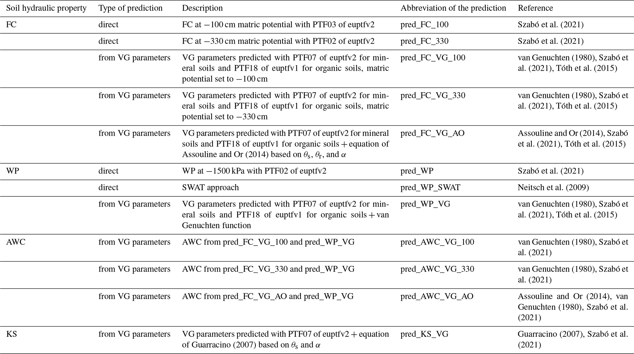
Usually, the FC is considered to be water content at a static soil matric potential. The −330 cm matric potential is widely used for this approximation (Kutiìlek and Nielsen, 1994). Assouline and Or (2014) derived a physically based analytical equation with self-consistent static and dynamic criteria for the prediction of FC. It requires the parameters of the van Genuchten model:

$$\begin{array}{}\text{(17)}& \mathrm{FC}={\mathit{\theta }}_{\mathrm{r}}+\left({\mathit{\theta }}_{\mathrm{s}}-{\mathit{\theta }}_{\mathrm{r}}\right){\left\{\mathrm{1}+{\left[{\displaystyle \frac{n-\mathrm{1}}{n}}\right]}^{\left(\mathrm{1}-\mathrm{2}n\right)}\right\}}^{\left(\frac{\mathrm{1}-n}{n}\right)},\end{array}$$

where FC (cm³ cm⁻³) is water content at field capacity; θ_r (cm³ cm⁻³) and θ_s (cm³ cm⁻³) are the residual and saturated soil water contents, respectively; α (cm⁻¹) is a scale parameter; and n (–) is the shape parameter of the van Genuchten model (van Genuchten, 1980).

Computation of WP could be performed based on the VG parameters using Eq. (18):

$$\begin{array}{}\text{(18)}& \mathrm{WP}={\mathit{\theta }}_{\mathrm{r}}+{\displaystyle \frac{{\mathit{\theta }}_{\mathrm{s}}-{\mathit{\theta }}_{\mathrm{r}}}{{\left[\mathrm{1}+\left(\mathit{\alpha }\cdot {\mathrm{15000}}^n\right)\right]}^{\mathrm{1}-\mathrm{1}/n}}}.\end{array}$$

AWC is defined by FC and WP with the following equation:

$$\begin{array}{}\text{(19)}& \mathrm{AWC}=\mathrm{FC}-\mathrm{WP}.\end{array}$$

Physically, it is impossible to have AWC < 0; therefore, its minimum value has to be set to 0.001 cm³ cm⁻³.

Computation of KS from parameters of the van Genuchten model can be performed by, for example, the equation of Guarracino (2007):

$$\begin{array}{}\text{(20)}& \mathrm{KS}=\mathrm{4.65}\cdot {\mathrm{10}}^{\mathrm{4}}{\mathit{\theta }}_{\mathrm{s}}{\mathit{\alpha }}^{\mathrm{2}},\end{array}$$

where KS is expressed in units of centimetres per day (cm d⁻¹). If a unit in millimetres per hour (mm h⁻¹) is required, the Eq. (20) has to be multiplied by 0.41667.

The most frequently used pedotransfer functions, which can be used to predict soil water content and hydraulic conductivity from easily available soil information, were tested by Nasta et al. (2021) on European datasets: GRIZZLY, HYPRES, and EU-HYDI. Based on their results, we selected the approaches that performed well on the European datasets. Using the selected approaches, we then computed the field capacity (FC), wilting point (WP), plant-available water capacity (AWC), and saturated hydraulic conductivity (KS) for the EU-HYDI dataset. The selected approaches are listed in Table 5. We considered only those approaches which required the mean soil depth, sand, silt, clay content, organic carbon content, and bulk density as input. When FC, WP, AWC, and KS are computed from the measured or predicted parameters of the VG model, the van Genuchten parameters ensure that all required soil hydraulic properties are derived from a physically based model, resulting in a physically plausible soil hydraulic property combination.

Table 5 Approaches tested in the EU-HYDI for the prediction of field capacity (FC), wilting point (WP), available water capacity (AWC), and saturated hydraulic conductivity (KS).

2.2.3 Soil chemical parameters

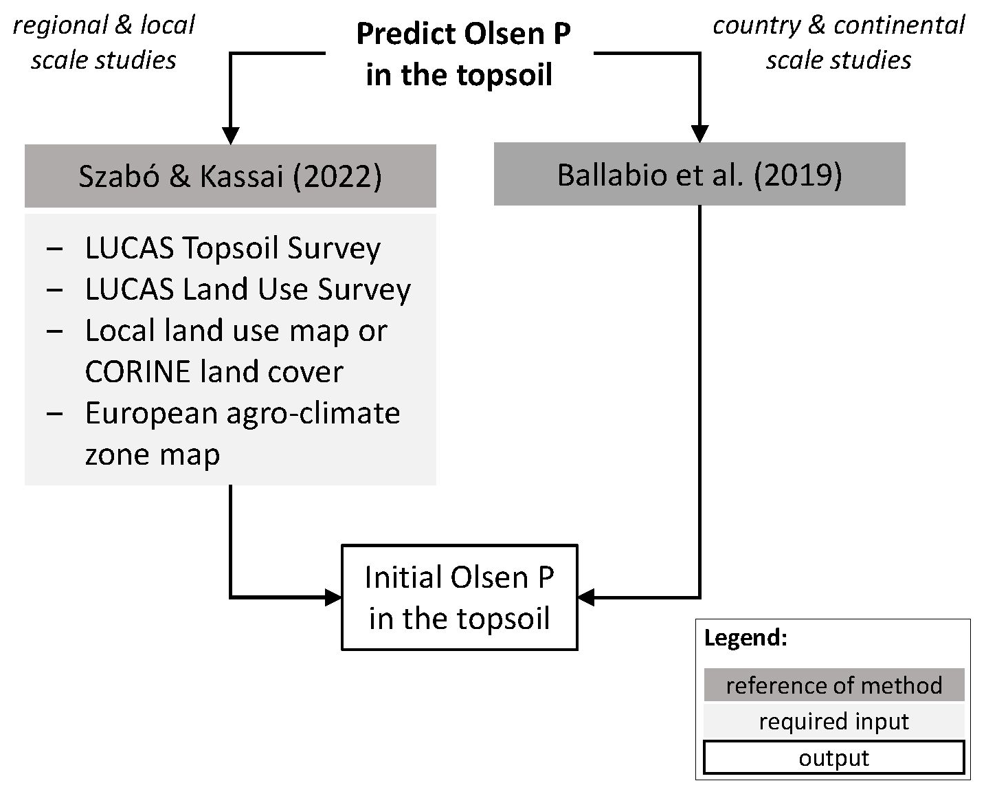
For mapping soil phosphorus (P) content of the topsoil, we present a simple approach based on mean statistics, which is suitable for areas where data are scarce. Land use has the strongest influence on soil P content, with most agricultural areas exhibiting higher P levels compared to regions with natural land cover (Ballabio et al., 2019). The available P level in agricultural soils is influenced by the P inputs – fertilizers, manure, atmospheric deposition, chemical weathering – and outputs – plant uptake and erosion. The agricultural management practices (Tóth et al., 2014) are determined by factors such as the country's economy, climate, tillage practices, and crop production characteristics. Based on the relationships mentioned above, the geometric mean of soil P is computed by land use categories and assigned to the local land use map using the mean statistics-based method. This approach comprises three main steps:

1. First is the selection of LUCAS topsoil samples (EUROSTAT, 2015; Orgiazzi et al., 2018) from the corresponding year and an agro-climatic zone (Ceglar et al., 2019) similar to the target area, preferably in the same country (NUTS region). Additional criteria for the data selection could be comparable soil types and fertilization systems. If this information is not known, the NUTS2 phosphorus map of the European cropland areas might be useful in the data selection (Tóth et al., 2014).

2. Next, we compute the geometric mean of soil P for each land use category.

3. Finally, we assign the mean values to the local land use map.

Further details about the mapping can be found in Szabó and Kassai (2022).

We prepared a soil P content map by applying the proposed method for a case study called Felső-Válicka, located in Hungary (Fig. 1). The resulting map was then compared to (i) the European topsoil phosphorus content map (Ballabio et al., 2019) and (ii) a locally measured independent dataset provided by an agricultural company. Limited availability of soil nutrient data hampered the wider scale of comparison.

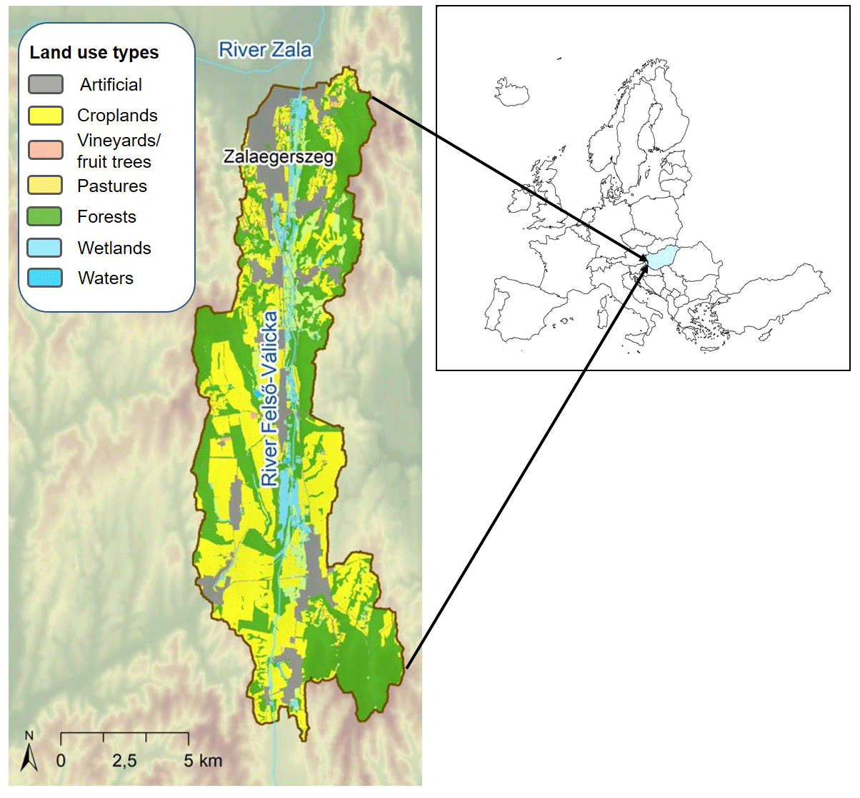
Figure 1 Local land use map of the Felső-Válicka case study in Hungary.

Organic nitrogen can be estimated from soil organic carbon content (Amorim et al., 2022; Liu et al., 2016; Pu et al., 2012; Zhai et al., 2019) if measured data are not available. The concentration of inorganic nitrogen in soil is highly variable in space and time, and the dynamic of its amount is significantly influenced by leaching, denitrification, volatilization, and nitrogen fertilization (Zhu et al., 2021). Therefore, no general method is available for its prediction so far. However, when simulating nitrogen uptake and losses at the catchment scale, information on the amount and timing of nitrogen fertilization is often more crucial than knowledge of the initial nitrate content of the soil (x et al., 2023). The mineral and relatively dynamic N pools are often considered to be initialized during the warm-up period of the models (Yuan and Chiang, 2015). It is especially important to have a proper parameterization of the agricultural management (e.g. fertilization, residue management) setup in the model application, with a warm-up period of appropriate length, which we recommend should be no less than 4 years. Furthermore, it is beneficial to initialize the SOM levels accurately to define the large and rather slow pool of organic nitrogen (Liang et al., 2023).

3 Results and discussion

3.1 Bulk density

Table 6 shows the prediction performance of the selected PTFs. The performance varies depending on the texture classes; e.g. it is lower for clayey soils, sandy clay loams, and loams in the EU-HYDI dataset (Fig. S1a in the Supplement). For the LUCAS topsoil samples, the performance of all PTFs is lower compared to their performance based on EU-HYDI in terms of RMSE. Additionally, all analysed methods tend to overpredict bulk density. The BD_Alexander_A PTF (Eq. 3) ranks highest based on the sample-number-weighted average results of the Kruskal–Wallis test, analysed based on both the EU-HYDI and LUCAS datasets (Table 6, weighted rank). The BD_Alexander_A_Hossain PTF shows the performance of the combined use of the BD_Alexander_ A (for soils with organic carbon content of less than 12 %) and BD_Hossain (for soils with organic carbon content that is equal to or higher than 12 %) PTFs. This combined PTF performs similarly to the simple BD_Alexander_A method but helps to properly derive bulk density for soils with high organic matter content. Figure 2 shows the scatterplot of the measured versus predicted bulk density values of the best-performing PTF, where the predefined bulk density is capped at 1.72 g cm⁻³ as a product of the models constraints.

Table 6 Prediction performance of bulk density (g cm⁻³) computed using available pedotransfer functions based on the point data of EU-HYDI (N=11 273) and LUCAS (N=5821). ME refers to the mean error, MAE refers to the mean absolute error, RMSE refers to the root mean squared error, NSE refers to the Nash–Sutcliffe efficiency, and R² refers to the coefficient of determination.

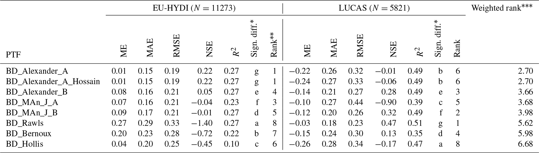
^* Different letters indicate significant differences at the 0.05 level between the accuracy of the methods based on the squared error; for example, performance indicated with the letter c is significantly better than the one noted with the letters b and a. ${}^{**}$ Rank based on the Kruskal–Wallis test; 1 denotes the best-performing method. ${}^{***}$ Sample-number-weighted average results of the Kruskal–Wallis test.

If only the soil's organic carbon content is known, the prediction accuracy is restricted. The RMSE value of BD_Alexander_A_Hossain PTF based on the EU-HYDI is comparable with the accuracy of an ML-based PTF built on a French dataset (Chen et al., 2018) when computed based on independent validation sets, which reported RMSE values between 0.17 and 0.22 g cm⁻³. This performance is better than the results of a model transferability test of a PTF derived from soils from Campania, Italy, analysed based on the EU-HYDI (Palladino et al., 2022), which had an RMSE of 0.210 g cm⁻³. Xiangsheng et al. (2016) and De Souza et al. (2016) found RMSE values higher than 0.185 g cm⁻³ when they applied PTFs trained on temperate soils, available from the literature, to a Chinese permafrost region and to a Brazilian catchment, respectively. This outcome underscores the significance of refraining from using a PTF that was trained on soils formed under different conditions (i.e. with different soil forming factors), making it inapplicable to the specific target area (Chen et al., 2018; Tranter et al., 2009).

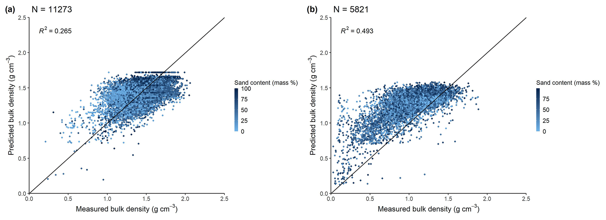
Figure 2 Scatterplot of measured versus predicted bulk density values of the best-performing PTF (BD_Alexander_ A_Hossain) analysed based on the point data of the EU-HYDI (a) and LUCAS (b) datasets.

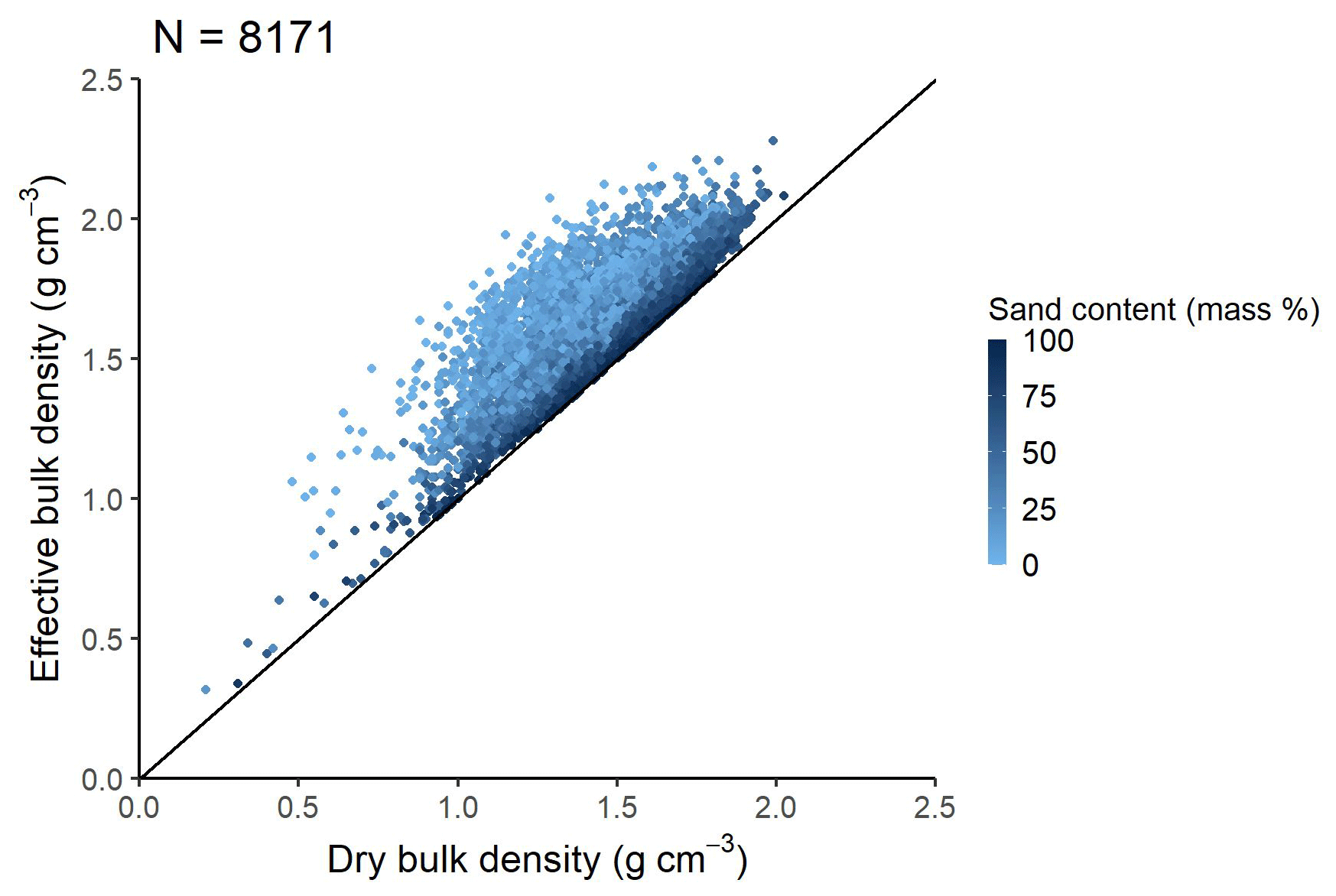
Figure 3 Scatterplot of dry versus effective bulk density analysed based on the point data of EU-HYDI.

Effective bulk density is always higher than dry bulk density. The effective bulk density value computed for the EU-HYDI dataset with Eqs. (22) and (23) was between 0.32 and 2.17 g cm⁻³. Figure 3 shows the scatterplot of dry bulk density versus computed effective bulk density based on the EU-HYDI dataset.

Based on the performance analysis on EU-HYDI (N=11 273), the prediction of dry bulk density could be performed with (i) Eq. (2) (BD_Alexander_A) for soils with OC < 12 % and (ii) Eq. (8) (BD_Hossain) for soils with OC > = 12 %.

3.2 Porosity

The porosity values computed based on the particle density predicted by Schjønning et al. (2017) (PTF (POR_Schjonning_etal) implemented in Eq. (10)) were significantly more accurate for those EU-HYDI samples, which considered the measured particle density value for the computation of porosity (Table 7). If solely samples with low organic matter content, specifically less than 1 %, were considered for analysis, no notable differences between the methods were observed. In the case of soils with organic matter content higher than 1 %, the prediction of porosity significantly improved if particle density was computed based on the distinction between organic matter and mineral substrates. Figure 4 displays the scatterplot of measured versus predicted (Eq. (10) – POR_Schjonning_etal) porosity values.

Table 7 Prediction performances of porosity (vol %) computed using available pedotransfer functions based on the point data of EU-HYDI results are structured by organic matter content. OM refers to organic matter content (mass %), N refers to the number of samples, ME refers to the mean error, MAE refers to the mean absolute error, RMSE refers to the root mean squared error, NSE refers to the Nash–Sutcliffe efficiency, and R² refers to the coefficient of determination.

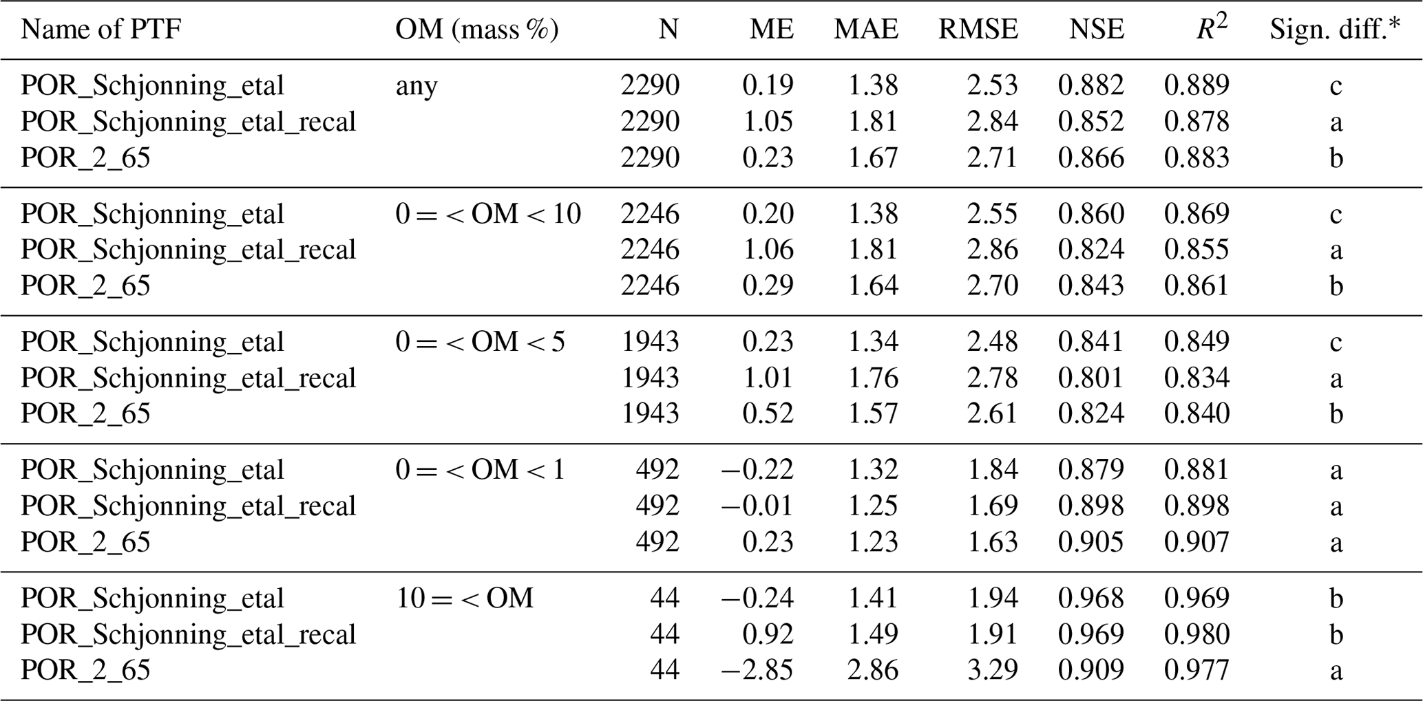
^* Different letters indicate significant differences at the 0.05 level between the accuracy of the methods based on the squared error; for example, performance indicated with the letter c is significantly better than the one noted with letters b and a.

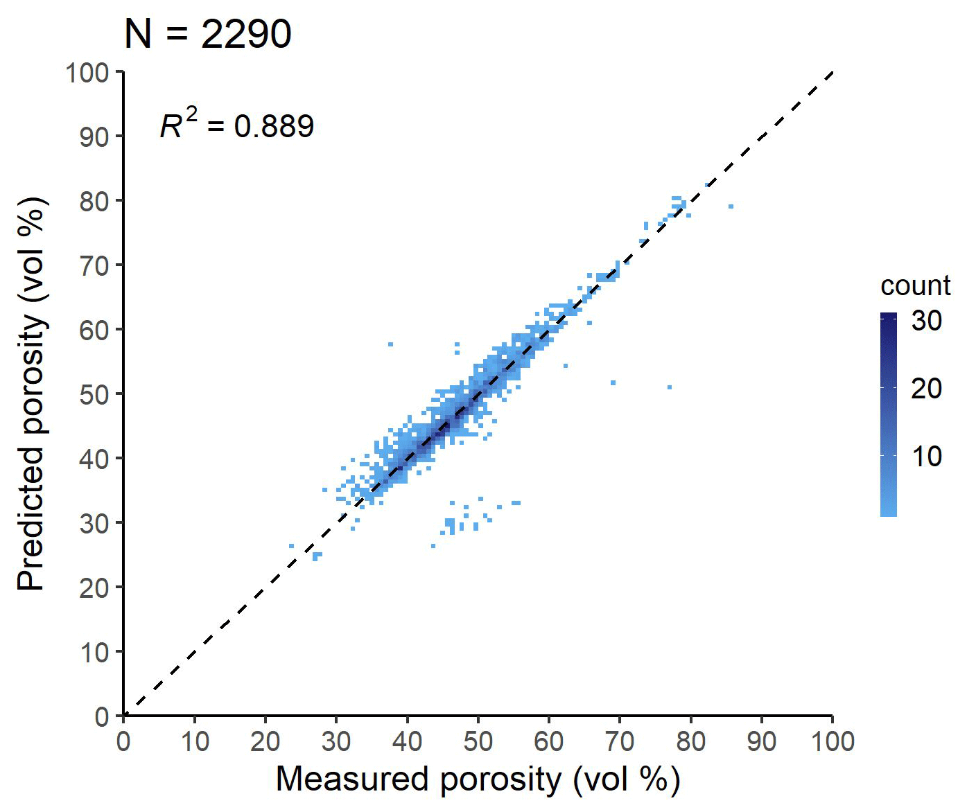
Figure 4 Scatterplot of measured versus predicted porosity values of the best-performing PTF, POR_Schjonning_etal (Eq. 10), analysed based on the EU-HYDI subset with measured particle density values. Count refers to the number of cases in each quadrangle.

When data on porosity are missing, some studies use the saturated water content as its approximation, although, based on the literature, the saturated water content is usually equal to or less than the total porosity (Lal and Shukla, 2004). Figure 5 shows the relationship between porosity and saturated water content for 391 EU-HYDI samples with measured values of both parameters. Among these samples, 56.5 % have a total porosity larger than or equal to the saturated water content. For the samples where the saturated water content is higher than the total porosity, the reason may be the uncertainties in the measurement of both parameters. It is possible that free water could have pounded on top of the sample when its saturated weight was measured, and errors in the measurement of particle density used to compute porosity may have also contributed (Kutiìlek and Nielsen, 1994; Nimmo, 2004), resulting in a lower porosity.

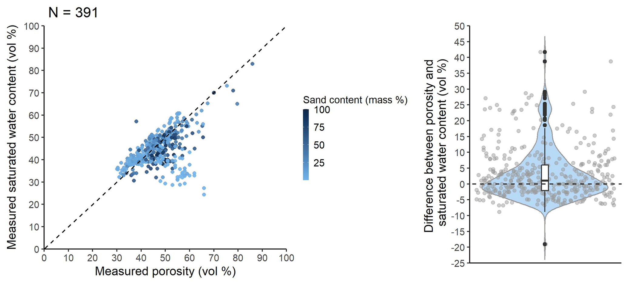
Figure 5 Scatterplot of measured porosity values versus measured saturated water content and boxplot of the difference between the two values tested on point data in the EU-HYDI dataset.

Based on the study performed in EU_HYDI, prediction of porosity could be performed with the Schjønning et al. (2017) PTF of Eq. (10) instead of defining particle density as 2.65 g cm⁻³, as in Eq. (12).

3.3 Albedo

The range of soil albedos computed with Eq. (13) for the topsoil layers of the EU-HYDI dataset with different moisture states (Table 8) is within the range of the values available from the literature, which is 0.10–0.43 in the case of the ECOCLIMAP-U dataset (Carrer et al., 2014). The median albedo of dry, bare soil and the surface albedo values of the year 2022 extracted from the MCD43A3 database to the EU-HYDI topsoil layers are significantly lower than the computed values (Fig. 6). The histograms of the monthly values of surface albedo and dry, bare soil albedo extracted to the EU-HYDI topsoil samples are show in Fig. S2a and b. It is crucial to specify the moisture condition for which the albedo value is needed in the modelling process.

Table 8 Descriptive statistics of soil albedo values computed with the simplified Gascoin et al. (2009) equation for the topsoil samples of the EU-HYDI dataset (N=7537) at different moisture states: based on saturation (ALB_comp_THS), field capacity (ALB_comp_FC), and wilting point (ALB_comp_WP).

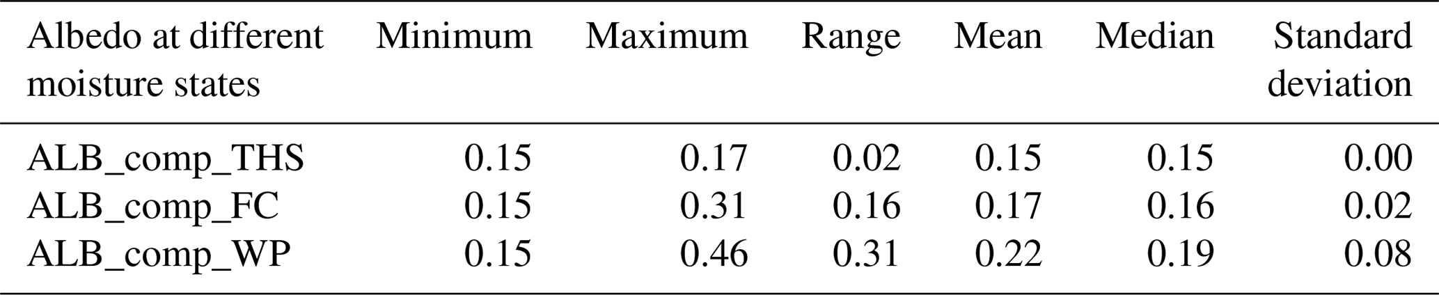
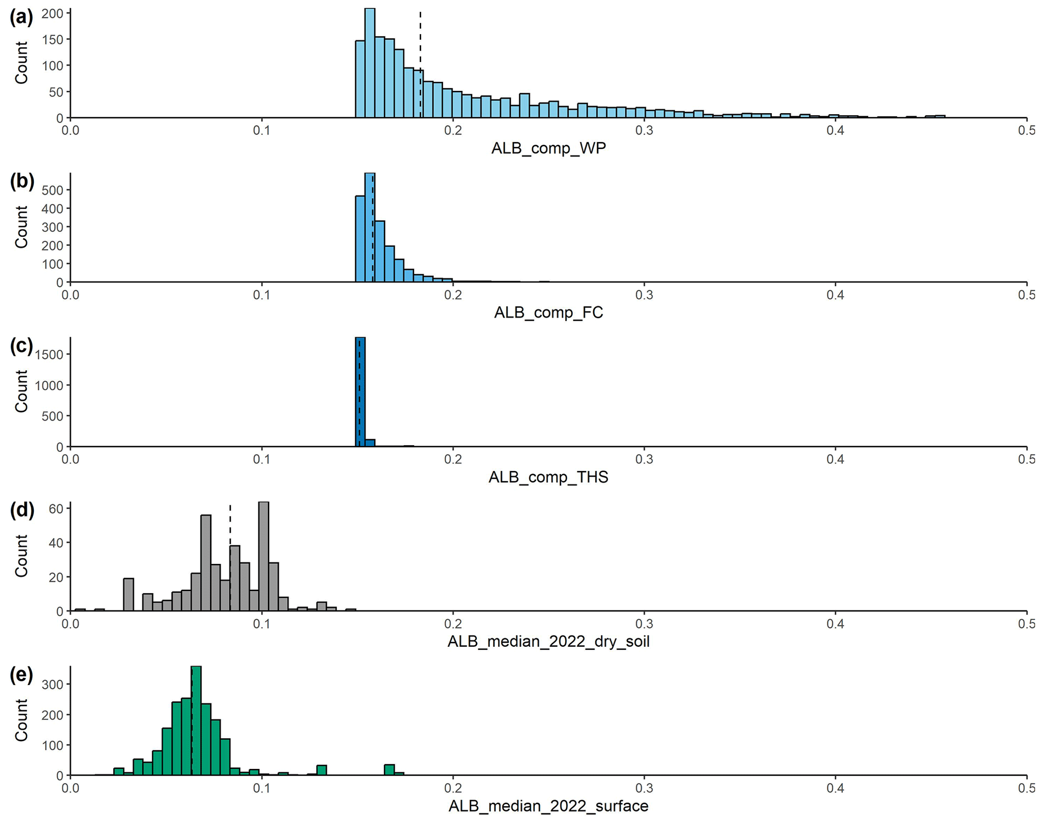
Figure 6 Histograms of the soil albedo computed with the Gascoin et al. (2009) equation for the topsoil layers of the EU-HYDI dataset in the case of three moisture states: at saturation (ALB_comp_THS) (a), internal-drainage-dynamics-based field capacity (ALB_comp_FC) (b) and wilting point (ALB_comp_WP) (c) (N=2408), and median surface albedo (d) and albedo of dry, bare soil (e) for the year 2022 (ALB_median_2022_dry_soil, ALB_median_2022_surface) extracted from the MCD43A3 global database for the EU-HYDI topsoil layers. Vertical dashed lines indicate the median values.

3.4 Soil erodibility factor

The soil erodibility factor (K factor) computed based on the topsoil samples of the EU-HYDI dataset with Eq. (14) are comparable to the values of the European 500 m resolution soil erodibility map published by Panagos et al. (2014) in terms of the range, mean, and density of the values (Table 9 and Fig. 7), although the relationship between the computed and mapped values was weak (Fig. 8). For the computation of the European soil organic matter content map, soil texture, coarse-fragment content, soil structure, and stoniness were considered. The Renard et al. (1997) (Eq. 15) equation resulted in a higher median value but a lower possible maximum value because the computed soil erodibility factor is capped at 0.044 $\left(\frac{\mathrm{t}\cdot \mathrm{ha}\cdot \mathrm{h}}{\mathrm{ha}\cdot \mathrm{MJ}\cdot \mathrm{mm}}\right)$ due to the constraints of the model. The relationship between the soil erodibility factors derived by different methods is strongest between the values computed using the Sharpley and Williams (1990) method and the Renard et al. (1997) method. This is logical because both methods consider the particle size distribution of the soil as input information.

Both approaches, whether directly applying the equations (Eqs. 14 or 15) or extracting values, generate predicted soil erodibility values. While both can be used for environmental modelling, (i) the European soil erodibility map could be linked with the LUCAS topsoil dataset and maps, and (ii) employing Eqs. (14) or (15) might offer greater consistency with the other local basic and physical soil data, aligning more seamlessly with the modelling process. Given the scarcity of measured K-factor values, our suggestion is to initially utilize these predicted values as preliminary approximations. However, we recommend fine-tuning this factor during the model calibration process.

Table 9 Descriptive statistics of soil erodibility factor values computed with the Sharpley and Williams (1990) and Renard et al. (1997) equations based on the topsoil samples of the EU-HYDI dataset (N=11 287) provided in US customary units $\left(\frac{\mathrm{t}\cdot \mathrm{arce}\cdot \mathrm{h}}{\text{hundreds of acre}\cdot \text{foot-tonf}\cdot \text{in.}}\right)$ and SI units $\left(\frac{\mathrm{t}\cdot \mathrm{ha}\cdot \mathrm{h}}{\mathrm{ha}\cdot \mathrm{MJ}\cdot \mathrm{mm}}\right)$.

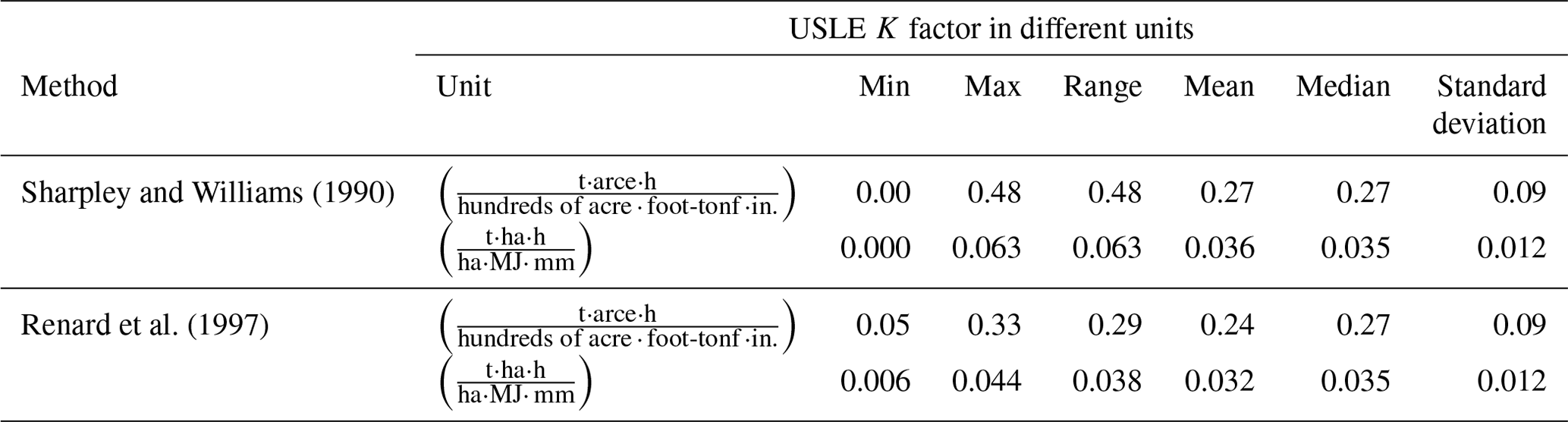
Figure 7 Histogram of the soil erodibility factor $\left(\frac{\mathrm{t}\cdot \mathrm{ha}\cdot \mathrm{h}}{\mathrm{ha}\cdot \mathrm{MJ}\cdot \mathrm{mm}}\right)$ computed with the Sharpley and Williams (1990) (K_Sharpley_Williams, N=3276) (a) and Renard et al. (1997) (K_Renard, N=3276) (b) equations based on the topsoil samples of the EU-HYDI dataset and extracted from the soil erodibility map of Europe for the EU-HYDI topsoil layers without considering stoniness (K_ESDAC, N=3100), (c) and considering stoniness (K_st_ESDAC, N=3190) (d). Vertical dashed lines indicate the median values.

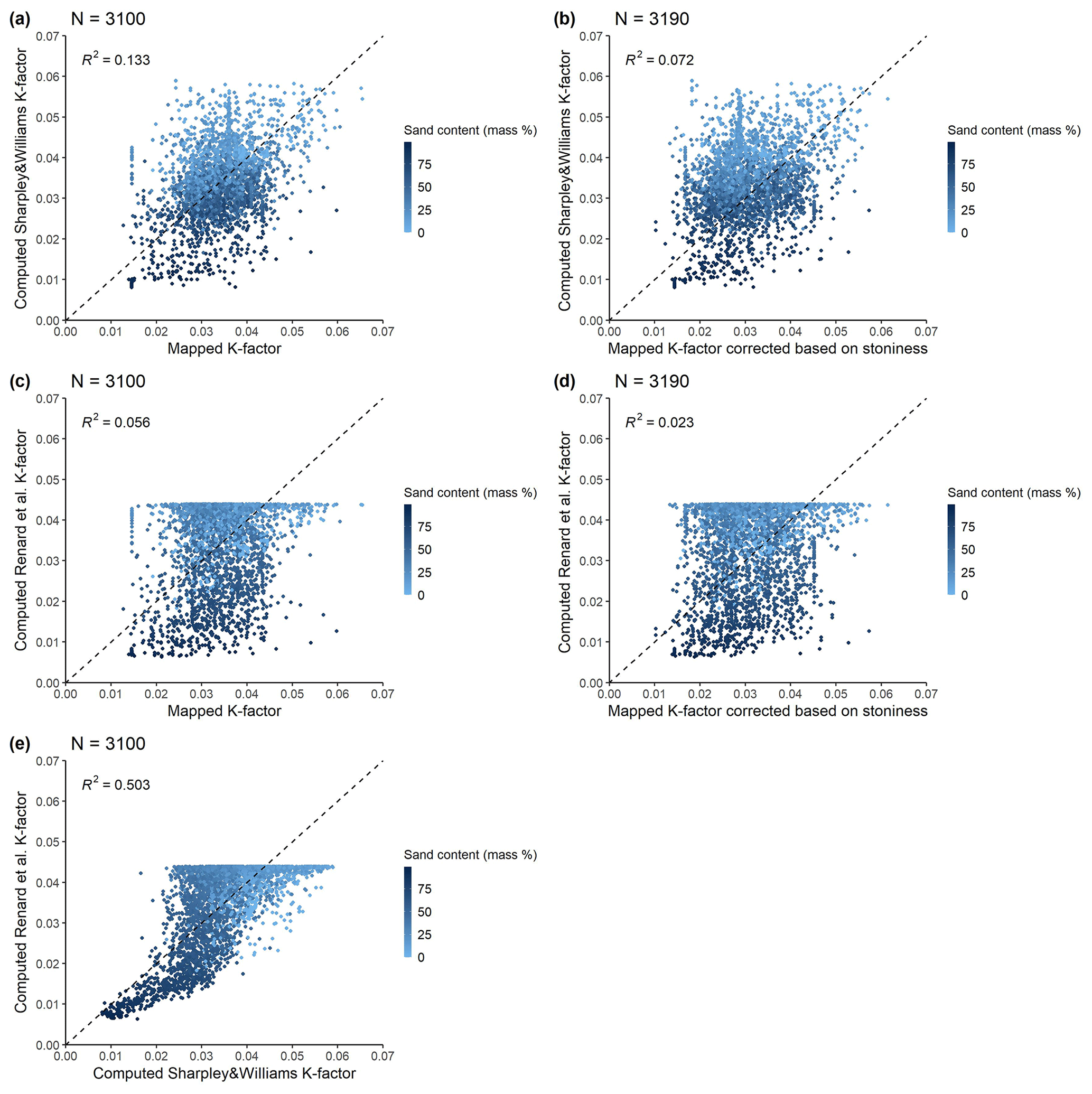
Figure 8 Scatterplot of computed soil erodibility factors versus those extracted from the European soil erodibility factor map without (a, c) and with stoniness (b, d) based on the topsoil samples of the EU-HYDI dataset $\left(\frac{\mathrm{t}\cdot \mathrm{ha}\cdot \mathrm{h}}{\mathrm{ha}\cdot \mathrm{MJ}\cdot \mathrm{mm}}\right)$. Plot (e) shows the relationship between the values computed by the Sharpley and Williams (1990) and Renard et al. (1997) methods.

3.5 Field capacity

The FC defined (see abbreviations in Table 5) based on soil internal-drainage dynamics (FC_VG_AO) differed from the field capacity measured at −100 cm, or −330 cm matric potential (FC_100 and FC_330, respectively) or computed from VG parameters at −100 cm or −330 cm matric potential (FC_VG_100 and FC__VG_330, respectively) (Fig. 9), as was expected. The scale of difference depends on (i) the predefined soil matric-potential value, which we consider using as the measured field capacity, and (ii) characteristic soil properties that influence soil hydraulic behaviour, such as soil texture, organic matter content, bulk density, clay mineralogy, and structure. Figures S3 and S4 show that, for soils with low sand content (< 25 %) and high silt content (> 50 %) or low bulk density (< 0.7 g cm⁻³), the FC_ VG_AO is lower than the water content measured at −100 cm or −330 cm matric potential (FC_VG_AO vs. FC_100 and FC_VG_AO vs. FC_330).

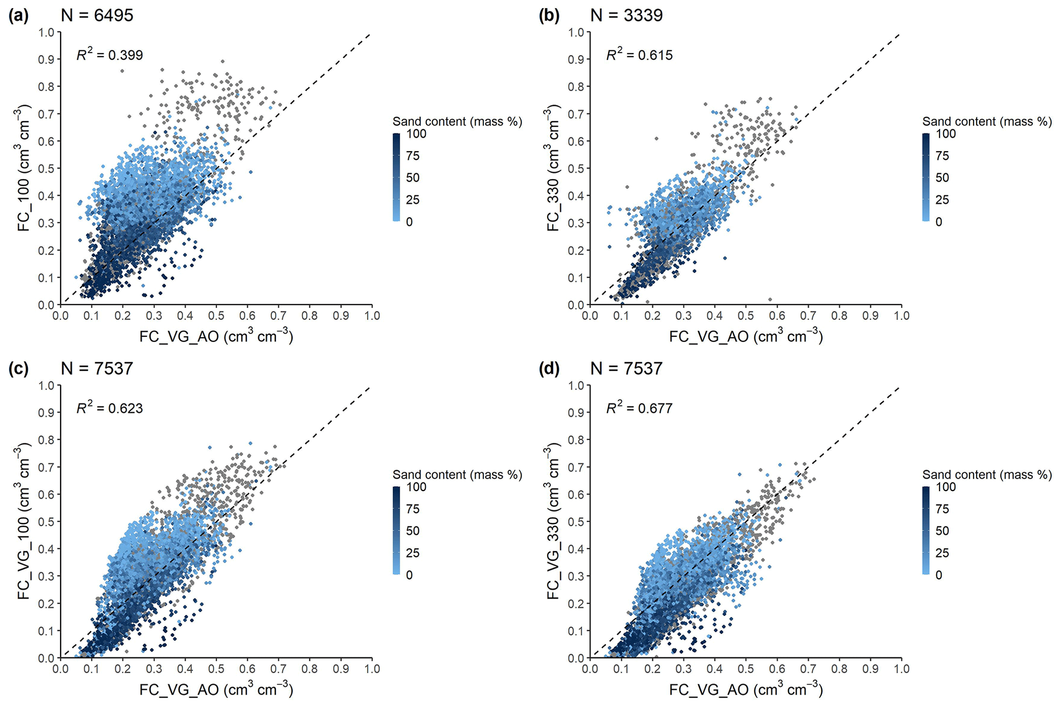
Figure 9 Scatterplot of internal-drainage-dynamics-based field capacity (FC_VG_AO) versus field capacity at −100 cm matric potential (a) and at −330 cm matric potential (b), computed based on VG model with parameter h (head) set at −100 cm matric potential (c) and −330 cm matric potential (d).

If FC at a single matric-potential value is computed from the fitted VG parameters (FC_VG_100, FC_VG_330), their Pearson correlation with the FC_VG_AO is higher than in the case of FC measured at −100 or −330 cm matric potential (Fig. S5). This is logical because, in the case of FC_VG_100 and FC_VG_300, the same VG parameters are used for the computation as for FC_VG_AO. In the case of EU-HYDI, the FC_VG_330 is the closest to the FC_VG_AO. The only exception are sands where FC measured at −330 cm matric potential has the highest correspondence with FC_VG_AO (Fig. S6).

Table 10 Prediction performance of internal-drainage-dynamics-based field capacity (cm³ cm⁻³) computed by pedotransfer functions based on the FC and VG test sets of the EU-HYDI dataset. N refers to the number of samples, ME refers to the mean error, MAE refers to the mean absolute error, RMSE refers to the root mean squared error, NSE refers to the Nash–Sutcliffe efficiency, and R² refers to the coefficient of determination.

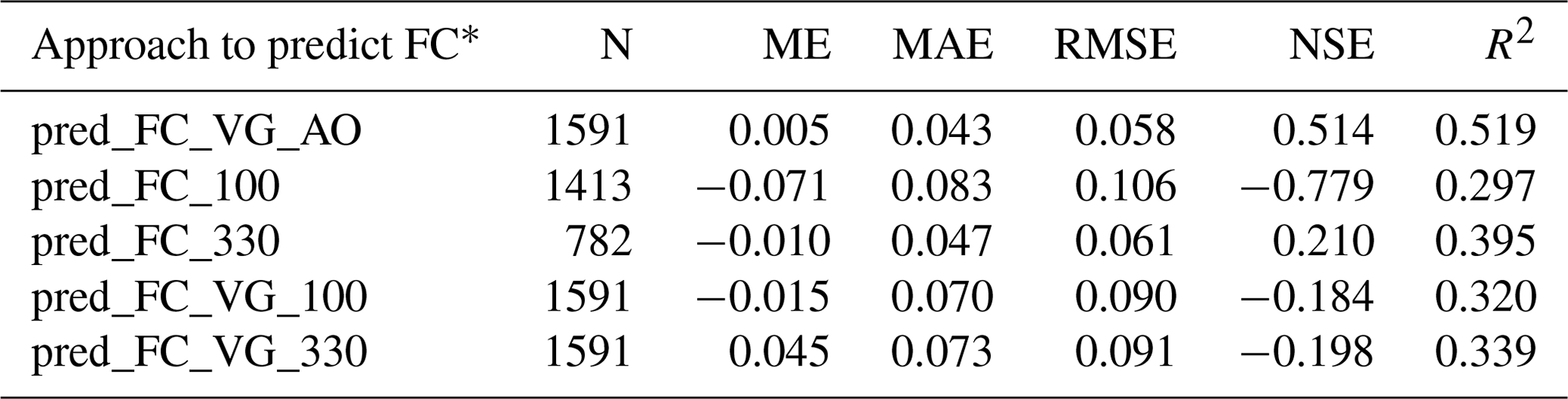
^* pred_FC_VG_AO is the predicted internal-drainage-dynamics-based field capacity based on VG parameters predicted from basic soil properties, pred_FC_100, pred_ FC_ 330 is the field capacity at −100 and −330 cm matric potential directly predicted from basic soil properties, and pred_FC_VG_100 and pred_FC_VG_330 are field capacity at −100 and −330 cm matric potential based on VG parameters predicted from basic soil properties.

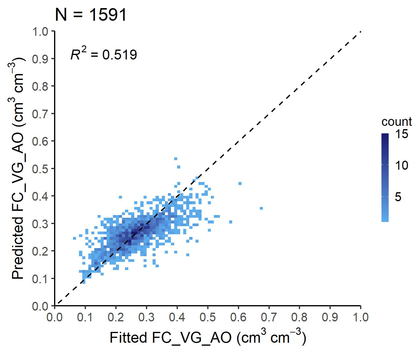
Figure 10 Scatterplot of internal-drainage-dynamics-based FC (FC_VG_AO) computed from fitted and predicted VG parameters analysed based on the VG test set of the EU-HYDI dataset. Count refers to the number of cases in each quadrangle.

Table 10 illustrates the prediction performance of the FC_VG_ AO for various approaches. If the FC_VG_AO was computed based on VG parameters predicted by the PTF07 of euptfv2, the RMSE value was 0.058 cm³ cm⁻³, which is comparable with the literature values (Román Dobarco et al., 2019; Zhang and Schaap, 2017). Its correlation with the FC computed based on predicted VG parameters at −100 or −330 cm matric potential is weaker (with RMSE values of 0.090 and 0.091 cm³ cm⁻³), aligning with the results drawn from the FC computed from fitted VG parameters (Fig. 9c and d).

Figure 10 shows the scatterplot of FC_VG_AO computed from fitted and predicted VG parameters, analysed based on only those samples of the EU-HYDI which were not used for training of the VG PTF07. The performance of VG PTF07 was published in Szabó et al. (2021), with 0.054 cm³ cm⁻³ RMSE for the test set.

Thus FC_VG_AO could be used as FC and can be computed with Eq. (17) based on VG parameters predicted with (i) euptfv2 (Szabó et al., 2021) for mineral soils and (ii) euptfv1 (Tóth et al., 2015) class PTF (PTF18) for organic soils.

3.6 Wilting point

Calculating WP (see abbreviations in Table 5) from predicted VG parameters yields greater accuracy compared to using the equation provided by the SWAT+ model (Fig. 11, Table 11). Predicting WP directly from soil properties instead of deriving it from predicted VG parameters tends to yield greater accuracy (Børgesen and Schaap, 2005; Szabó et al., 2021; Tomasella et al., 2003) (Table 12). When multiple soil hydraulic parameters are needed, deriving all of them from a model encompassing the entire matric-potential range secures the physical relationship between them (Weber et al., 2024).

Table 11 Prediction performance of wilting point (cm³ cm⁻³) derived with the VG model, computed using pedotransfer functions based on the VG test set of the EU-HYDI dataset. Observed variable is the WP value computed based on the fitted parameters of the VG model. N refers to the number of samples, ME refers to the mean error, MAE refers to the mean absolute error, RMSE refers to the root mean squared error, NSE refers to the Nash–Sutcliffe efficiency, and R² refers to the coefficient of determination.

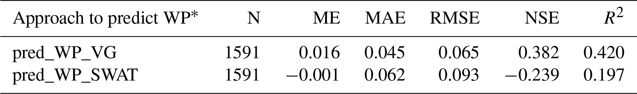
^* pred_WP_VG is the wilting point computed based on VG parameters predicted from basic soil properties, and pred_WP_ SWAT is the wilting point predicted with the equation built into the SWAT model.

Table 12 Prediction performance of wilting point (cm³ cm⁻³) computed by pedotransfer functions based on the WP test set of the EU-HYDI dataset. Observed variable is the measured WP value. N refers to the number of samples, ME refers to the mean error, MAE refers to the mean absolute error, RMSE refers to the root mean squared error, NSE refers to the Nash–Sutcliffe efficiency, and R² refers to the coefficient of determination.

^* pred_WP_VG is the wilting point computed based on VG parameters predicted from basic soil properties, pred_WP_ SWAT is the wilting point predicted with the equation built into the SWAT model, and pred_WP is the wilting point directly predicted from basic soil properties.

WP could be computed with Eq. (18) based on VG parameters predicted with (i) euptfv2 (Szabó et al., 2021) for mineral soils and (ii) euptfv1 (Tóth et al., 2015) class PTF (PTF18) for organic soils.

3.7 Available water capacity

If only AWC (see abbreviations in Table 5) is required as input for a model, i.e. without FC and WP, a feasible option could involve direct prediction using a PTF like euptfv2. However, its estimation is more accurate if the internal-drainage-dynamics-based FC is considered for its computation (Gupta et al., 2023). Figures 12 and S9 show that the coefficient of determination is low between the internal-drainage-dynamics-based AWC (AWC_VG_AO) and AWC based on FC at a fixed matric potential (AWC_100, AWC_300, AWC_VG_100, AWC_VG_330). Which approach is the closest to the AWC_VG_AO varies based on texture classes (Fig. S10).

The available water capacity based on field capacity measured at a −100 cm head (AWC_100) is higher than the AWC_VG_AO, especially in the case of low sand content (< 25 %) and high silt content (> 50 %) (Figs. 12c and S7). The available water capacity based on field capacity measured at a −330 cm head (AWC_330) is higher than AWC_AO_VG when sand content is low (< 25 %) and when silt content is high (> 50 %) and is lower than AWC_AO_VG when sand content is higher than 25 % and when silt content is less than 50 % (Figs. 12d and S8).

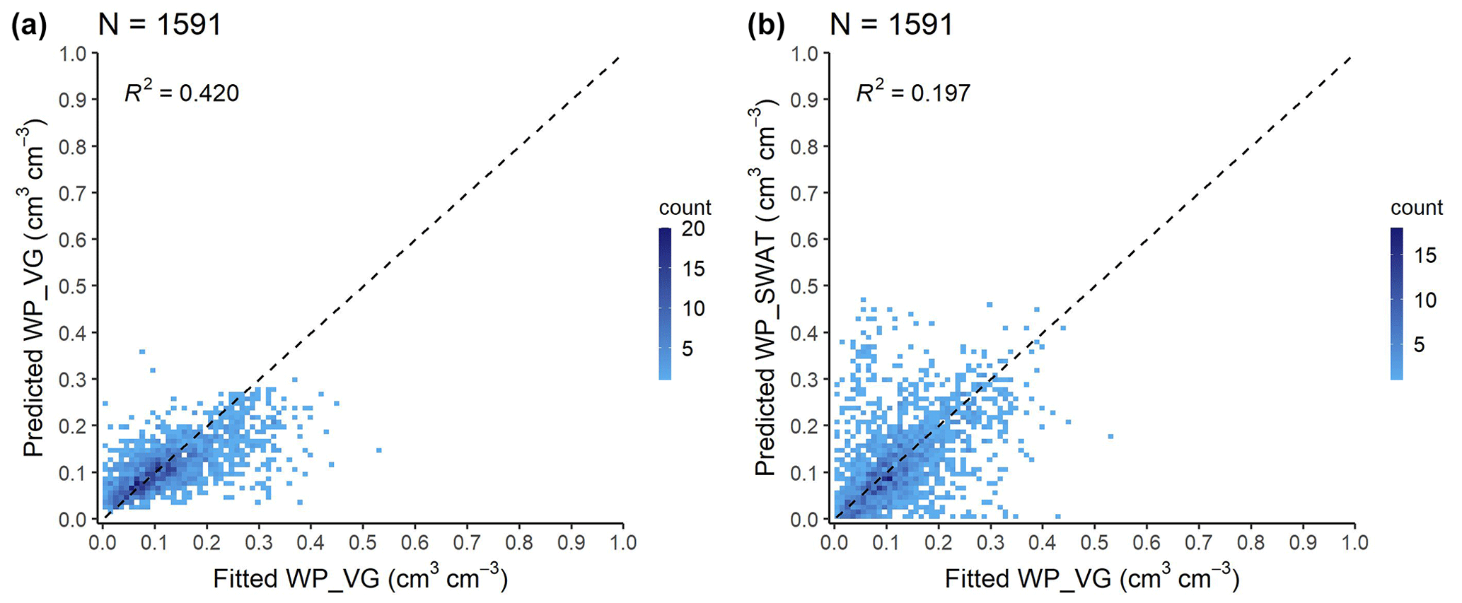
Figure 11 Scatterplot of wilting point computed from fitted VG parameters (Fitted WP_VG) versus (a) wilting point computed from VG parameters predicted with euptfv2 (Predicted WP_VG) and (b) wilting point predicted with the SWAT+ approach (Predicted WP_SWAT), analysed based on the VG test set of the EU-HYDI dataset. Count refers to the number of cases in each quadrangle.

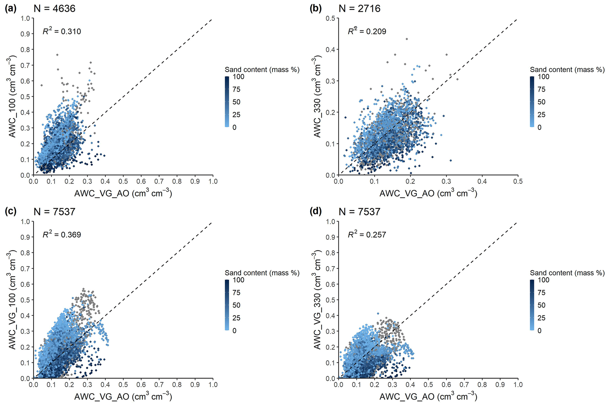
Figure 12 Scatterplot of available water capacity computed from internal-drainage-dynamics-based field capacity and wilting point derived based on VG parameters predicted from basic soil properties (AWC_VG_AO) versus (a, b) available water capacity computed from measured field capacity at −100 and−330 cm matric potential and wilting point and (c, d) available water capacity computed from field capacity at −100 and −330 cm matric potential and wilting point based on VG parameters predicted from basic soil properties.

Table 13 Prediction performance of available water capacity (cm³ cm⁻³) computed by pedotransfer functions based on the VG test set of the EU-HYDI dataset. N refers to the number of samples, ME refers to the mean error, MAE refers to the mean absolute error, RMSE refers to the root mean squared error, NSE refers to the Nash–Sutcliffe efficiency, and R² refers to the coefficient of determination.

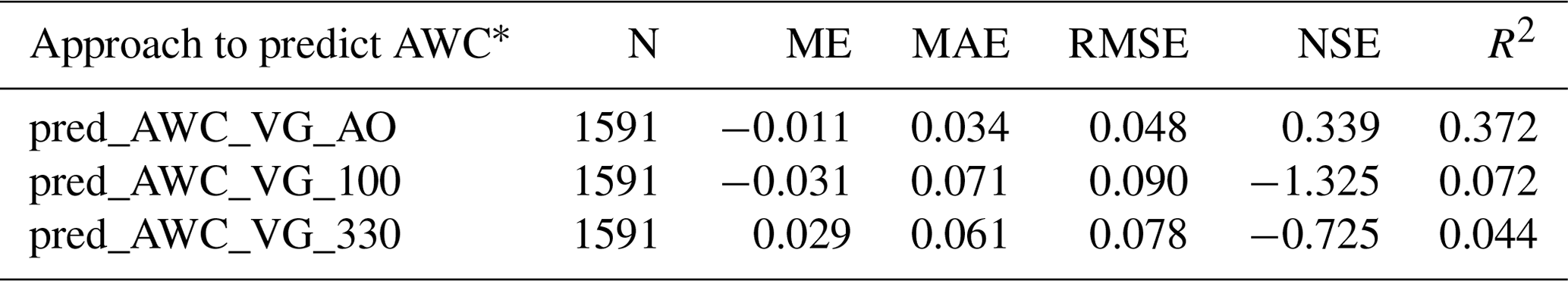
^* pred_AWC_VG_AO is the available water capacity computed from internal-drainage-dynamics-based field capacity and wilting point derived based on VG parameters predicted from basic soil properties, and pred_AWC_VG_100 and pred_AWC_VG_330 are the available water capacity computed from field capacity at −100 and −330 cm matric potential and wilting point based on VG parameters predicted from basic soil properties.

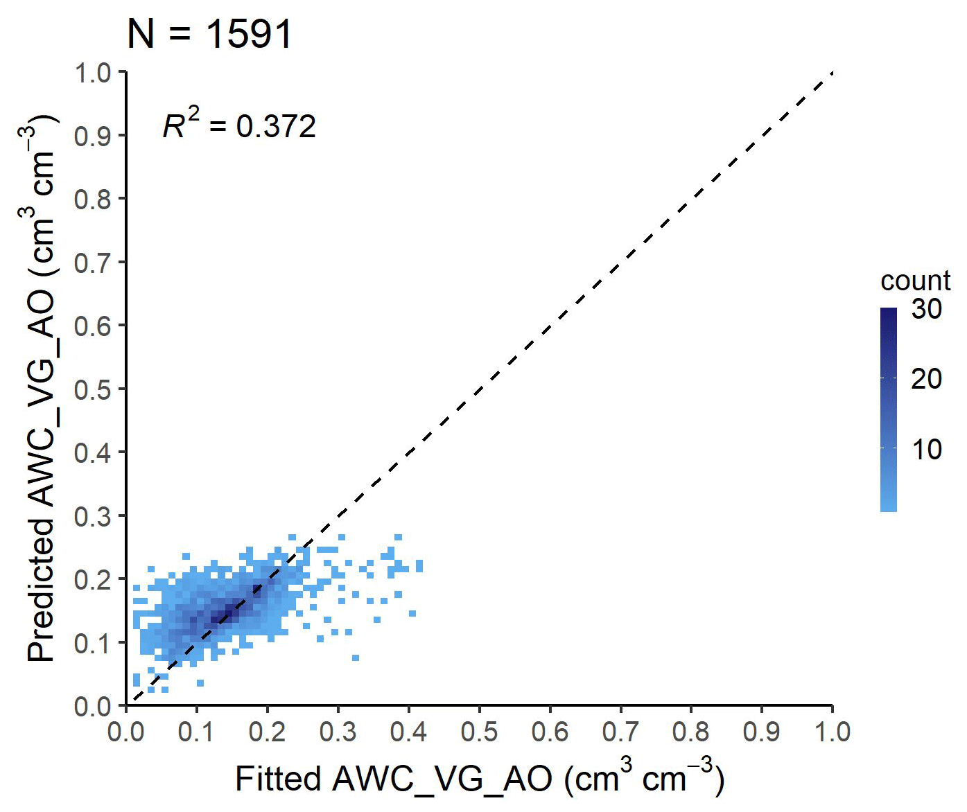
Figure 13 Scatterplot of internal-drainage-dynamics-based AWC (AWC_VG_AO) computed from fitted and predicted VG parameters analysed based on the VG test set of the EU-HYDI dataset. Count refers to the number of cases in each quadrangle.

Table 13 shows the prediction performance of internal-drainage-dynamics-based AWC (AWC_VG_AO). As expected, the predicted internal-drainage-dynamics-based AWC had the lowest RMSE and the highest R² value. The AWC computed based on the FC at 100 cm matric head derived with the predicted VG parameters (pred_AWC_ VG_ 100) had the lowest performance. This approach yielded over-prediction of the AWC_VG_AO values when AWC_VG_AO was lower than 0.10 cm³ cm⁻³ and yielded under-prediction when AWC_VG_AO was higher than 0.25 cm³ cm⁻³ (Fig. 13).

Based on the findings, we recommend computing the AWC based on the internal-drainage-dynamics-based FC (FC_VG_AO) and VG-parameter-based WP (WP_VG) in Eq. (19).

3.8 Saturated hydraulic conductivity

Figure 14 shows the relationship between measured KS and that computed with Eq. (20) based on the fitted VG parameters (KS_VG) (see abbreviation in Table 5). The coefficient of determination between the measured and computed values is low; however, fitted (not predicted) VG parameters were used for the computation. The prediction performance of KS_VG is comparable with the widely used published PTFs (Nasta et al., 2021) (Fig. 15, Table 14).

Prediction of saturated hydraulic conductivity (KS) has the highest uncertainty among the soil hydraulic properties. This uncertainty originates from the differences in the measurement methods applied to measuring KS in terms of sampling volume, sample dimensions, and differences between in situ and laboratory methods (Ghanbarian et al., 2017). Due to the uncertainty of the measurements, the uncertainty of the prediction is, at minimum, 1 order of magnitude during the application of a PTF (Nasta et al., 2021). The estimation of KS by traditional PTFs that use basic soil properties as input is rather limited because the KS of a sample is largely determined by its structural properties and pore network characteristics, of which we lack quantitative descriptors and data (Lilly et al., 2008). There is also at least 1-order-of-magnitude difference between replicated measurements of samples coming from the same soil horizon due to the extreme spatial variability of this particular soil property. Hence, it is important to note that, while we might improve individual sample predictions for KS, the representativeness of these samples within their specific fields remains constrained. We suggest initializing this soil property using the VG parameters with Eq. (20) but keeping in mind that it should be adjusted during model calibration as a variable.

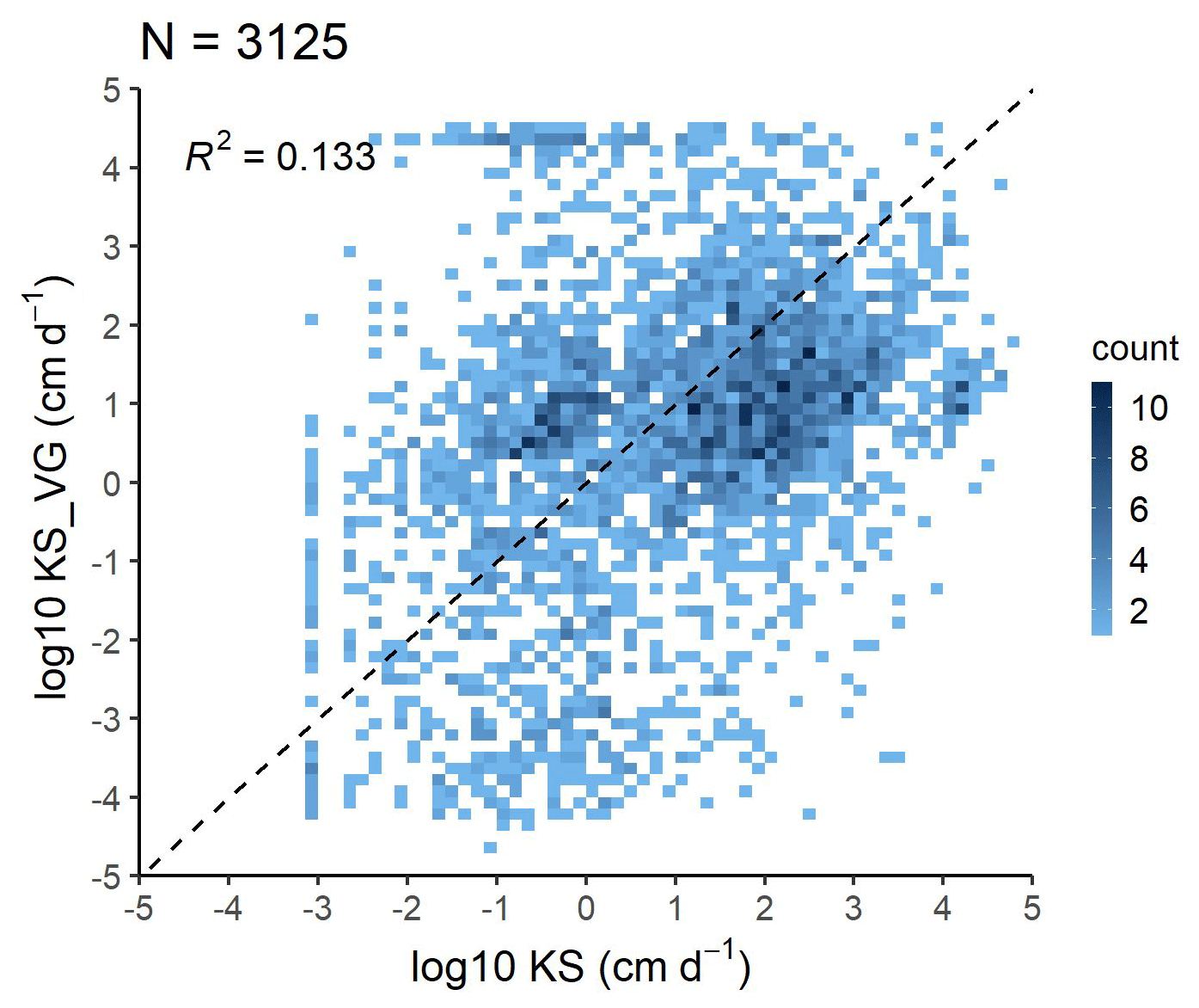
Figure 14 Scatterplot of measured saturated hydraulic conductivity (KS) versus saturated hydraulic conductivity computed from fitted VG parameters (KS_VG).

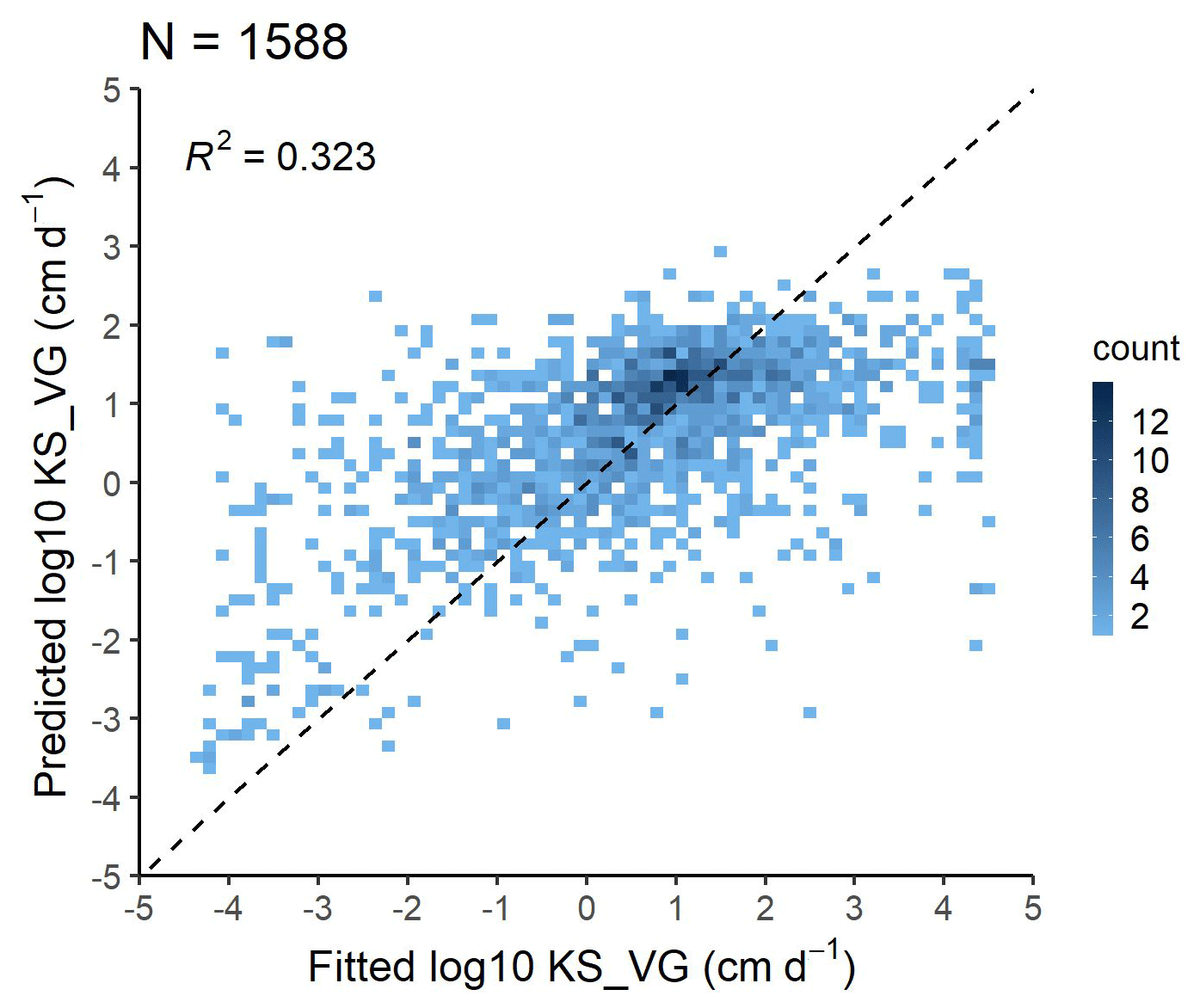
Figure 15 Scatterplot of saturated hydraulic conductivity computed from fitted and predicted VG parameters (KS_VG) analysed based on the VG test set of the EU-HYDI dataset. Count refers to the number of cases in each quadrangle.

Table 14 Prediction performance of saturated hydraulic conductivity (cm d⁻¹) computed by pedotransfer functions based on the VG test set of the EU-HYDI dataset. N refers to the number of samples, ME refers to the mean error, MAE refers to the mean absolute error, RMSE refers to the root mean squared error, NSE refers to the Nash–Sutcliffe efficiency, and R² refers to the coefficient of determination.

^* log10pred_KS_VG is the logarithmic-10-based saturated hydraulic conductivity computed based on VG parameters predicted from basic soil properties.

3.9 Phosphorus content of the topsoil

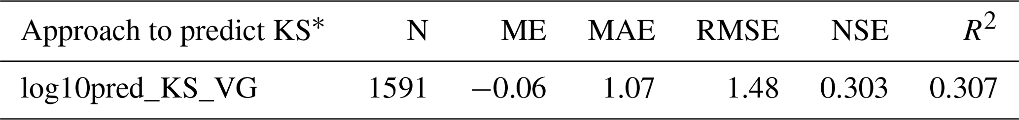
Figure 16 shows the European P map (Ballabio et al., 2019) clipped for the area of the Felső-Válicka study site (A) and the P map created with the mean statistics-based method using the local land use map (B) and the map of the hydrological response units (HRUs) defined in the SWAT+ model (C). The spatial pattern of the two phosphorus maps is similar, but the map created with our proposed method has a higher resolution and follows the polygons of the HRU map.

Figure 16 European topsoil P content map (Ballabio et al., 2019) (a), region-specific mean statistics-based P content map (b), and hydrological response units with indication of agricultural parcels with measured P values (c) in the Felső-Válicka case study.

Figure 17 shows the geometric mean P values of the HRUs by land use categories of the European soil P map and the region-specific mean statistics-based P map in the area of Felső-Válicka. Comparing the results of the geometric mean P values, we can see that the European topsoil P map, on average, has a higher P concentration, with no significant differences observed between the land use categories. Based on the region-specific LUCAS topsoil dataset, artificial land use areas (urban fabric and industrial, commercial and transport units), forests, and pastures are expected to have lower P concentration values. The mean statistics-based P map is more suitable in identifying differences resulting from local land use variations in the analysed case study. The P monitoring data measured on the 34 agricultural parcels, classified as arable land, show that the geometric mean of Olsen P in the area is 24 mg kg⁻¹, which is slightly higher than that predicted by the mean statistics-based method (19.78 mg kg⁻¹).

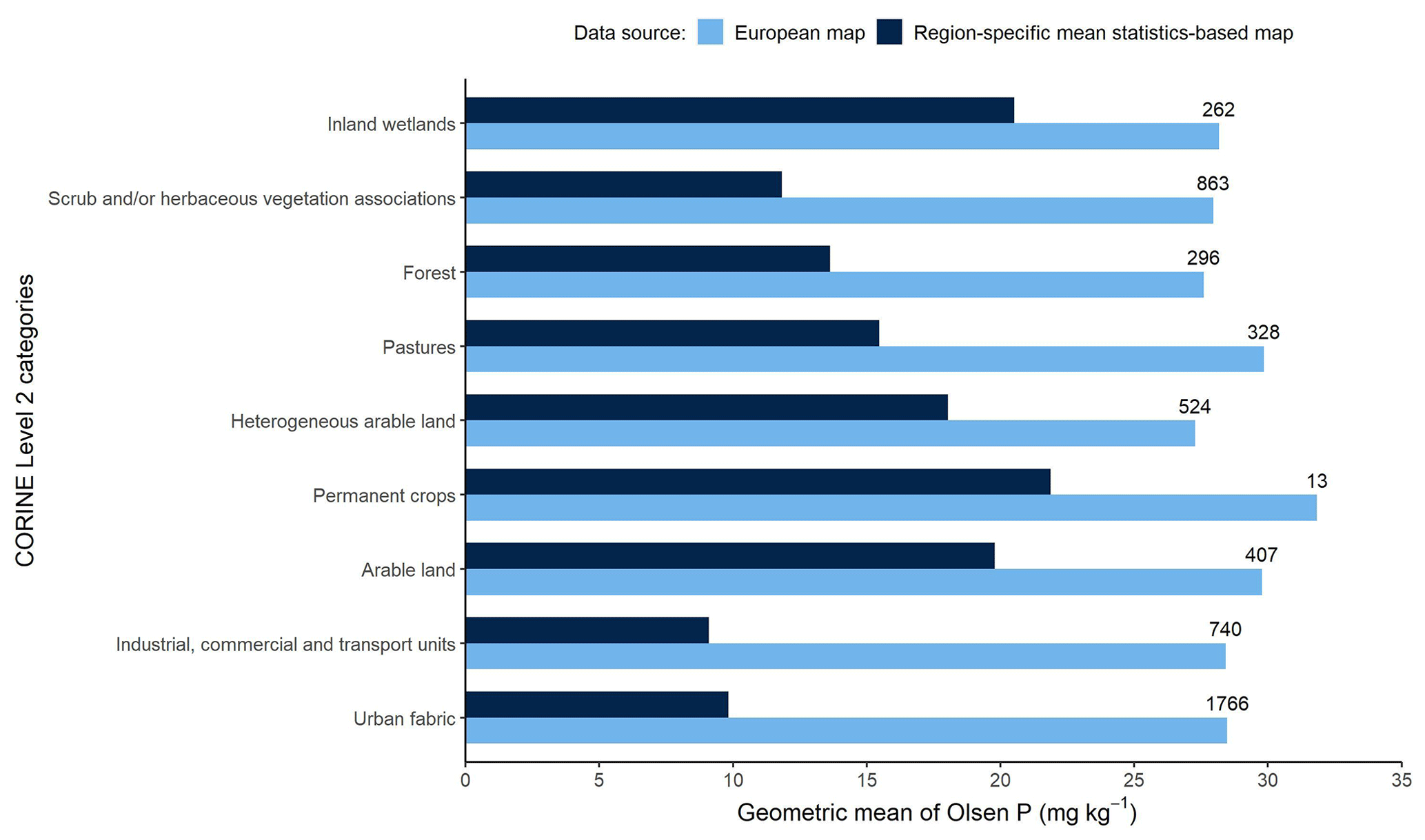
Figure 17 Geometric mean values of Olsen P across CORINE level-2 land cover categories in the Felső-Válicka case study for both the European topsoil P content map and the region-specific mean statistics-based P content map, with number of samples by category indicated.

Ballabio et al. (2019) found that land use was the most important predictor for computing the topsoil phosphorus content map for Europe. This underscores that a soil P content map derived based on a local, fine-resolution, field-boundary-based land use map can provide more accurate results than one based on continental land use maps.

For regional or local studies, it is more plausible to use a local land use map and to compute the geometric mean soil P values by land use categories based on the LUCAS topsoil dataset, which is relevant for the target area from a fertilization point of view. Where available, it is recommended that measured data be used to overwrite the geometric mean values, creating a multi-data source solution that reflects the spatial pattern of nutrient content within arable land areas. For continental-scale studies, the European topsoil P map (Ballabio et al., 2019) could be used.

3.10 Suggested workflow to derive soil input parameters

Based on the above results, we describe the most efficient workflow to retrieve the soil input parameters for European environmental modelling.

Initially, the data source of the most relevant soil basic properties, such as soil layering, rooting depth, organic carbon content, clay, silt, and sand content, must be selected. Local data can describe the spatial variability of soil properties the best. Even if only basic soil properties are available locally, this data source could be prioritized over the more inclusive continental or global datasets, i.e. those containing information on soil physical, chemical, and hydraulic properties because local datasets aim to capture the area-specific variability of soil properties as accurately as possible. If no local or national basic soil data are available with the resolution required to study a target environmental process, possible input sources for soil profile data or 3D soil datasets can be found in Table 1.

Different countries and institutions measure sand, silt, and clay content using different ISO protocols and methods by recognizing different cutoff limits and classification standards. It is important to check which particle size limits are required by the environmental model. As an example, in the widely used SWAT/SWAT+ model, the sand, silt, and clay content are assumed to be classified according to the USDA system, which defines the particle size limits of < 0.002 mm for clay, 0.002–0.05 mm for silt, and 0.05–2 mm for sand fraction. When conversions between different classifications are required to bring the local dataset to the appropriate format, it is advised that one apply the k-nearest-neighbour interpolation (formerly called: “similarity technique”), which results in less uncertainty, smaller bias, and shrinkage of the resulting texture range compared to the simpler log-linear interpolation (Nemes et al., 1999).

In other cases, such as for soil organic material, it is important to distinguish if soil organic carbon or soil organic matter is required by the model and which of the two is available from the data source. The following most frequently used equation describes the relationship between them:

$$\begin{array}{}\text{(21)}& \mathrm{OM}=\mathrm{OC}\cdot \mathrm{1.724},\end{array}$$

where OM is the organic matter content (mass %), and OC is the organic carbon content (mass %). The 1.724 conversion factor was defined by van Bemmelen (1890) but can vary between 1.4 and 2.5 depending on the method used to measure the organic carbon content, the composition of organic matter, the degree of decomposition, and the clay content (Minasny et al., 2020; Pribyl, 2010). Pribyl (2010) recommends using the value 2 as a general conversion factor if no specific value is available.

When specifying bulk density, it is important to clarify whether the dry or effective value is required. If no measured value of either one is available, the dry bulk density can be computed from the organic carbon content and particle size distribution. Further predictors, such as taxonomical information, soil structure, soil management parameters, and environmental covariates, are important as well (Hollis et al., 2012; Ramcharan et al., 2017) and can significantly improve the prediction performance. However, it is not always possible to apply PTFs including these variables to a data-scarce region.

If effective bulk density is required, it can be derived from the dry bulk density with the method of Wessolek et al. (2009):

• for soils with an organic carbon content higher than 0.58 mass %, the following is used:

  $$\begin{array}{}\text{(22)}& {\mathrm{BD}}_{\mathrm{eff}}={\mathrm{BD}}_{\mathrm{dry}}+\mathrm{0.009}\cdot \mathrm{clay},\end{array}$$

• for soils with an organic carbon content less than or equal to 0.58 mass %, the following is used:

  $$\begin{array}{}\text{(23)}& {\mathrm{BD}}_{\mathrm{eff}}={\mathrm{BD}}_{\mathrm{dry}}+\mathrm{0.005}\cdot \mathrm{clay}+\mathrm{0.001}\cdot \mathrm{silt},\end{array}$$

where BD_eff (g cm⁻³) is effective bulk density, BD_dry (g cm⁻³) is the dry bulk density, clay is clay content (< 0.002 mm, mass %), and silt is silt content (0.002–0.063 mm, mass %). It is important to note that Eq. (23) requires the silt content with a limit of 0.002–0.063 mm. It can be predicted from the clay (< 0.002 mm), silt (0.002–0.05 mm), and sand (0.05–2 mm) content with the TT.text.trans function of the soiltexture R package (Moeys, 2018). This method meets the accuracy required for computing BD_eff; however, for other applications, the transformation methods discussed by Nemes et al. (1999) should be considered.

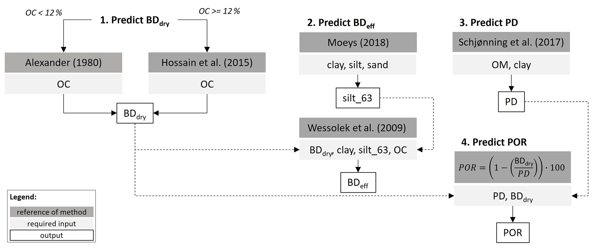
Figure 18 Prediction of soil physical properties. BD_dry refers to dry bulk density, clay refers to clay content (0–0.002 mm), silt refers to silt content (0.002–0.05 mm), sand refers to sand content (0.05–2 mm), silt_63 refers to silt content (0.002–0.063 mm), OC refers to organic carbon content, BD_eff refers to effective bulk density, PD refers to particle density, and POR refers to porosity.

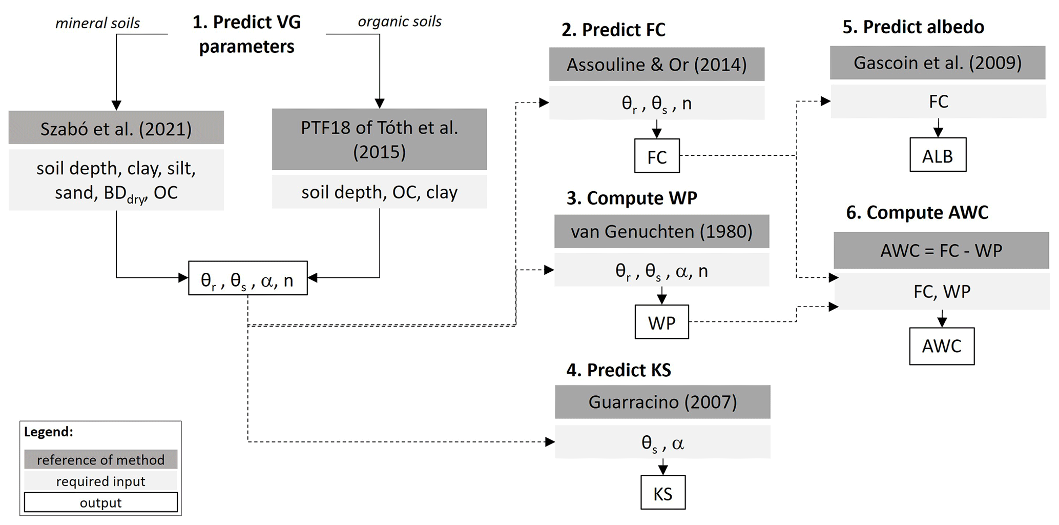
Figure 19 Prediction of soil hydraulic properties and moist soil albedo. Soil depth refers to the mean soil depth of the soil sample, clay refers to clay content (0–0.002 mm), silt refers to silt content (0.002–0.05 mm), sand refers to sand content (0.05–2 mm), BD_dry refers to dry bulk density, OC refers to organic carbon content, θ_r refers to residual water content, θ_s refers to saturated soil water content, α refers to the scale parameter, n refers to the shape parameter, FC refers to the water content at field capacity, WP refers to the water content at wilting point, KS refers to the saturated hydraulic conductivity, AWC refers to the available water capacity, and ALB refers to soil albedo.

The hydrologic soil groups (HSGs) are based on the infiltration characteristic of the soil and include four groups that have similar runoff potential. The groups are defined based on the saturated hydraulic conductivity, depth to the high water table, and depth to the water impermeable layer (Table 15). More details can be found in the documentation of the US Department of Agriculture Natural Resources Conservation Service (2009).

For modelling purposes, it is important to know whether tile drainage is present in the modelled area because tile drainage systems influence the soil infiltration rate and runoff potential. Derivation of HSGs requires local input data. If local datasets are not available and if SoilGrids 2017 (Hengl et al., 2017) was chosen as the source for the basic soil data, HSG can be retrieved from the global HYSOGs250m (Ross et al., 2018) database.

Table 15 Definition of soil hydrologic groups based on the US Department of Agriculture Natural Resources Conservation Service (2009). KS refers to saturated hydraulic conductivity (µm s⁻¹).

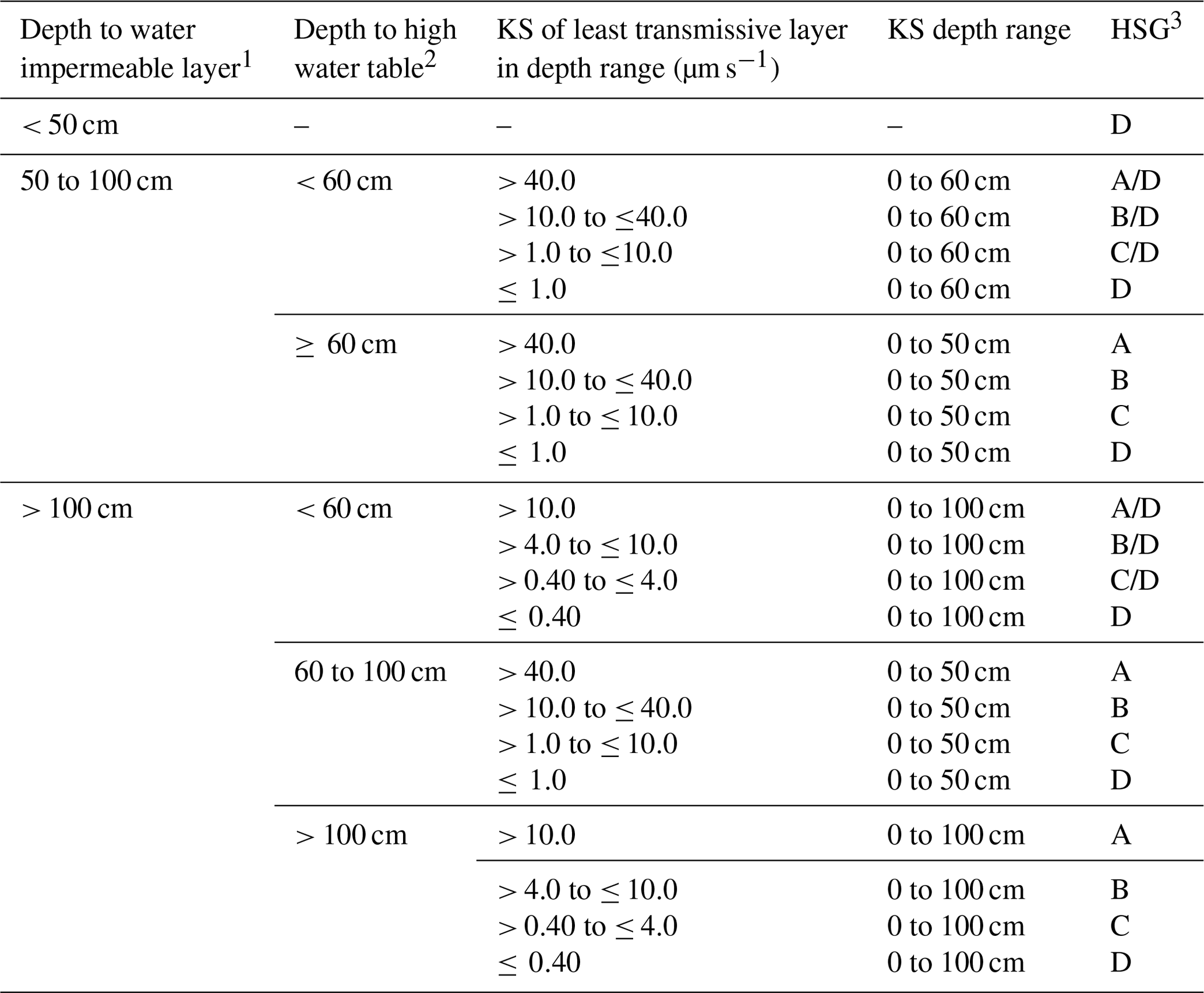
¹ An impermeable layer has a KS of less than 0.01 µm s⁻¹ (0.0014 in h⁻¹) or a component restriction of fragipan, duripan, petrocalcic, orstein, petrogypsic, cemented horizon, densic material, placic, paralithic bedrock, lithic bedrock, densic bedrock, or permafrost. ² High water table during any month during the year. ³ Dual HSG classes are applied only for wet soils (water table less than 60 cm or 24 in.). If these soils can be drained, a less restrictive HSG can be assigned, depending on the KS.

Figures 18–22 summarize the workflows to derive the soil physical, hydraulic, and chemical parameters covered in this study. The workflows highlight the target soil property, necessary input, and computation approach with a suggested order of computations. Indirect initialization of soil mineral N is recommended via proper management data and a model warm-up period. It is important to highlight that prediction approaches trained on local data are expected to be more accurate; therefore, those could replace the indicated methods where possible.

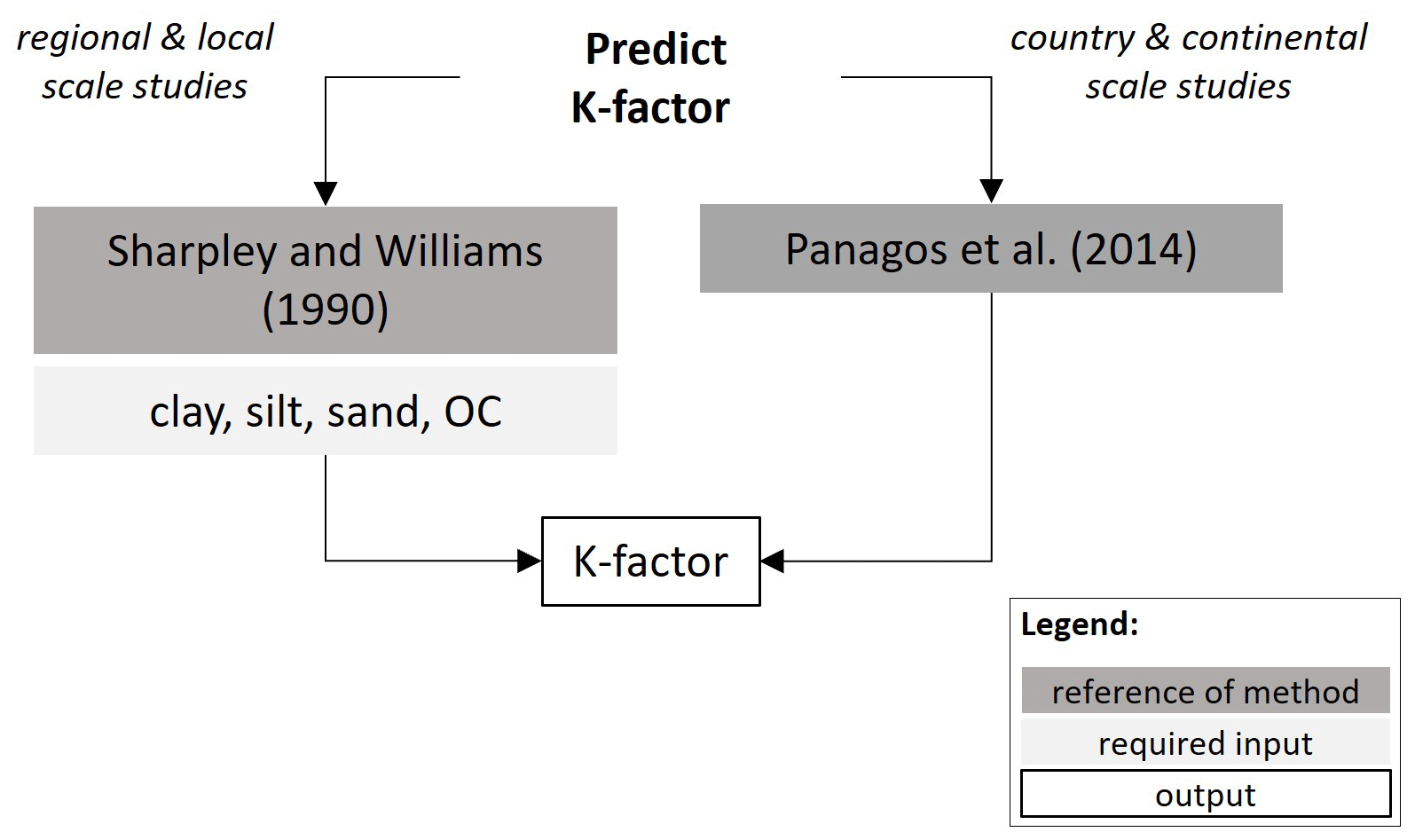
Figure 20 Prediction of soil erodibility factor (K factor). Clay refers to clay content (0–0.002 mm), silt refers to silt content (0.002–0.05 mm), sand refers to sand content (0.05–2 mm), and OC refers to organic carbon content.

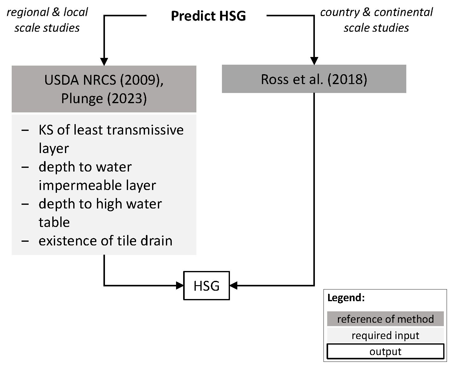
Figure 21 Prediction of hydraulic soil groups (HSGs). KS refers to saturated hydraulic conductivity.

4 Conclusions

This study presents particular techniques and resources for extracting region-specific soil characteristics from national and global databases. While these databases might contain segments of soil information, they often lack the comprehensive data required by various environmental models, such as the SWAT+ model. Through evaluation and recommendation of selected PTFs, as well as the provision of compiled R scripts for estimation solutions addressing soil data gaps, this study aims to streamline input data preparation procedures for soil physical, hydraulic, and chemical properties in environmental modelling.

Local data tend to retain finer soil details; hence, it is recommended that users prioritize the utilization of local (national) soil databases when they are deemed to be representative and reliable. Even if these databases only offer basic soil properties, they should take precedence over broader continental or global datasets. The study demonstrated that missing soil properties could be estimated effectively from a basic set of soil parameters using appropriate PTFs developed for specific pedo-climatic regions, ensuring consistency in computed properties.

We prepared a set of workflows to derive soil input parameters for usage in various modelling studies. In cases where this approach is not viable, we offer comprehensive guidance on alternative soil databases, outlining strategies to derive the absent soil properties effectively.

When using any available soil dataset, it is important to check the detailed description (metadata) of the dataset to avoid misinterpretation and errors in the models. Considerations such as consistent size limits for clay, silt, and sand content classification as per the model's requirements; the distinction between organic carbon and organic matter; the need for dry or moist bulk density; and similar details are vital. Understanding whether the model derives soil properties that already exist in the dataset is essential, aiding in selecting the most precise parameters for the model's application.

Figure 22 Prediction of Olsen phosphorus (P) content of the topsoil.

When retrieving or deriving missing soil input data, it is crucial to consider the following: (i) which dataset and prediction approaches can offer physically plausible soil input data and (ii) the uncertainty associated with the derived soil input data for their appropriate use in the environmental model. For computing physically consistent soil hydraulic property values, namely FC, WP, AWC, and KS, it is plausible to use parameters of a model that describe soil water retention across the entire matric-potential range. The parameters of the VG model have been widely employed to derive water retention at specific matric-potential values or KS; hence, they can be used to derive physically plausible soil hydraulic properties. The static definition of FC could be replaced with a dynamic one that considers a soil-specific matric potential at which the continuity of soil water is reduced or disrupted. For the computation of the drainage-dynamics-based AWC, the use of the VG model parameters is required for deriving both FC and WP. When computing FC, WP, AWC, and KS using the predicted VG parameters, we maintain the physical relationships among them, which is highly relevant in process-based modelling applications. Misuse of these parameters could lead to flawed model outcomes, impacting policy-making and agricultural management decisions.

It is important to note that soil parameter uncertainty encompasses not only the uncertainty of the PTF but also that stemming from the fitting of the VG model. The prediction uncertainty of soil properties varies significantly. It is essential to tailor its treatment based on the specificities of the target environmental model, particularly when it is utilized as an initial static value, in model calibration, or as a fixed input parameter.

The research emphasized the challenge of selecting suitable datasets and PTFs due to their abundance, providing quantitative performance metrics to aid potential environmental modellers. The workflows and findings presented in this study offer practical guidance for model setup and data pre-processing in various modelling endeavours across Europe, such as in hydrological simulations, assessments of soil health, land evaluation, crop modelling, and analysis of soil erosion risk, among others. The study's methodology can be applied for soil databases not only in Europe but also in other regions or global datasets, highlighting its potential for broader applicability in multiple modelling contexts worldwide. We encourage the wider scientific and modelling community to use and adopt our recommended workflows to derive soil input parameters, bridging gaps in the data for broader utilization in diverse modelling studies. The presented workflows could be further improved by using a multi-model approach and applying geostatistical methods. The open-source library is available (see “Code availability” section) for use and adoption to meet user-specific needs.