Best performances of visible–near-infrared models in soils with little carbonate – a field study in Switzerland

Conventional laboratory analysis of soil properties is often expensive and requires much time if various soil properties are to be measured. Visual and near-infrared (vis–NIR) spectroscopy offers a complementary and cost-efficient way to gain a wide variety of soil information at high spatial and temporal resolutions. Yet, applying vis–NIR spectroscopy requires confidence in the prediction accuracy of the infrared models. In this study, we used soil data from six agricultural fields in eastern Switzerland and calibrated (i) field-specific (local) models and (ii) general models (combining all fields) for soil organic carbon (SOC), permanganate oxidizable carbon (POXC), total nitrogen (N), total carbon (C) and pH using partial least-squares regression. The 30 local models showed a ratio of performance to deviation (RPD) between 1.14 and 5.27, and the root mean square errors (RMSE) were between 1.07 and 2.43 g kg⁻¹ for SOC, between 0.03 and 0.07 g kg⁻¹ for POXC, between 0.09 and 0.14 g kg⁻¹ for total N, between 1.29 and 2.63 g kg⁻¹ for total C, and between 0.04 and 0.19 for pH. Two fields with high carbonate content and poor correlation between the target properties were responsible for six local models with a low performance (RPD < 2). Analysis of variable importance in projection, as well as of correlations between spectral variables and target soil properties, confirmed that high carbonate content masked absorption features for SOC. Field sites with low carbonate content can be combined with general models with only a limited loss in prediction accuracy compared to the field-specific models. On the other hand, for fields with high carbonate contents, the prediction accuracy substantially decreased in general models. Whether the combination of soils with high carbonate contents in one prediction model leads to satisfying prediction accuracies needs further investigation.

1 Introduction

The application of spectroscopy in the visible and near-infrared (vis–NIR) range is increasing in soil science and related disciplines, with the main objective being to gain information on the soil properties of more samples at lower costs than with conventional laboratory methods. With a larger sample size, the spatial or temporal resolution can be increased, which allows conclusions about the within-field or within-farm variability but might potentially also increase the statistical power in agricultural experiments (Greenberg et al., 2022). Despite its tendency to be less accurate compared to mid-infrared (MIR) spectroscopy, vis–NIR spectroscopy is widely applied because of less sample preparation, lower costs and generally easier portability (Soriano-Disla et al., 2014).

On-site vis–NIR measurements are therefore feasible, but laboratory measurements with dried and sieved soil samples have so far shown higher accuracy (Allory et al., 2019; Hutengs et al., 2019). In particular, soil properties related to soil organic matter can be estimated appropriately by laboratory vis–NIR spectroscopy (Angelopoulou et al., 2020). In most cases, the focus is to provide soil information over large areas (e.g., soil maps) where a high sample number is present and only a moderate prediction accuracy is needed. Hence, large-scale spectral libraries have been developed to further reduce the need for wet chemistry data. Due to the high complexity within spectral libraries, the application of a general model to a local context leads to high prediction errors. Recent research shows that the localization of these infrared models substantially improves the predictive performance in a local context, for example by spiking (Brown, 2007; Li et al., 2020; Ng et al., 2022; Seidel et al., 2019; Wetterlind and Stenberg, 2010; Zhao et al., 2021), memory-based learning (Ramirez-Lopez et al., 2013), resampling algorithms (Lobsey et al., 2017) or deep learning (Shen et al., 2022). However, for analyzing small-scale variability (field or farm level), a local model is often still the best choice because of its low prediction errors. Theoretically, developing local models is supported by the finding that, in the vis–NIR range, spectral features that influence specific soil properties vary strongly between different datasets, which makes highly heterogenous large datasets prone to insufficient model performance (Angelopoulou et al., 2020; Grunwald et al., 2018). The development of local spectral models has the main purpose of coping with a large sample size at the local scale, but such local models have no utility beyond the analysis of the specific local dataset.

Spectral vis–NIR models developed from local datasets showed a very high variability in model performance, ranging from excellent models (Breure et al., 2022; Seidel et al., 2019) to those with relatively poor model performance (Camargo et al., 2022; Kuang and Mouazen, 2011). The reasons for these different performances of local models are understudied and remain unclear. Among many different possible modeling approaches, including support vector machine regression, artificial neural networks, cubist and random forest, partial least-squares regression (PLSR) is the most frequently used model type to build spectral models with small datasets (Alomar et al., 2021; Zhao et al., 2021).

The number of samples is crucial for local models , often, only a limited number of samples with reference laboratory data are available. Kuang and Mouazen (2012) showed that local models improve with an increasing number of calibration samples and that a sample size of at least 50 provides accurate prediction models. Some studies thus combined multiple target sites and developed a general model by combining all the local datasets to reach a larger sample size and potentially better model performance (Kuang and Mouazen, 2011; Singh et al., 2022). In these studies, the general model showed an intermediate performance, and the general prediction error was between the best- and the poorest-performing local model. However, these studies only calculated the overall prediction error of the general model; therefore, it is not clear if the prediction for target sites with poorly performing local models could be improved by applying a general model.

For vis–NIR spectroscopy application at local scales, it is therefore very difficult to estimate the measurement accuracy for the predicted samples beforehand. This uncertainty is probably the main reason that hampers the application of vis–NIR spectroscopy because researchers prefer to rely on conventional lab measurements with a smaller sample size (and smaller spatial resolution) where the measurement accuracy is known before sampling and measurements are conducted. Applying spectroscopy at the field or farm scale thus bears the risk that the measurement accuracy (RMSE) may be beyond the tolerable threshold, which might then bring a whole project into question. Thus, in this paper, we analyze the performance of field-specific (local) spectral models of a field experiment conducted in six fields in eastern Switzerland and that of a general model combining the data from all six fields to ascertain their influencing factors. We ask the following questions:

1. To what extent do the prediction errors of local spectral models differ from the lab measurement error?

2. Does a general model that includes several target sites improve the prediction on a target site with a poor local-model performance?

3. How do field and soil characteristics (e.g., field size, soil texture, carbonate content, correlations of soil properties) of the target site relate to the performance of spectral models?

By answering these questions, we want to provide insights into the estimations of prediction accuracies for vis–NIR studies at the local scale, with the objective of supporting decision-making during the development of a sampling design and the planning of laboratory reference measurements for subsequent calibration modeling.

2 Methods

2.1 Datasets from a cover-cropping experiment at six field sites

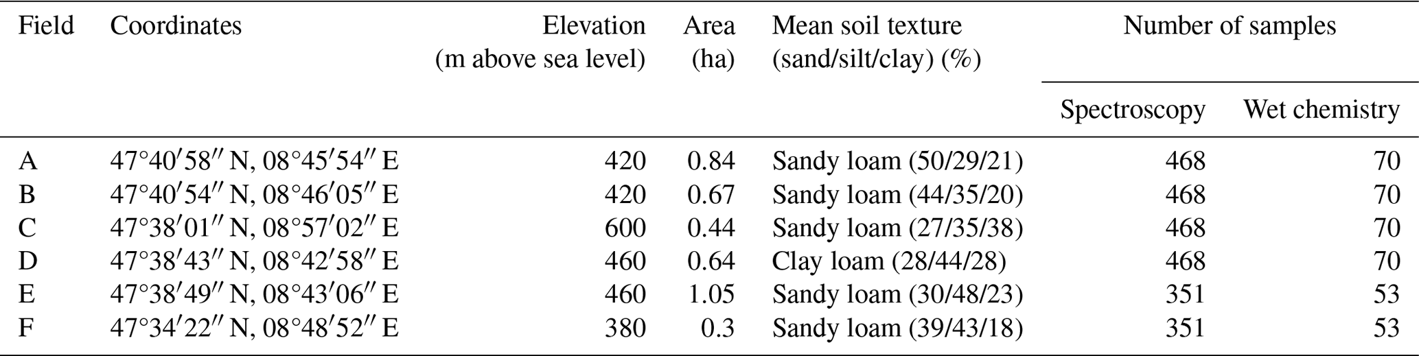
We used datasets from six fields (A, B, C, D, E, F) of a cover-cropping experiment in the Canton of Thurgau, eastern Switzerland (paper in preparation). The six fields were up to 13 km apart from one another, and the soil type for all of them was Eutric Cambisol that had developed on base moraine (Table 1). The aim of the study was to compare the influence of two different cover-cropping regimes on short-term soil organic matter cycling. Each field had 39 differential-GPS (dGPS)-referenced sampling points in an unaligned sampling design. At each dGPS-referenced point, soil was sampled three to four times at three depths (0–5, 5–10 and 10–20 cm) during one long cover-cropping period (August 2019 to May 2020). Fields A, B, C and D had four sampling times, resulting in 468 samples per field. Fields E and F had three sampling times, resulting in 351 samples per field. All samples were dried at 40 °C to a constant weight (around 72 h) and then gently crushed and sieved to 2 mm. For the total sample size of 2574 samples, soil properties were estimated using vis–NIR soil spectroscopy, whereas 386 samples were analyzed conventionally by wet chemistry for subsequent calibration modeling. These 386 samples for laboratory analysis were selected for each field separately using the Kennard–Stones algorithm (Kennard and Stone, 1969) to ensure coverage of the whole spectral variability. Thereby, the Kennard–Stones algorithm was run with two to seven principal components, and the number of principal components was chosen such that it covered at least 99 % of the spectral variance and provided a reference sample selection that represented well the different sampling times, soil depths and spatial distributions. The laboratory analysis comprised soil organic C (SOC), total C, total N, permanganate oxidizable C (POXC) (also called active C) and pH.

Table 1 Description of the datasets of the six different fields A to F. All fields were classified as Eutric Cambisol developed on base moraine. Soil texture was measured with the improved integral suspension pressure method (ISP+).

2.2 Chemical soil analyses and its accuracy

Total C and N concentrations were measured on a ground aliquot by dry combustion (vario MICRO tube, Elementar, Germany). Inorganic C was analyzed for each sample in triplicates through the dissolution of carbonate in a Scheibler apparatus with 10 % HCl solution and the measurement of the evolved CO₂ volume. SOC was then calculated as the difference between total C and the mean of the three measurements for inorganic C. POXC was measured according to the Protocol of Weil et al. (2003), with the adaption of Lucas and Weil (2012). In brief, 2.0 mL of 0.2 M KMnO₄ was added to 2.5 g of soil, and after a reaction time of 10 min, the absorption of the liquid was measured at 550 nm with a spectrophotometer (UV-1800, Shimadzu Corporation, Japan). The measurement of pH was done in a 0.01 M CaCl₂ solution.

To estimate the lab measurement error, we took three samples per field (in total 18) where we conducted the measurements for total C, total N, POXC and pH in triplicates to calculate a standard deviation. We estimated the lab measurement error for SOC (σ_SOC) according to Eq. (1):

$$\begin{array}{}\text{(1)}& {\mathit{\sigma }}_{\mathrm{SOC}}=\sqrt{{\mathit{\sigma }}_{\mathrm{Total}\mathrm{C}}^{\mathrm{2}}+{\mathit{\sigma }}_{\mathrm{Inorganic}\mathrm{C}}^{\mathrm{2}}},\end{array}$$

where σ_Total  C is the standard deviation of the total C measurement, and σ_{Inorganic  C} is the standard error of the inorganic C measurement because inorganic C measurements were done for all samples in triplicates. The measurement errors of all 18 triplicates were then averaged to obtain the overall lab measurement error for a soil property.

To characterize the spatial variability of soil texture in the field, we measured grain size for 20 samples per field (every second sampling point in 10–20 cm soil depth). Organic matter in the samples was oxidized with hydrogen peroxide (H₂O₂), and then grain size was measured with laser-diffraction analysis (LDA) after dispersion of the sample (22 mM sodium carbonate and 18 mM sodium hexaphosphate) using a Mastersizer 2000 (Malvern Panalytical, UK). Since the LDA underestimates the clay content compared to the standard grain size methods (Taubner et al., 2009), we measured one composite sample per field with the improved integral suspension pressure method (ISP+; Durner and Iden, 2021) on a PARIO Plus Soil Particle Analyzer (METER Group, Germany and USA). We rescaled the mean sand, silt and clay content of the LDA data to the mean of the IPS+ method while keeping the coefficient of variation constant (see Table S3 in the Supplement).

2.3 Spectral measurement and pre-processing of spectra

All samples were measured with a vis–NIR spectrometer (ASD FieldSpec 4 Hi-Res, Malvern Panalytical, USA) with a sampling interval of 1.4 nm from 350 to 1000 nm and 1.1 nm from 1000 to 2500 nm. The device then provides a reflectance spectrum with a resolution of 1 nm and 2151 wavelengths. Measurements were done with a contact probe, containing an internal halogen bulb, which was in a fixed position, and soil samples, placed in a petri dish of 1.5 cm height and 3 cm diameter, were lifted with a laboratory scissor jack until coming into close contact with the probe to ensure a stable measurement position. For each sample, five petri dishes were filled to provide five replicate spectra per sample. Each of these five replicates consisted of 30 internal repetitive scans that were automatically averaged by the device's internal RS3 software. Between samples, the contact probe was carefully cleaned with water and ethanol. After the five replicates of a sample, the calibration of the spectrometer was checked with a 100 % reflectance white reference panel (Spectralon, 12 × 12 cm, Labsphere, USA). The infrared data of each sample were kept in two versions, once as reflectance spectra, as provided by the spectrometer, and once as absorbance spectra using the log($\mathrm{1}/$ reflectance) transformation. Several pre-processing options and their combinations were tested on both the reflectance and the absorbance spectra: (a) resampling of the spectra in an interval from 1 to 6 nm, (b) cutting of the beginning (350–400 nm) or the end (2450–2500 nm) of the spectra, (c) first- or second-order derivative, (d) Savitzky–Golay (SG) smoothing in a third-order polynomial with window sizes ranging from 5 to 51, (e) gap segment derivative (GSD) with window widths between 5 and 51 and segment sizes between 1 and 21, (f) standard normal variate (SNV) combined with GSD, and (g) SG smoothing combined with multiplicative scatter correction (MSC). All applied pre-processing techniques are frequently used in soil spectroscopy and are well described in Ellinger et al. (2019). The pre-processing techniques from (a) to (g) led to around 100 meaningful combinations that were tested in model building, and the final pre-processing option was selected based on the smallest RMSE.

2.4 Development and evaluation of field-specific local models

We used for all 30 local models (6 fields × 5 properties) a PLSR modeling approach (Wold et al., 1983). Model performance was assessed using the statistics of the hold-out folds of each five-times-repeated five-fold cross-validation because it was evaluated as a robust method for smaller datasets (Kuhn and Johnson, 2013; Molinaro et al., 2005). To avoid model overfitting, we set the maximum of latent variables in the PLSR model to 12. For each number of latent variables (1, 2, …, 12) the dataset was randomly split five times into five folds, of which four were used for model training, and the remaining fold was held out and used for model validation. The RMSE (Eq. 2) of the hold-out samples was averaged among the five repeats, resulting in a cross-validated RMSE per number of latent variables. The final number of latent variables was then chosen according to the “1-standard-error rule”, which means that, instead of directly choosing the number of latent variables with the smallest mean RMSE, the most parsimonious (fewer latent variables) model within 1 standard error of the mean RMSE of the optimal model was selected (Hastie et al., 2017). The 1-standard-error rule was also applied during optimization of pre-processing to avoid model overfitting. The final model was trained using all training data with an optimized number of latent variables.

A proper validation of a spectral model is very crucial and is particularly important in this study where soil was repeatedly sampled at different depths at the same GPS point. To analyze the correlation among the samples and define a grouping factor for the cross-validation, we calculated the mean Euclidean distance between all samples and compared it with the mean distance (1) between samples at the same GPS point but different depths, (2) between samples at the same point and depth but different sampling times, and (3) between samples at the same point but different depth and sampling times (Fig. S1 in the Supplement). Thereby, we observed that the soil samples from the three different soil depths sampled at the same GPS point at the same sampling time had a substantially lower mean Euclidean distance compared to the overall mean. Consequently, we grouped the samples from the same GPS point at the same sampling time and kept them in the same fold to avoid a too-optimistic model evaluation during cross-validation.

Since we used a cross-validation approach at the field scale, all models showed a very small bias (see Table 2). We therefore do not discuss the bias in this paper and focus on R², RMSE and RPD (Eq. 3) for the evaluation and comparison of different models. RMSE was calculated according to Eq. (2), where ${\widehat{y}}_i$ is the prediction of the spectral model for sample i, and y_i is the actual measured value for the same sample in the laboratory.

$$\begin{array}{}\text{(2)}& \mathrm{RMSE}=\sqrt{{\displaystyle \frac{\mathrm{1}}{n}}{\sum }_{i=\mathrm{1}}^n{\left(y_i-{\widehat{y}}_i\right)}^{\mathrm{2}}}\end{array}$$

RPD compares the RMSE with the standard deviation (SD, Eq. 3) of the data:

$$\begin{array}{}\text{(3)}& \mathrm{RPD}={\displaystyle \frac{\mathrm{SD}}{\mathrm{RMSE}}}.\end{array}$$

For all model performance parameters (R², RMSE and RPD) of the cross-validation, we calculated the uncertainty with the standard deviation of the prediction of the hold-out folds across the five repetitions.

Table 2 Description of applied pre-processing and model performance of the final chosen models using a partial least-squares regression. The local models (fields A to F) were evaluated with five-times-repeated 5-fold cross-validation, and the general models (all) were evaluated with five-times-repeated 10-fold cross-validation. Model metrics of cross-validation are indicated as mean with the standard deviation across the repeats in brackets. RMSE refers to root mean square error, RPD refers to ratio of performance to deviation, Refl. refers to reflectance, Abs. refers to absorbance, SG refers to Savitzky–Golay filter (m refers to order of derivative, w refers to window width), SNV refers to standard normal variate, GSD refers to gap segment derivative (m refers to derivative, w refers to window width, s refers to segment size), and MSC refers to multiplicative scatter correction.

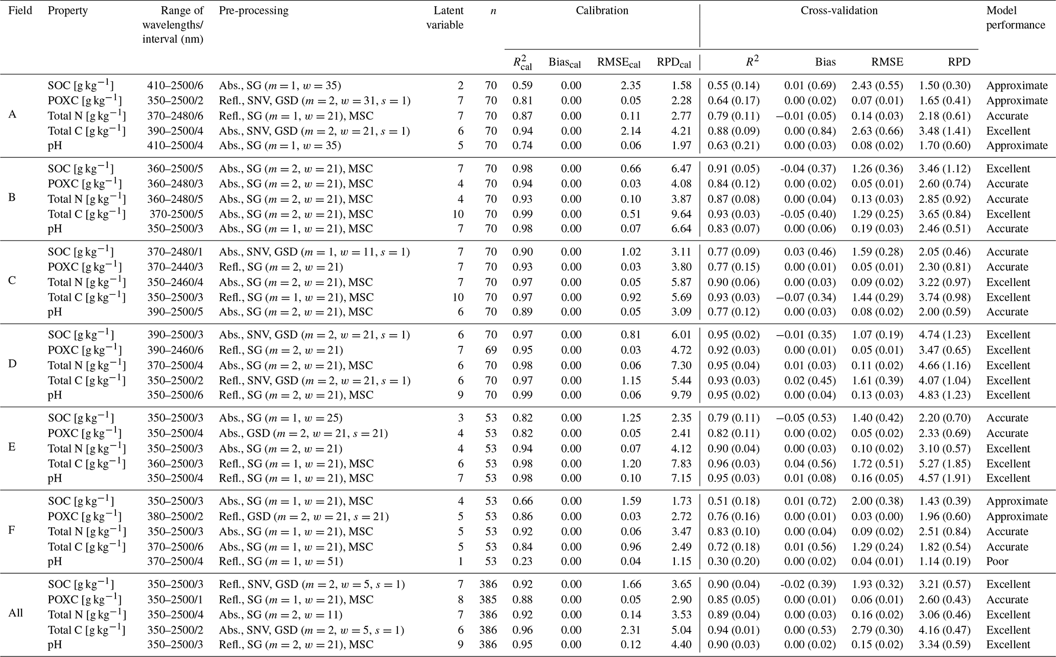
To classify the model performance, we combined the RPD-based classifications of Chang et al. (2001) and Zhang et al. (2018). We considered spectral models with RPD < 1.4 to be poor, models with RPD between 1.4 and 2 to be approximate, models with RPD between 2 and 3 to be accurate, and models with RPD > 3 to be excellent. Even though in spectroscopy projects relating to local extent the RMSE is the most important model performance parameter, RPD is the best parameter to compare models of different scales. Model metrics (R², RMSE and RPD) mentioned in the text are based on the cross-validation, and metrics for the model calibration in Table 2 are specifically labeled as $R_{\mathrm{cal}}^{\mathrm{2}}$, RMSE_cal and RPD_cal.

2.5 Development and evaluation of general models

In addition to the field-specific local models, we built general models for the five soil properties that included all reference samples (n=386) of the six fields. Even though for this sample size an independent test set would be more suitable than a cross-validation approach, we evaluated the model performance using the hold-out samples in the five-times-repeated 10-fold cross-validation, keeping, as for the local models, samples from the same GPS point and the same sampling time in the same fold. The first reason for not using an independent validation set is that the modeling approach of the general model should be similar to the one of the local models to make them comparable. The second reason is that a representative split of the dataset into a calibration and a validation set according to the spectral variability would not result in an equal number of samples per field in the validation set. Conversely, if we selected an equal sample size per field for the validation set, we would not have been able to cover the entire spectral variability. Evaluating the general models with hold-out samples of the cross-validation allowed us to calculate not only the RMSE over all samples but also the RMSE for the samples of each field individually. These field-specific RMSE values of the general model could then be compared with the RMSE values of the local models. Since the only purpose of the general models was to increase modeling efficiency for a specific combined dataset, we did not group the samples according to fields during cross-validation because the same share of samples from the same field would also be in the prediction dataset. For the general models, we cannot indicate uncertainties at a field-specific level since the folds did not always contain the same number of samples per field.

2.6 Model interpretation

To interpret spectral models, it is crucial to find relevant spectral features that are consistently important for a certain soil property. To identify the most important wavelength ranges in the final chosen models, we used the variable importance in projection (VIP) method first published by Wold et al. (1993) and evaluated by Chong and Jun (2005). The VIP method can deal with multicollinearity and is therefore suitable for the interpretation of spectral models as it was, for example, applied by Baumann et al. (2021). Wavelengths that have an above-average impact on the model have a VIP score above 1. We classified spectral ranges in groups of VIP scores between 1 and 1.5, 1.5 and 2, and above 2.

2.7 Assessment of site characteristics influencing model performance

To understand the reasons for the varying performance of the 35 developed spectral models, we studied the influence of various site characteristics on the models. To do so, we correlated the model performance parameters (R², RPD and RMSE) with field size, soil texture and carbonate content and with the correlation coefficients between SOC and total N in the dataset. With six local datasets as independent variables it is hardly possible to apply statistical tests that could potentially reject a null hypothesis. Therefore, we relied on the interpretation of graphs and Pearson's moment correlation coefficients between soil properties and RMSE. Since the RMSE values are estimates with uncertainties (standard deviations; see Sect. 2.4), we used a Monte Carlo simulation and reported the mean and standard deviation of the correlation coefficients after 1000 iterations. For the identified site characteristics that showed the strongest trends in terms of model performance (carbonate content, correlation coefficient between SOC and N and variability in clay content), we looked for possible explanations in the spectral features. Thereby, we relied on the VIP analysis of the trained models, on the correlation coefficients between soil properties with spectral variables and on the correlation matrices between target variables.

2.8 Data organization

All analyses were performed in R version 4.0.3 (R Core Team, 2020). The spectral datasets were analyzed using the R package simplerspec version 0.2.0 (Baumann, 2019) in combination with the packages prospectr version 0.2.1 (Stevens and Ramirez-Lopez, 2020) and caret version 6.0–86 (Kuhn, 2020).

3 Results

3.1 Description of the datasets

A comparison of the data distribution between the six different fields can be seen in Fig. 1, and the corresponding statistics can be seen in Table S1 in the Supplement. The means for SOC, total N and POXC differed between the six fields, but the distribution was relatively similar for these three soil properties. The density functions for total C and pH were highly influenced by the spatial distribution of carbonate in the soil: fields B, D and E contain samples with and without carbonate, resulting in a broad distribution for both total C and pH. All soil samples of fields A and C contained carbonate in varying concentrations, resulting in a broad distribution for total C but a narrow distribution for pH. Field F showed high and only slightly varying carbonate content and therefore a very narrow distribution for total C and pH. Field C had highest mean clay content, and field A had the highest mean sand content, whereas field F showed the highest variability in soil texture.

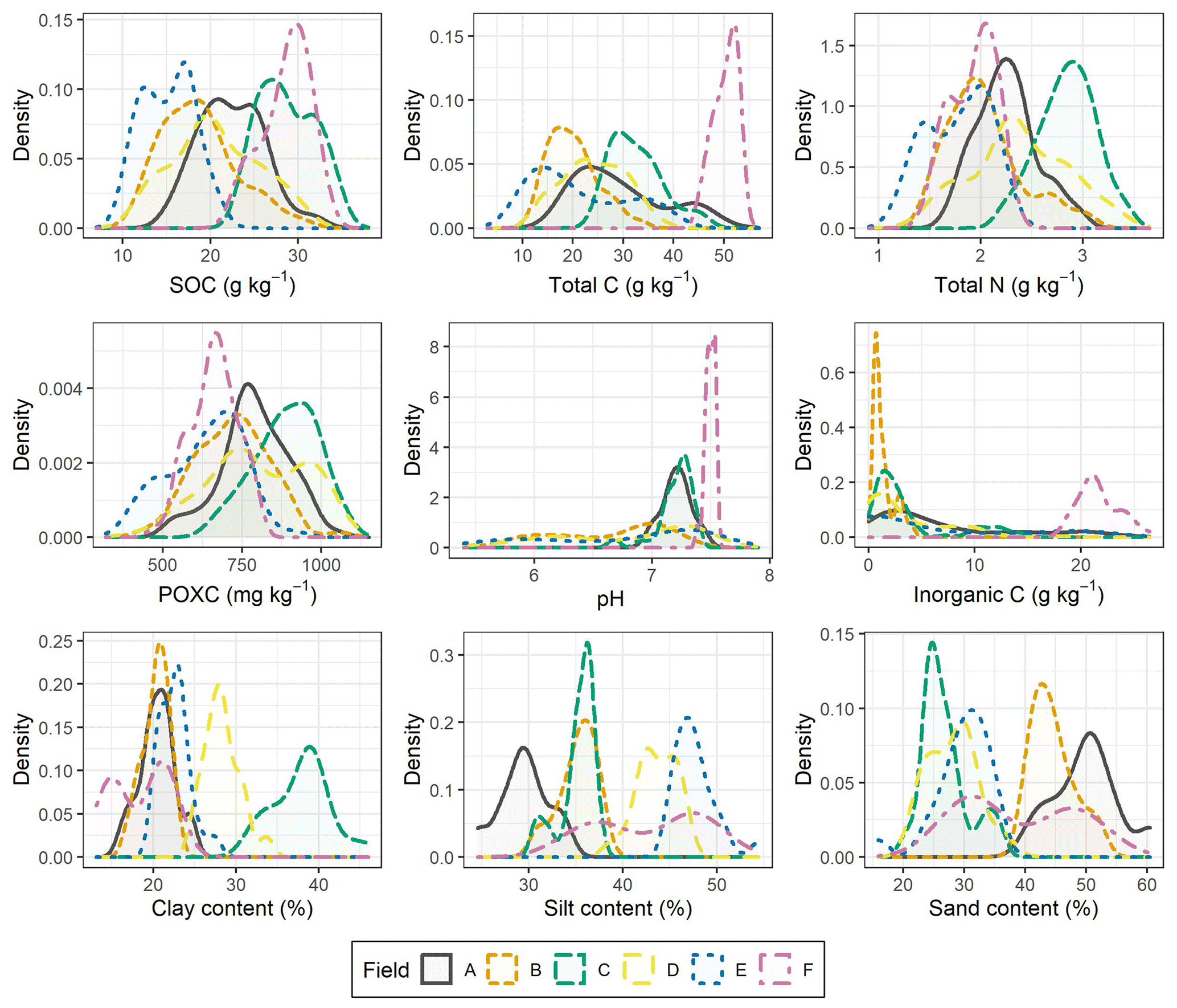
Figure 1 Density plots of the reference samples for the five target properties (SOC, total C, total N, POXC and pH) and inorganic C. Fields A to D each contained 70 samples, and fields E and F each contained 53 samples. Soil texture was analyzed in 20 samples per field.

3.2 Performance of spectral models

Based on RPD, 13 out of 30 local models showed an excellent performance (RPD > 3), 11 models an accurate performance (RPD > 2), 5 models an approximate performance (RPD > 1.4), and 1 model a poor performance (RPD > 1.4; Table 2). The six models without accurate performance were SOC, POXC and pH in fields A and F.

However, the RMSE values of the local models for pH of fields A (0.08 ± 0.02; mean ± standard deviation) and F (0.04 ± 0.01) were similar to or smaller than the RMSE of the other three local models (between 0.08 ± 0.02 and 0.19 ± 0.03) whose performances were classified as accurate. Differently, the local models for SOC in fields A and F with only approximate performance showed a higher RMSE (2.43 ± 0.55 and 2.00 ± 0.38 g kg⁻¹) than the other accurately performing local models for SOC (between 1.07 ± 0.19 and 1.59 ± 0.28 g kg⁻¹). The five general models all showed an accurate to excellent performance, with RPD values ranging from 2.60 ± 0.43 to 4.16 ± 0.47.

3.3 Influence of pre-processing on spectral variability

For all 35 models, pre-processing improved the models compared to the raw spectra (see an example of pre-processing optimization for total C in Table S2 in the Supplement). Although pre-processing was necessary for all models, we highlight that several pre-processing options performed similarly well within 1 standard deviation, and the differences in RMSE were often relatively small (see Table S2 in the Supplement). Figure S2 in the Supplement gives an overview of the best-performing pre-processing techniques. Most times, the first- or second-order derivatives improved the models substantially. Most models performed best when the spectra were reduced to every third wavelength and when models based on absorbance were a bit more frequently used than models based on reflectance. The combined application of SG filter and MSC was the most successful pre-processing, while a single SG filter, GSD and SNV in combination with GSD were of minor importance. Cutting of the beginning (350–400) or end of the spectra (2450–2500) sometimes improved the model performance, but since most pre-processing steps reduce the beginning and end of the spectra, it was not possible to evaluate the cutting. Similarly, it was not possible to evaluate the window width chosen in the SG filter because there is an interference with the resampling interval. A detailed list of the selected pre-processing options of the final models and the corresponding metrics for model performance can be found in Table 2.

The sensitivity of model performance to pre-processing can be visualized with the biplots of principal component analysis (PCA). Figure 2 shows the first three biplots of the raw spectra and the spectra that were pre-processed according to the general models of the five soil properties. The raw spectra had a very high share of the explained variance (96.8 %) for the first principal component but hardly any groups according to fields could be observed with the first two principal components. All pre-processing options used for the general models decreased the explained variance for the first principal component (32.5 % to 39.6 %), and a grouping according to fields could already be seen in the biplot of the first two principal components. Thereby, in particular, field F (with the highest carbonate content) and field C (with the highest clay content) often showed clear groups. Nevertheless, in the pre-processing for pH, field E (with the highest pH variability) shows a clear group in the first biplot, and the pH variability is well represented with the first PC.

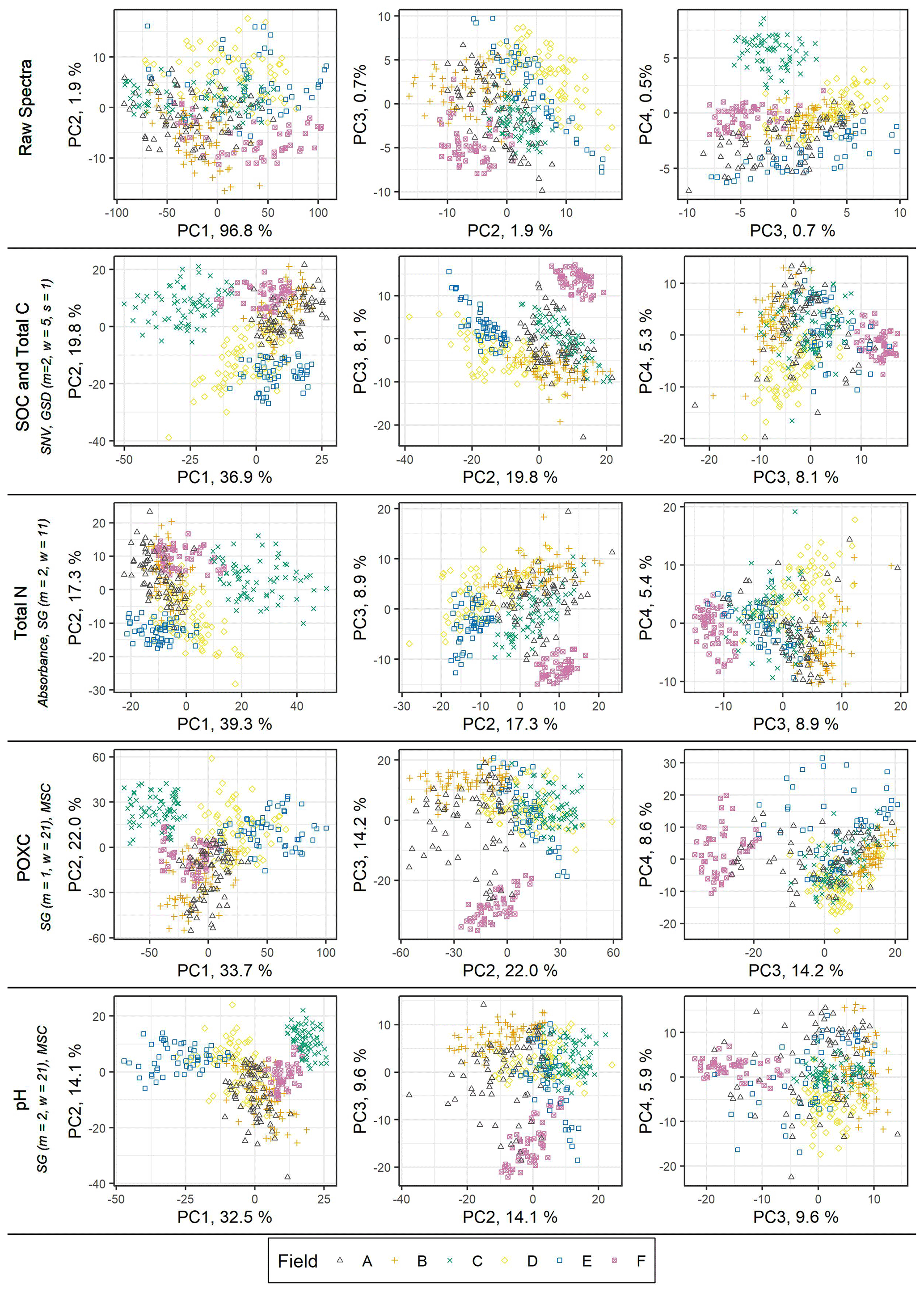
Figure 2 Biplots of principal component analysis with the first four principal components for the raw spectra and the pre-processed spectra according to the properties SOC, total C, total N, POXC and pH. The pre-processing is indicated in the figure, and, except for total N, it was conducted on reflectance spectra (SG refers to Savitzky–Golay filter (m refers to order of derivative, w refers to window width), SNV refers to standard normal variate, GSD refers to gap segment derivative (m refers to derivative, w refers to window width, s refers to segment size), and MSC refers to multiplicative scatter correction).

3.4 Comparison of general models with local models and lab measurement error

The overall cross-validated model metrics of the general model (filled black circle in Fig. 3) indicated a good performance over all fields for all soil properties, but the field-specific model evaluation showed distinct differences among fields. The field-specific R² of the general models of fields B, C, D and E was similar to the R² of the local model for SOC, total C, total N and POXC (only a slight slope in Fig. 3). For pH, only fields C, D and E showed similar R² in the local and general models, while fields A, B and F showed clearly higher R² in the local model. On the other hand, field F had clearly lower R² in the general model than in the local model for all soil properties except POXC. For field A, R² was similar between the local and the general models for SOC, total C and POXC but clearly lower for total N and pH in the general model.

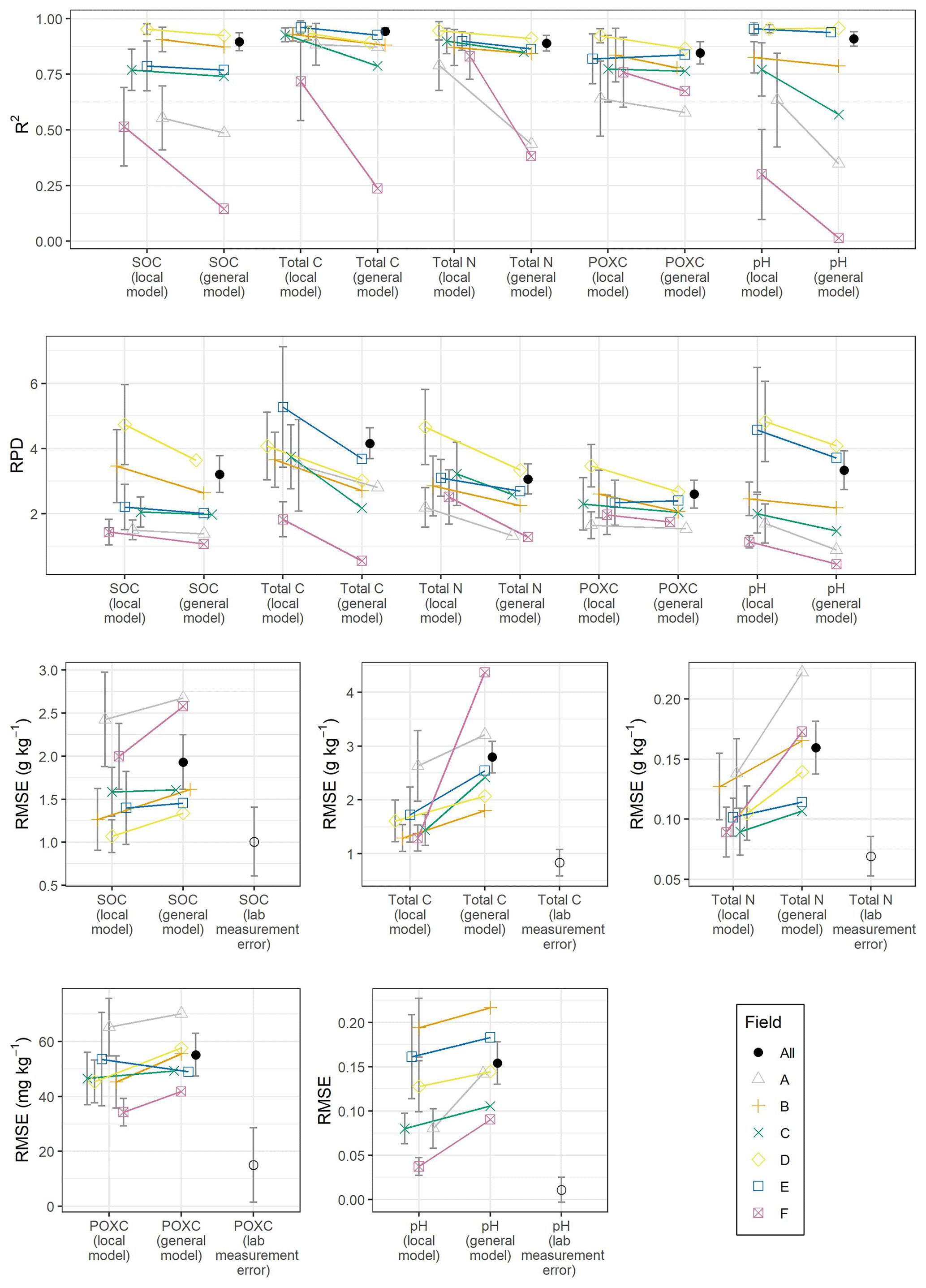
Figure 3 R², ratio of performance to deviation (RPD) and root mean square error (RMSE) calculated from the local models and field-specifically calculated from the general model for the six fields (A–F) and the five soil properties (SOC, total C, total N, POXC and pH). The error bars for the RMSE of spectral models represent standard deviations across the repeats in the cross-validation. The overall RMSE of the general model is indicated with a filled black circle and the label “All”. The RMSE values are compared with the error of the lab measurements (mean standard error of 18 triplicates indicated with standard deviation).

The field-specific RPD of the general model was, on average, 31 % lower across all soil properties compared to the local models (Fig. 3). All property–field combinations of fields B, C, D and F showed at least an approximate (RPD > 1.4) performance in the general models, whereas the seven poorly (RPD < 1.4) performing property field combinations were all from fields A and F. It can therefore be concluded that the general models could not improve the low-performing local models.

Field-specific RMSE of the general models was, on average, 47 % higher compared to the local models. However, there were substantial differences between the different fields. For field F, the field-specific RMSE values in the general models for SOC, total C, total N and pH (2.58 g kg⁻¹, 0.17 g kg⁻¹ and 0.09) were much higher compared to those of the local model (2.00 ± 0.38 g kg⁻¹, 0.09 ± 0.02 g kg⁻¹ and 0.04 ± 0.01, respectively; Fig. 3). Similarly, for total N and pH, field A had a much higher RMSE in the general model (0.22 and 0.14 g kg⁻¹) than in the local model (0.14 ± 0.03 and 0.08 ± 0.02). On the other hand, fields C and E showed quite similar RMSE values in the local and in the general model for all soil properties except total C.

The RMSE values of the best local models were close to the overall lab measurement errors for SOC, total C and total N, a bit higher for pH, and substantially higher for POXC (Fig. 3). The RMSE values of SOC for fields B (1.26 ± 0.36 g kg⁻¹) and D (1.07 ± 0.19 g kg⁻¹) were within the standard deviation of the lab measurement error for SOC (1.01 ± 0.40 g kg⁻¹). The overall lab measurement error for SOC was calculated from the measurement error for total C and inorganic C; therefore. for fields B and D, with only a little inorganic C, the lab measurement error for total C (0.83 ± 0.25 g kg⁻¹) might be the better reference. However, the RMSE of the local spectral models of all fields exceeded the overall lab measurement errors between factors of 1.1 and 2.4 for SOC, 1.6 and 3.2 for total C, 1.3 and 2.0 for total N, 2.3 and 4.3 for POXC, and between 3.4 and 17.8 for pH. The field-specific RMSE of the general model exceeded the overall lab measurement error between factors of 1.3 and 2.3 for SOC, 2.2 and 5.2 for total C, 1.5 and 3.2 for total N, 2.8 and 4.6 for POXC, and between 8.3 and 19.9 for pH.

The VIP scores (Fig. 4) show that the most important wavelengths were dataset specific. It can be seen that in field B and, to a lower extent, in field F, the same wavelengths were important in all soil properties related to soil organic matter (SOC, total C, total N and POXC), whereas in the other fields, the VIP patterns of the different properties were more distinct from each other. However, for all the analyzed soil properties, the wavelength ranges between 400 and 750 nm (visible), as well as between 1800 and 2450 nm, were most important, while the range in between was of lower importance. Nevertheless, some models had VIP scores above 2 in the range between 750 and 1800 nm.

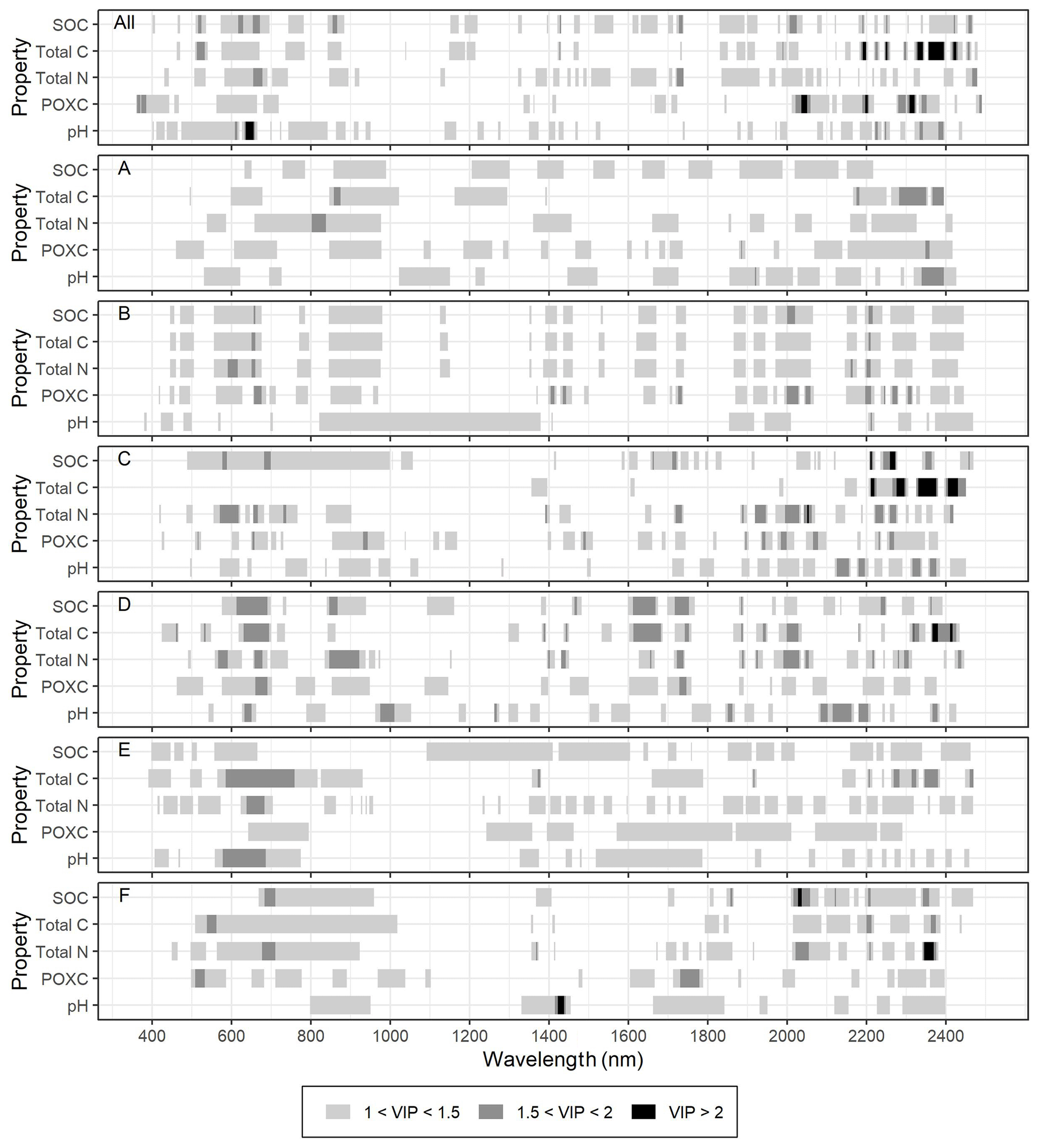
Figure 4 Variable importance in projection (VIP) for the local models of fields A–F and the general model that combined the datasets of all fields (All).

Prediction performance in terms of RMSE and RPD of total C for fields E and F was particularly lower in the general model than in the local model (Fig. 3). This finding can be explained with the VIP analysis (Fig. 4) that showed for the general model that the most important wavelength range was between 2150 and 2450 nm, while for the local models of fields E and F, it was in the range of 500 to 1020 nm. The local model for total N of field F showed very high VIP scores (> 2) in a small specific range between 2345 and 2369 nm, but these wavelengths were not important in the general model for total N (Fig. 4), which resulted in a much lower prediction accuracy of total N for field F in the general model compared to in the local model.

3.5 Site characteristics influencing model performance

We found an order of model performance with respect to R² and RPD that is dependent on mean carbonate content, the correlation coefficient between SOC and total N, and the coefficient of variation in clay content (Fig. 5). Fields A and F which showed lower model performance in terms of RPD with higher carbonate content, a lower correlation coefficient between SOC and total N, and higher variability in soil texture (compare also with density plots in Fig. 1). However, in absolute prediction performance (RMSE), we only found for SOC and pH substantial correlations ($\left|r\right|\ge \mathrm{0.46}$) between RMSE and field characteristics (Fig. 6). Compared to the three field characteristics mentioned above, we found a weaker influence of the field size; the absolute contents of sand, silt and clay; and/or the variability in the carbonate content on model performance (see Fig. S3 in the Supplement).

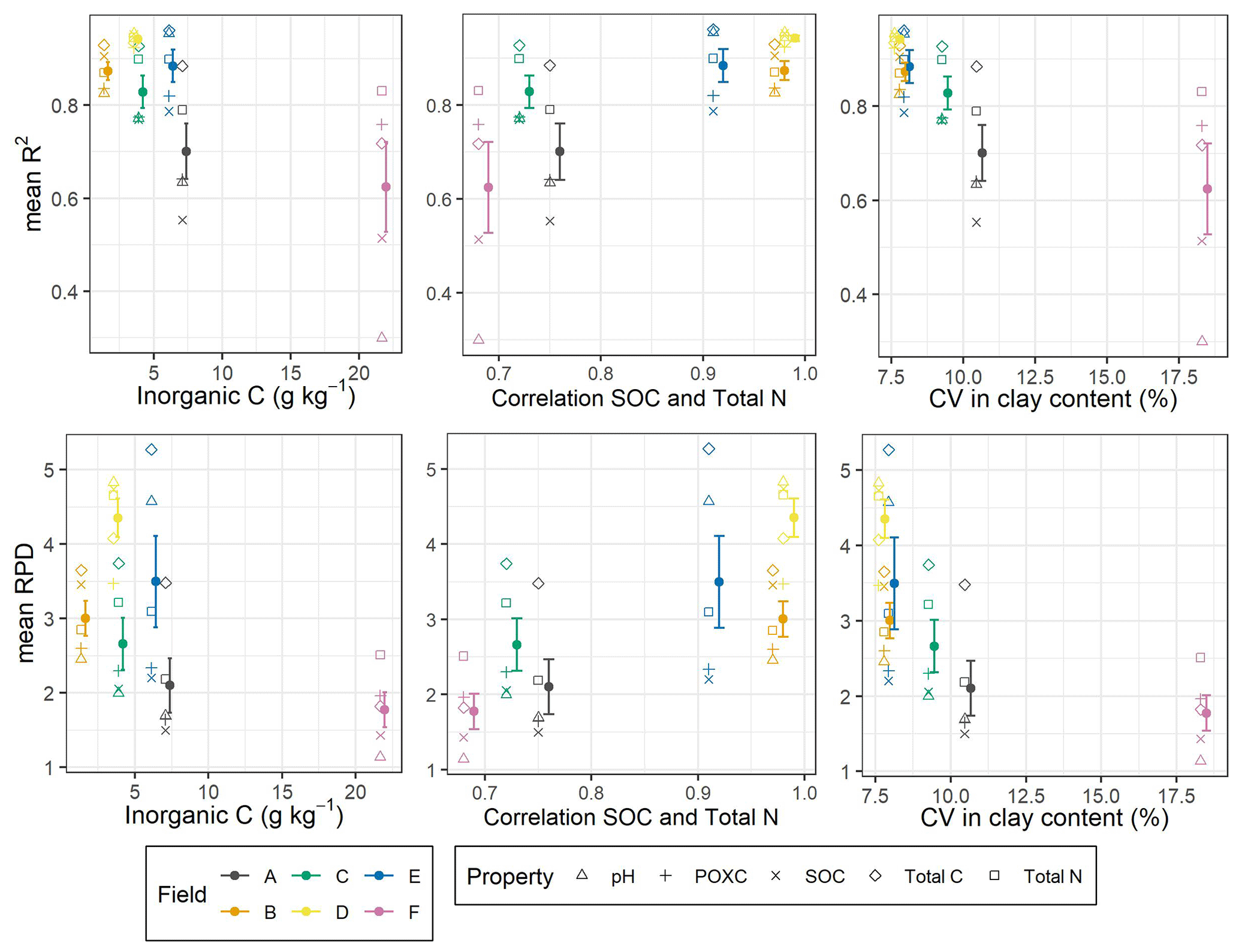
Figure 5 R² and ratio of performance to deviation (RPD) from the local models for SOC, total C, total N, POXC and pH aggregated (mean and standard error) per field (A–F) versus mean inorganic C content, Pearson's correlation coefficient between SOC and total N, and the coefficient of variation (CV) in clay content. The error bars represent standard deviations across the repeats in the cross-validation.

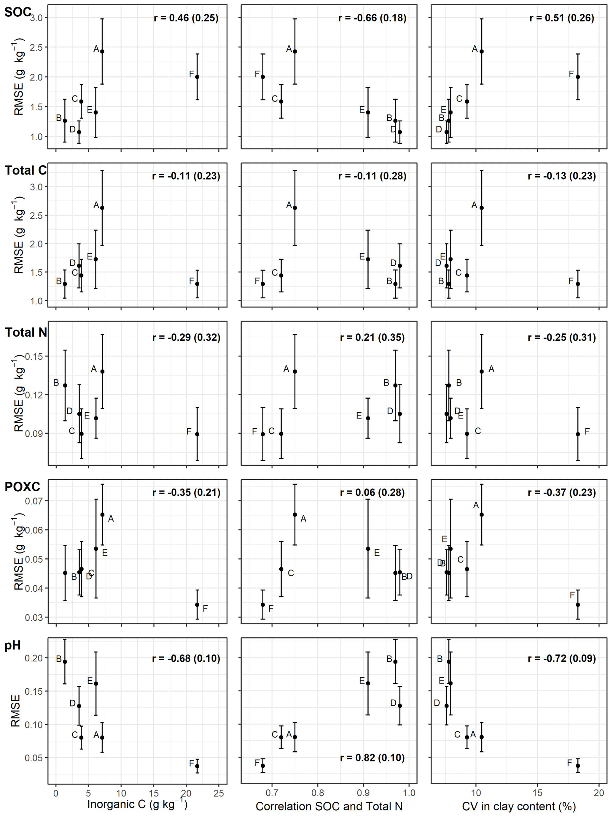
Figure 6 Root mean square error (RMSE) for the five target properties (SOC, total C, total N, POXC and pH) and each field (A–F) versus mean inorganic C content, Pearson's correlation coefficient between SOC and total N, and the coefficient of variation (CV) in clay content. The error bars represent standard deviations across the repeats in the cross-validation. Pearson's correlation coefficients are indicated as the mean and standard deviation (in parentheses) of a Monte Carlo simulation.

The influence of carbonate content on the model performance of SOC is illustrated by plotting at each wavelength the correlation coefficients between pre-processed spectral variables and inorganic C and SOC content (Fig. 7). The correlation between SOC and spectral variables was higher in fields B, D and E than in fields A, C and F, which also explains the better model performance. In field A, SOC and carbonate content show a very similar correlation with spectral variables across the whole vis–NIR range, which makes it difficult to distinguish organic and inorganic C in field A, resulting in an excellent performance of total C but much lower performance for SOC (see Table 2). Even though the correlation between spectral variables and SOC content in field C was lower than in other fields (B, D and E), the very different correlation pattern of carbonate content still resulted in good model performance for SOC. In particular, the ranges between 600 and 1200 nm and the peaks at 1680 and 2240 nm showed different spectral features for SOC and carbonate, which corresponds to the high VIP scores at those wavelengths for the SOC model in field C. In field F, correlations for both carbonate content and SOC were relatively weak, whereby carbonate content showed stronger correlations with spectral variables, which probably masked the spectral features of SOC, resulting, as for field A, in a better model for total C than SOC.

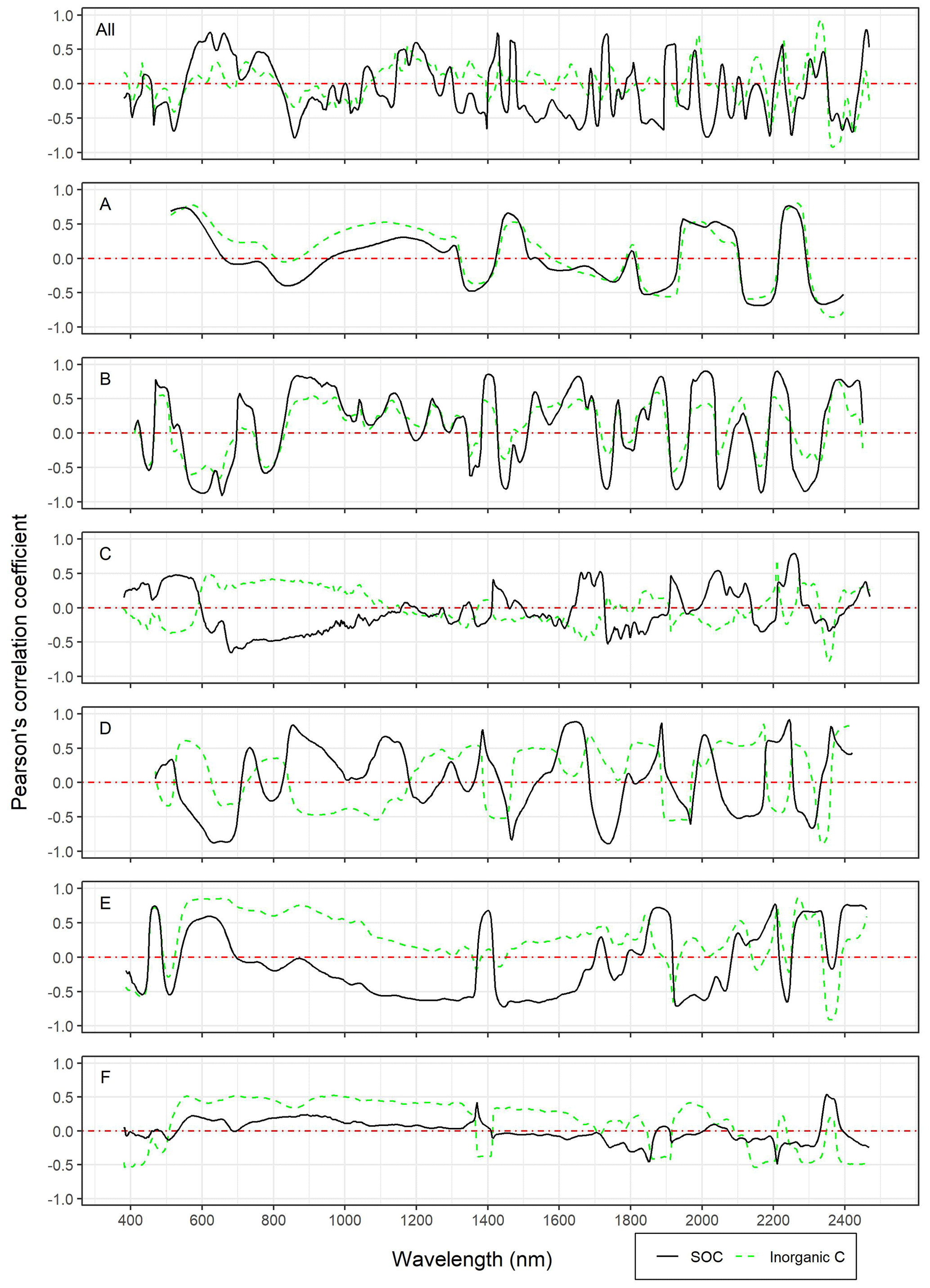
Figure 7 Correlation graphs between spectral variables at each wavelength and SOC, as well as inorganic C, for the combined dataset (All) and the individual fields (A–F). The spectra were pre-processed according to the chosen models for SOC.

The better model performance in fields B, D and E compared to in fields A, C and F also coincided with a higher correlation between SOC and total N (Fig. 5). In general, correlation coefficients between target variables tended to be higher in fields B, D and E compared to in fields A, C and F (see Fig. 8 as an example and all correlation matrices in Fig. S4 in the Supplement).

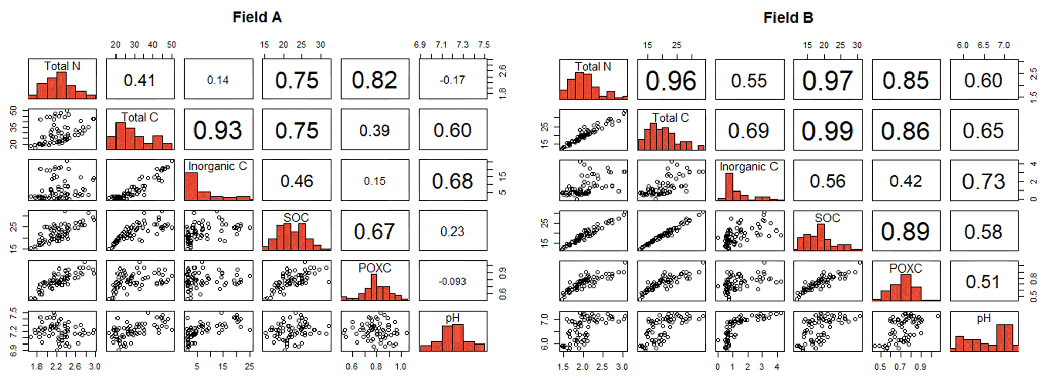
Figure 8 Pairwise correlation matrices between target soil properties and inorganic C for a field with weak correlations (field A) and a field with strong correlations (field B) between the target variables. The correlation matrices for all fields can be found in the Supplement (Fig. S4).

4 Discussion

4.1 Performance of local spectral models

Most of the developed local models showed an accurate performance and confirm the suitability of vis–NIR spectroscopy in projects of local or single-plot extent. The performance (based on RPD) of the two models for pH in fields A and F, which were classified as only approximate or even poor, respectively, can be explained by the low variability of pH in these datasets (see Fig. 1) and is supported by the fact that these two models had the smallest RMSE values for pH (Fig. 3). This explanation does not hold for the other three local models that were also classified as only approximate because SOC and POXC in field A, as well as SOC in field F, showed a similar variability compared to in the other fields (Fig. 1) but higher RMSE values. However, considering the mean SOC concentration in fields A (22.4 ± 3.7 g kg⁻¹) and F (28.6 ± 2.7 g kg⁻¹) as well as the lab measurement error (1.00 ± 0.04 g kg⁻¹), we argue that the RMSE values in fields A (2.43 ± 0.55 g kg⁻¹) and F (2.00 ± 0.38 g kg⁻¹) are probably, for many research projects, still acceptable, especially when taking into account that a higher sample size can be analyzed for the same costs.

In agreement with literature (Soriano-Disla et al., 2014), primary properties with a direct impact in the vis–NIR range, like SOC, total C, total N and POXC, showed an RMSE that was closer to the lab measurement error. On the other hand, pH has only an indirect impact on the spectra and thus showed a much higher RMSE compared to the lab measurement error. but the RMSE for pH in the local models (between 0.04 ± 0.01 and 0.19 ± 0.03) is probably small enough for most research purposes.

4.2 Comparison of general models with local models

The general models could not improve the prediction of low-performing local models. This finding is especially interesting because, in this study, the general model was built with datasets of six fields that were spatially close to one another (maximal distance of 13 km) and that had the same soil type and the same parent material. However, the base moraine as a parent material can be variable, which we mainly observed in different soil textures and carbonate contents but also in the high spectral variability (see PCA biplots in Fig. 2). In this sense, we confirm the conclusions of Seidel et al. (2019) and Ng et al. (2022), who suggested that the best solution is always to develop a local model if enough samples (> 30) are available. This conclusion is supported in this study by the quite distinctive pattern of VIP scores between the different models (Fig. 4). The overall picture shows that the wavelengths between 2000 and 2450 nm followed by the visible range between 400 and 700 nm were most important for prediction of the investigated properties, which is in agreement with the literature (Munnaf and Mouazen, 2022; Soriano-Disla et al., 2014). Nevertheless, each local model has distinct and site-specific features that could not be attributed to specific soil characteristics while being important for the model development. The development of general models where different locations are aggregated in one dataset can save costs because the number of lab analyses per location can be reduced, and less work is required for model building. Depending on the research purpose and the required measurement accuracy, the development of general models can be a very suitable and cost-effective approach. Nevertheless, this study showed that some fields (A and F) can show a poor performance in general models; hence, it is crucial to consider what locations or datasets are being combined.

4.3 Pre-processing

The selection of the optimal pre-processing scheme was crucial for model performance but was strongly dependent on the dataset. Often, MSC was the best performing pre-processing option, which was confirmed in some studies (Cambule et al., 2012; Liu et al., 2019) but disproved in others (Knox et al., 2015; Riefolo et al., 2020). We therefore highly recommend considering MSC as a pre-processing option in spectral modeling but at the same time agree with Barra et al. (2021) that there is no general pre-processing solution that works for all datasets. The principal component analysis with the combined dataset of all fields (Fig. 2) illustrates this finding by the different groupings of individual field datasets due to different pre-processing. This leads to the conclusion that studies that did not optimize the pre-processing scheme for every soil property separately did eventually not make full use of the spectroscopy, which has been shown by other studies as well (Alomar et al., 2021; Rodriguez-Febereiro et al., 2022; Singh et al., 2022). Nevertheless, the property-specific optimization of spectral pre-processing is a tedious process and constrains the fast and cost-effective application of vis–NIR spectroscopy, but some progress has recently been made by Mishra et al. (2022).

4.4 Site characteristics influencing model performance

We found higher model performance in fields with low carbonate content, high correlations between soil properties and low variability in clay content. We want to discuss how these identified important field characteristics influence or mask spectral features.

4.4.1 Mean carbonate content

We found an influence of carbonate content, with the lowest performance of local spectral models in fields A and F. Similar observations were made by Amare et al. (2013) and McCarty et al. (2002), who argued that the absorbance bands of carbonate mask those of SOC. Looking at the correlation between spectral variables and inorganic C and SOC (Fig. 7), we can confirm this finding but have to add that, on the local scale, the relative intensity of absorption bands for carbonate and SOC varied substantially between different datasets. In this context, Reeves (2010), who showed that the spectrum of a soil sample varied greatly with its carbonate content, considered the prediction of SOC in soils with high carbonate content to be one of the open questions in vis–NIR spectroscopy research. An important point missing in this discussion is the measurement accuracy of SOC in the laboratory, which is strongly influenced by the presence of carbonate and the method used (Goidts et al., 2009). If the soil samples contain carbonate, often two measurements must be conducted, and SOC is calculated as the difference between total C and inorganic C. Especially with a high carbonate content, the measurement error for the inorganic C content can be a substantial share of the SOC content. The higher lab measurement error with higher carbonate content might be a possible explanation for the lower model performance in soils with high carbonate content for SOC but not for the other four soil properties where model performance (in terms of RPD) still tended to be lower than in fields with little carbonate content (Fig. 5). This confirms the above-mentioned observation of spectral interference between inorganic C and organic matter and is additionally substantiated by the result that most properties of fields A and F showed a poor performance in the general models (Fig. 3). It is known that carbonate has many more defined peaks and less interferences with organic matter in the MIR than in the vis–NIR (Reeves, 2010). Therefore, datasets that combine soil samples with high and low carbonate content might be better predicted with MIR spectroscopy. However, while all samples of field F have a high carbonate content, field A shows a broad range of carbonate contents, whereby the mean carbonate content (7.1 ± 6.7 g kg⁻¹) is only slightly higher compared to the other fields. We therefore hypothesize that the lower performance of field A compared to fields A, B, C and D might also have additional reasons besides the field characteristics explored in this study and requires more research. The strong correlation between mean carbonate content and RMSE ($r=-\mathrm{0.68}$ ± 0.10; Fig. 6) can be explained by the very low variability in pH in fields with high carbonate content. The narrow pH ranges in these fields consequently lead to models for pH with low RMSE but also low RPD (see Fig. 5).

4.4.2 Correlations between target variables

Reflectance measured with vis–NIR spectroscopy is a combined effect of all constituents present in the soil sample (Stenberg et al., 2010), and through processing and modeling, one tries to distinguish the absorption feature of one specific soil property from the other constituents of the sample. Apart from pH, all our target variables were closely related to soil organic matter, which was, therefore, for this study, the most important soil constituent influencing the absorption features. In the case of high correlations between target variables that form part of soil organic matter, the modeling is easier because the same absorption features can be used for modeling the different properties, which was the case for field B (see VIP analysis in Fig. 4). On the other hand, a low correlation between target variables makes it more difficult to relate absorption features of organic matter to specific soil properties, which probably contributed to the lower model performance of fields A, C and F compared to fields B, D and E. The literature shows that different soil properties related to soil organic matter (e.g., SOC and total N) can show different absorption features in the vis–NIR range (Chang and Laird, 2002; Kusumo et al., 2019), which is also supported in our study (see VIP analysis in Fig. 4). However, we argue that prediction accuracy improves substantially if target variables related to soil organic matter are well correlated with each other, which was also hypothesized by Martin et al. (2002) in a one location field study.

4.4.3 Variability of clay content

Unlike Stenberg et al. (2010) and Heinze et al. (2013), we did not find a better model performance with increasing mean clay content in the dataset, which might also be explained by the relatively small range in mean clay contents of between 18 % (field F) and 38 % (field C). However, we observed that fields A and F, with lower model performance, also showed a higher variability in soil texture (see density plots in Fig. 1). We hypothesize that this observation is mainly an effect of our sampling design and the specific agricultural management and is therefore not generalizable. Clay and soil organic matter are claimed to be modeled with a high success rate with vis–NIR spectroscopy since they have strong absorption features (da Silva-Sangoi et al., 2022). Unfortunately, soil texture was measured using different samples than the reference dataset for the spectral modeling, so we cannot check for the correlation between soil texture and target variables. However, in this study, the correlation may be relatively low for the following reason: we took samples from different depths (0–5, 5–10 and 10–20 cm) within the past tillage layer and therefore expect that the soil texture is homogenized across the sampling depth. Since all fields are now under organic reduced-tillage management, the three soil layers show quite distinct soil organic matter contents (see Fig. S5 in the Supplement) but, very probably, similar soil textures. Therefore, a high (horizontal) variability in soil texture in a field (e.g., clay content) without a strong correlation to organic matter could have added “noise” to the spectrum, which worsened the prediction accuracy in our specific sampling design. Nevertheless, in untilled soils or more distinct depth segments, a high variability in soil texture may not be a disadvantage in vis–NIR modeling because it might also be correlated with organic matter.

5 Conclusions

This study investigated the impact of site characteristics on vis–NIR modeling performances and compared a local and a general modeling approach. Among the 35 models, 29 performed accurately or even excellently, whereby the RMSE was close to the lab measurement error, and achieved prediction accuracies are probably, for many research purposes, acceptable. The local models with the lowest performance were all from fields A and F, and we found three field characteristics in their datasets that interfered with model performance. Fields A and F had higher mean carbonate content, lower correlation between target soil properties and higher variability in soil texture compared to the other fields. The influence of soil texture variability was mainly an issue in this specific sampling design, whereas the influence of carbonate content and correlation between soil properties can probably be generalized due to observed spectral features and VIP analysis. Before starting a local vis–NIR project, testing for inorganic C content can be done relatively easily, but it is almost impossible to know beforehand the correlations between different soil properties. One can only be aware of the correlation issue and consider potential gradients of soil properties while designing the sampling design, which is probably more important and feasible in disturbed or agricultural soils than in natural undisturbed soils. In terms of efficiency in data collection, we conclude that, in a region, several target sites (or agricultural fields) with low carbonate contents can be combined in a general model with only a minor reduction in model performance. A general model for multiple target sites then also allows us to reduce the number of wet chemistry analyses. Whether or not several target sites with high carbonate content can be combined in one general model using vis–NIR spectroscopy is a question that requires further research. However, since carbonates show fewer interferences with organic matter in the MIR than in the vis–NIR spectral range, soil samples from sites with high carbonate content might be better predicted with MIR spectroscopy. Yet, the application of laboratory vis–NIR spectroscopy in projects of local extent provides the opportunity to increase the spatial or temporal resolution in a sampling design cost effectively with only minor decreases in measurement accuracy.