the Creative Commons Attribution 4.0 License.
the Creative Commons Attribution 4.0 License.
 | 10 Jan 2024
Thermodynamic and hydrological drivers of the soil and bedrock thermal regimes in central Spain
Jesús Fidel González-Rouco
Thomas Schmid
Camilo Melo-Aguilar
Norman Julius Steinert
Pedro José Roldán-Gómez
Francisco José Cuesta-Valero
Almudena García-García
Hugo Beltrami
Philipp de Vrese
An assessment of the soil and bedrock thermal structure of the Sierra de Guadarrama, in central Spain, is provided using subsurface and ground surface temperature data coming from four deep (20 m) monitoring profiles belonging to the Guadarrama Monitoring Network (GuMNet) and two shallow profiles (1 m) from the Spanish Meteorology Service (Agencia Estatal de Meteorología, AEMET) covering the time spans of 2015–2021 and 1989–2018, respectively. An evaluation of air and ground surface temperature coupling showed that soil insulation due to snow cover is the main source of seasonal decoupling, being especially relevant in winter at high-altitude sites. Temperature propagation in the subsurface was characterized by assuming a heat conductive regime by considering apparent thermal diffusivity values derived from the amplitude attenuation and phase shift of the annual cycle with depth. This methodology was further extended to consider the attenuation of all harmonics in the spectral domain, which allowed for analysis of thermal diffusivity from high-frequency changes in the soil near the surface at short timescales. For the deep profiles, the apparent thermal diffusivity ranges from 1 to m2 s−1, which is consistent with values for gneiss and granite, the major bedrock components in the Sierra de Guadarrama. However, thermal diffusivity is lower and more heterogeneous in the soil layers close to the surface (0.4– m2 s−1). An increase in diffusivity with depth was observed that was generally larger in the soil–bedrock transition at 4–8 m depth. The outcomes are relevant for the understanding of soil thermodynamics in relation to other soil properties. Results with the spectral method suggest that changes in near-surface thermal diffusivity are related to changes in soil moisture content, which makes it a potential tool to gain information about soil drought and water resource availability from soil temperature data.
- Article
(10423 KB) - Full-text XML
- BibTeX
- EndNote


Recent decades have witnessed substantial steps forward in knowledge of the climate system and ongoing anthropogenic climate change (Chen et al., 2021). An increase in observational datasets (Hansen et al., 2010; Lawrimore et al., 2011; Jones et al., 2012; Rohde et al., 2013; Lenssen et al., 2019; Osborn et al., 2021) and progressively more realistic climate model ensembles (von Storch, 2010; Taylor et al., 2012; Eyring et al., 2016; Maher et al., 2019) allowed the attribution of a global mean near-surface air temperature rise of more than 1 ∘C since the end of the 19th century to human activities (Chen et al., 2021; Gulev et al., 2021). This warming has been larger over land than over the ocean, with temperature values in 2011–2020 being 1.59 and 0.88 ∘C, respectively, higher than 1850–1900 (Chen et al., 2021). It is important to understand how this temperature rise has propagated into the soil and subsoil, which was shown to be important for land surface processes and meteorological extreme events (Miralles et al., 2019; Zhou et al., 2019; Seneviratne et al., 2021).
Ground surface temperature (GST) and surface air temperature (SAT) are coupled at multi-decadal and centennial scales (Pollack and Huang, 2000; Beltrami and Kellman, 2003; Melo-Aguilar et al., 2018), and GST perturbations are subsequently propagated into depth by heat transfer (Carslaw and Jaeger, 1959). A warming of near-surface soil has an impact on its biogeochemical activity (Soong et al., 2021), enhancing the metabolic activity of microorganisms, mineral weathering, and decomposition of soil organic matter (Schlesinger and Emily, 2013). It also affects soil hydrology (Krakauer et al., 2013) and increases soil respiration (Pries et al., 2017), contributing to an acceleration of the terrestrial carbon cycle (Bond-Lamberty and Thomson, 2010; Pries et al., 2017). Moreover, soil warming has relevant impacts on high-latitude regions, where permafrost thawing can produce changes in soil hydrology (Andresen et al., 2020; Burke et al., 2020) and eventually subsurface collapse (Abbott and Jones, 2015; Pegoraro et al., 2021), posing risks to infrastructure (Rotta Loria, 2023) and reshaping landscapes. Moreover, permafrost thawing triggers the release of pollutants (e.g., Schaefer et al., 2020) and massive amounts of carbon (Turetsky et al., 2019) into the atmosphere, potentially affecting the global climate (e.g., de Vrese et al., 2023). The subsurface is sensitive to not only present global warming but also to past climate changes. Deep subsurface temperatures allow recovery of past GST histories by borehole temperature profile (BTP) inversion techniques (Mareschal and Beltrami, 1992; Huang et al., 2000; Pollack and Smerdon, 2004; Jaume-Santero et al., 2016; Cuesta-Valero et al., 2022), which makes them a valuable source for climate reconstruction as far as the two fundamental hypotheses are sustained: SAT and GST changes are coupled at long-term scales and GST changes are propagated downwards by heat conduction, the main heat transfer mechanism in solids.
Support for SAT–GST coupling has been found so far from observational temperature data at some sites in North America (e.g., Putnam and Chapman, 1996; Beltrami and Kellman, 2003; Smerdon et al., 2004; Bartlett et al., 2005, 2006; Smerdon et al., 2006) and Europe (e.g., Cermak et al., 2014; Cermak and Bodri, 2016; Melo-Aguilar et al., 2022; Petersen, 2022; Dorau et al., 2022) as well as from climate simulations (González-Rouco et al., 2006; Smerdon et al., 2009; García-García et al., 2016, 2019; Melo-Aguilar et al., 2018; González-Rouco et al., 2021). These studies showed a strong coupling at long-term scales globally, with some degree of seasonal decoupling due to snow cover (Beltrami and Kellman, 2003) or changes in the surface energy balance (Smerdon et al., 2004; Melo-Aguilar et al., 2018) at regional scales. Examining whether conduction is the main heat transport mechanism in the subsurface was usually tackled by assessing the propagation of temperature perturbations and verifying that they experience an amplitude damping and phase shift with depth to an extent controlled by thermal diffusivity, a parameter that governs heat conduction processes (Carslaw and Jaeger, 1959). Previous research assessed the propagation of temperature trends (Lesperance et al., 2010) and thermal orbits (Smerdon et al., 2009) using a priori defined constant values of thermal diffusivity. Other studies tackled the propagation of single-frequency harmonic signals with depth, i.e., the annual cycle (Hurley and Wiltshire, 1993; Smerdon et al., 2003), in order to derive estimates of the apparent thermal diffusivity. Nevertheless, this approach requires continuous monitoring of subsurface temperature for at least a relatively long lapse of time (at least a few years). This was only achieved in a low number of places in North America (Smerdon et al., 2004; Bartlett et al., 2006) and Europe (Smerdon et al., 2004; Demetrescu et al., 2007; Dědeček et al., 2013; Melo-Aguilar et al., 2022). Moreover, the analysis might be hampered by potential deviations from the conductive regime in the soil near the surface due to biological, chemical, and hydrological processes (Gao et al., 2008; Tong et al., 2017). A deeper insight into the soil thermal structure is required to understand changes in its thermal properties with depth, relevant for land surface models (LSMs) and therefore with implications for land–atmosphere interactions affecting Earth system (Smerdon and Stieglitz, 2006; Ekici et al., 2014; Hermoso de Mendoza et al., 2020; Steinert et al., 2021) and forecast (Miralles et al., 2019) models. A better characterization of subsurface thermal properties can also contribute to more accurate land heat uptake estimates, i.e., energy storage in the subsurface due to industrial warming, which is the second component contributing the most to terrestrial energy partitioning (Beltrami et al., 2002; Cuesta-Valero et al., 2023; von Schuckmann et al., 2023).
This paper assesses the validity of the SAT–GST coupling and conductive thermal propagation hypotheses in the penetration of SAT perturbations into the subsurface in a high-altitude area in central Spain. This is achieved by determining the apparent soil thermal diffusivity from four short (4–6-year) and two longer (ca. 20-year) subsurface temperature records obtained at six sites in the area of the Sierra de Guadarrama and studying temperature variability in time and depth through the soil and down to the first meters of bedrock. The dataset presented in this work is unique since it gathers shallow and deep subsurface information (down to 20 m) from different sites and sensors in a high-mountain area. The complex orography of the Sierra de Guadarrama was shown to dominate the spatial mean and variability of SAT, while temporal variability was found to be very homogeneous over the region (Vegas-Cañas et al., 2020). In a first stage, we explored the SAT–GST coupling at different sites, considering the influence of processes at seasonal timescales. The propagation of the annual wave with depth was subsequently studied. This allowed us to test the conductive hypothesis and to establish a comparison between different sites by using the standard approach of focusing on the propagation of the annual wave with depth. The analysis was further extended by assessing changes in thermal diffusivity in the subsurface temperature profile, which were linked to the soil–bedrock mineral composition transition observed from samples extracted at each of the sites.
The study of the conductive regime also explored changes in apparent thermal diffusivity with time. This was feasible for the longer records for which the analysis can be performed, focusing on different multi-annual temporal intervals. This approach was however hampered by the short time span of observations at most sites considered herein. This problem was overcome by introducing a new method that makes use of the information in the spectral domain. Instead of considering only the annual cycle, the propagation of the complete range of harmonics of different frequencies that contribute to temperature variability was used. This allowed for focusing on intra-annual timescales and using shorter time series to estimate soil thermal diffusivity near the surface. The fact that apparent thermal diffusivity values can be retrieved from shorter time spans also allowed diffusivity changes to be evaluated through time and connected to changes in soil moisture content (Sorour et al., 1990; Fuchs et al., 2021).
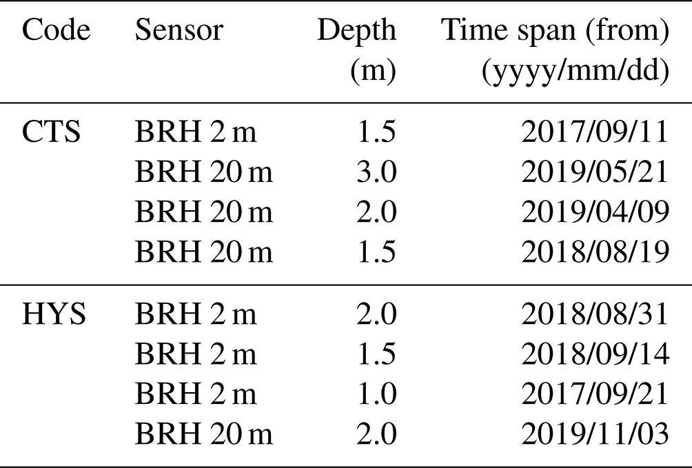
Table 1Name, code, coordinates (longitude, latitude), altitude, and time span of available subsurface temperature data at both the GuMNet and AEMET observational sites.
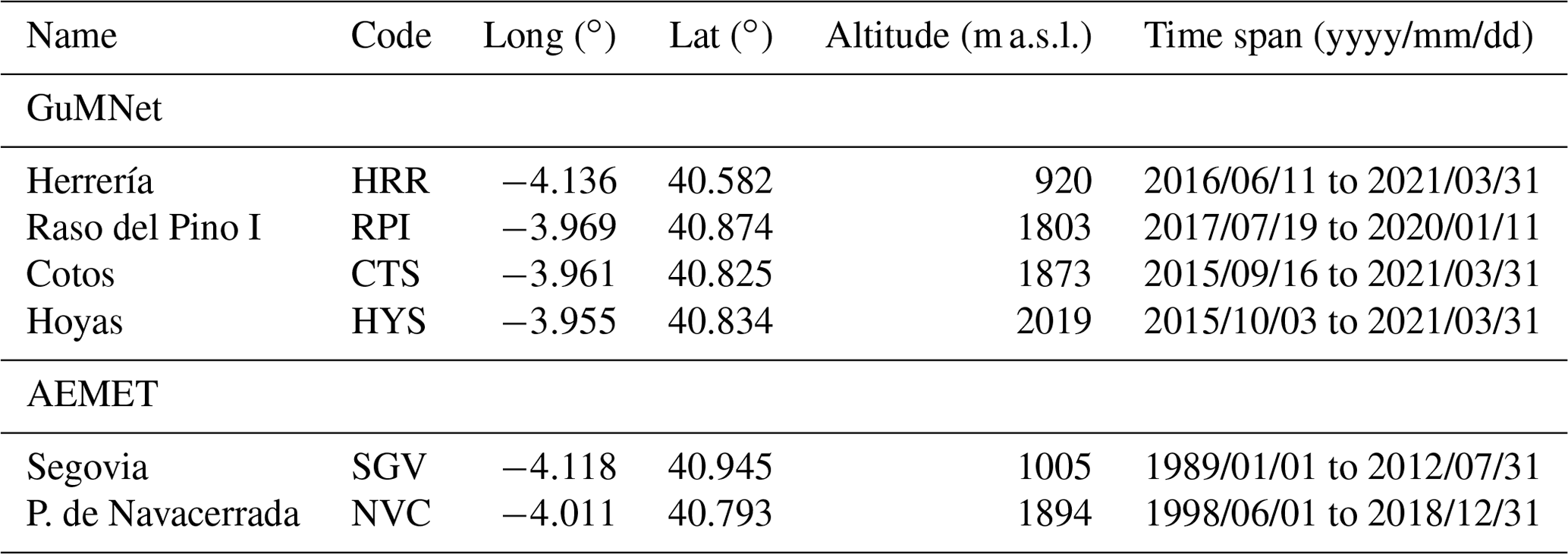
The subsurface data analyzed hereinafter consist of temperature time series from six locations distributed over the Sierra de Guadarrama. Table 1 includes a more detailed description of the name, code, geographical position, and date range of available data of each location. The Sierra de Guadarrama is part of the Sistema Central, a mountain system that splits the Spanish Central Plateau into a southeastern side, with altitudes of around 600 m a.s.l. (above sea level), and a northwestern side, of higher elevation (ca. 750 m a.s.l.). Elevations in the sierra span from 900 at the foothills to ca. 2200–2400 m a.s.l. at the summits. Two sites, Puerto de Navacerrada and Segovia, belong to the Spanish Meteorological Service (Agencia Estatal de Meteorología, AEMET), and the rest are part of the Guadarrama Monitoring Network (GuMNet). The latter was created in 2014 with the aim of gaining further insights into climate variability in mountain environments in central Spain (Vegas-Cañas et al., 2020). GuMNet consists of 10 atmosphere and subsurface monitoring stations, which cover a vertical gradient ranging from 900 to 2200 m a.s.l., spreading over the mountainous terrain of the Sierra de Guadarrama. In this work, four stations were selected that provide information on atmospheric variables and subsurface temperatures (Fig. 1a). In all the cases, vegetation cover at the sites consists of short grass that changes minimally during the year. No site has trees or shrubs within the fenced perimeter of the monitoring station.
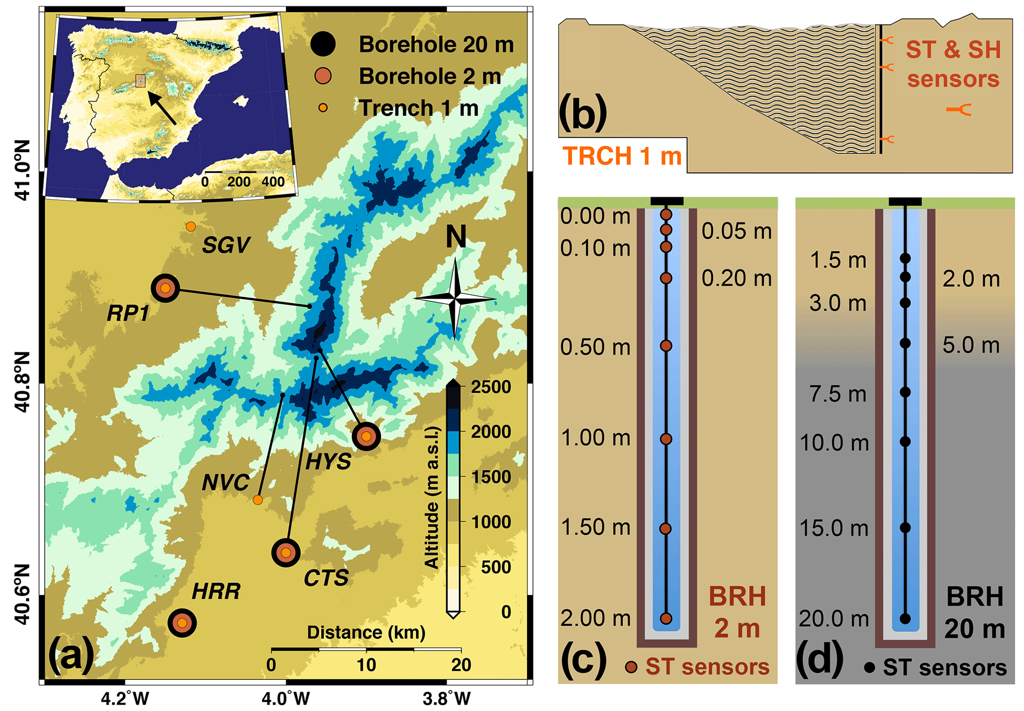
Figure 1(a) Subsurface data availability over the area of the Sierra de Guadarrama used in this work. The map in the inset (upper-left corner) shows the location of the Sierra de Guadarrama in the Iberian Peninsula. The extension covered by the map in panel (a) is represented by the orange-shaded area in the inset. Right: conceptual sketches of subsurface equipment for 1 m trenches (b), 2 m (c), and 20 m boreholes (d). The same distribution of subsurface temperature (referred to as ST in the figure) sensor depths is carried out at every site (c, d). Sensors in trenches are unevenly placed within the first meter of the ground at different sites. Pale yellow (grey) background color refers to soil (bedrock) in all the panels. The transition depth between soil and bedrock (blurred area in panel d) is only intended for illustration and takes place at different depths for each site. Colors and shapes of the symbols are also illustrative. In addition to subsurface temperature data, all the stations provide SAT measurements as well as soil moisture content (referred to as SH in the figure) in the trenches.
The subsurface thermal regime is monitored by two different arrangements. Near-surface soil temperatures are measured at various levels in trenches (TRCH; Fig. 1b) at all the sites. Trenches are excavations forming a slope in which the frontal wall was used to analyze the vertical structure of soil horizons (Brady and Weil, 2017) and to insert soil temperature reflectometer sensors down to a depth of about 1 m. Trenches were refilled with the previously extracted material. Deeper temperatures in the soil and bedrock are monitored within cased boreholes. They consist of a small diameter (ca. 76 mm) cylindrical drill in depth where a casing was inserted and afterward filled up with a silicone gel. Temperatures therein are measured with calibrated platinum resistance thermometers embedded inside the casing (BRH; Fig. 1c, d). For the sake of having a finer vertical resolution in the soil near the surface and some level of redundancy, two boreholes were installed at these sites: a deep one going down to 20 m (BRH 20 m in Fig. 1 and Table 2) and a shallow one of 2 m (BRH 2 m in Fig. 1). Table 2 provides a detailed list of the depths at which subsurface temperature sensors were installed. Levels with malfunctioning sensors are marked with a dash.
Table 2Depths corresponding to the available individual temperature series in the trenches and boreholes at each of the sites used in this work (see Table 1 for the codes). Dashes indicate missing data due to sensor malfunction.
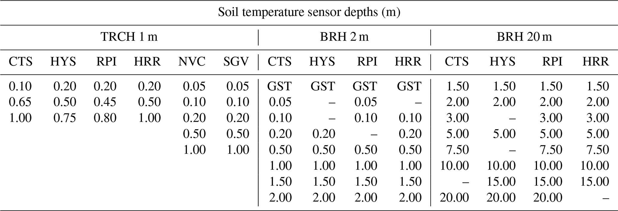
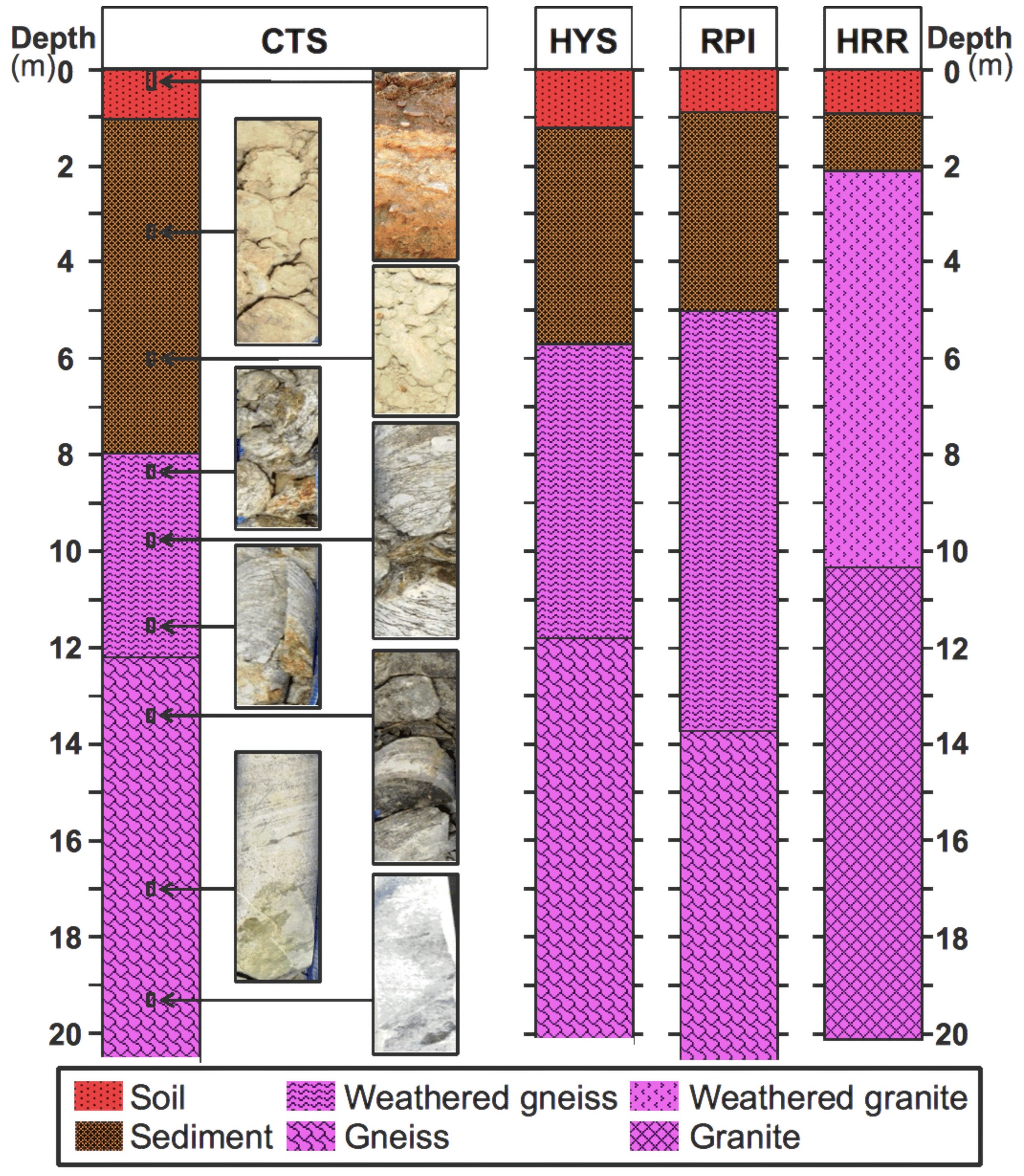
Figure 2Subsurface mineral composition of the borehole cores extracted when drilling at CTS, HYS, RPI, and HRR. The top soil layer (red) covers approximately the first soil meter at every site, whilst sediment (brown) depth varies from one site to the other. Bedrock (magenta) underneath is gneiss or granite, normally weathered at the top. In the case of CTS, some photos of the material at different depths are also included for illustration.
During the borehole drilling process at the GuMNet sites, the extracted cores were preserved. They were subsequently sampled and characterized. The result is shown in Fig. 2, where the limits between the soil, sediment, and rock layers were determined. The superficial soil layer is made up of different soil horizons (Brady and Weil, 2017) containing an O and/or A horizon (i.e., topsoil) followed by E and/or B (i.e., subsoil) and several C (i.e., parent material) horizons that reach a depth of approximately 1 m. The underlying sediment layer contains eroded material of loose debris rocks that have accumulated at the corresponding locations. The Cotos (CTS), Hoyas (HYS), and Raso del Pino I (RPI) profiles are located over gneiss rock and Herrería (HRR) on granite rock. In all the profiles, the upper layers have weathered bedrock, and with depth this bedrock is unweathered and compact. This information was used in Sect. 4 to compare changes in apparent thermal diffusivity to changes in mineral composition and textures with depth.
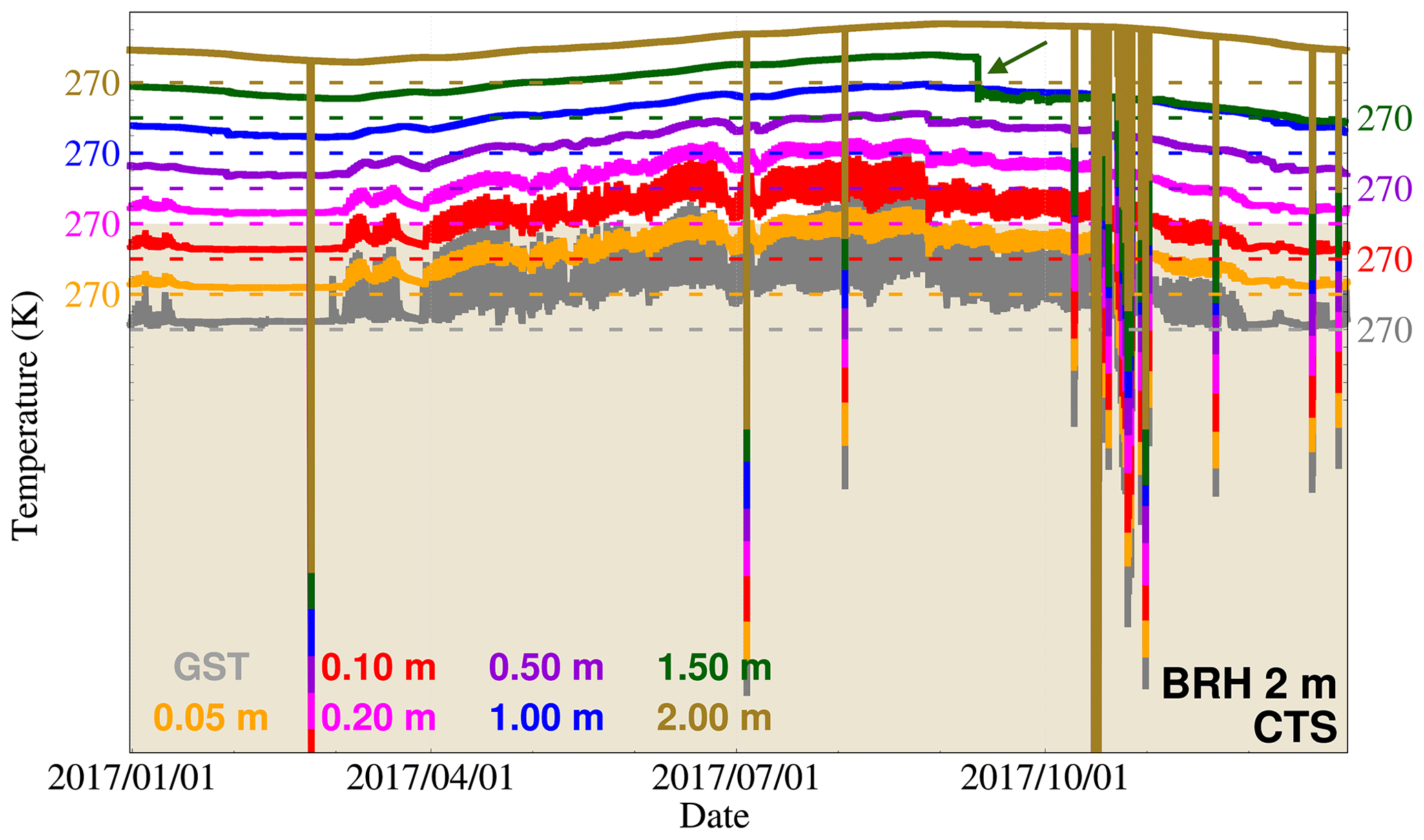
Figure 3Example of errors in BRH 2 m at CTS in the year 2017. The 10 min GST observations (grey) and those of temperatures for seven levels below the surface are shown. Time series are shifted an offset equivalent to 10 K and ticks are included every 5 K for clearer visualization. The value of 270 K is shown for all levels as a reference. The olive-colored band at the bottom represents the level of 230 K for the 2 m depth temperature time series used to determine nonphysical values. The segment of the level of 1.5 m shown by the arrow indicates a shift in the mean temperature value. Time values after the shift are subsequently eliminated.
Subsurface temperature measurements are taken at a 10 min time resolution at every GuMNet station. As a first step prior to the analysis carried out in this work, subsurface data were subjected to quality-control and resampling procedures. AEMET stations Puerto de Navacerrada and Segovia (NVC and SGV) were independently processed and resampled to daily resolution as described in Melo-Aguilar et al. (2022). The quality control of GuMNet sites focused first on removing data outliers. Since subsurface temperature sensors are connected in series in both boreholes and trenches (see Fig. 1b–d), most often erroneous extreme values are recorded at all levels simultaneously. Thus, to avoid discarding values that might be correct meteorological extremes, this correction was applied for both boreholes and trenches using the deepest time series to detect the erroneous values. The lowermost level was used because it shows the lowest temperature variability due to conductive damping of the surface signal. This reduces the range of high-frequency variability in the series except for the erroneous data, which makes non-reliable outliers easier to detect (Fig. 3). First, outliers flagged as physically implausible were removed, i.e., values falling below 230 K or exceeding 350 K. The detection of outliers below 230 K can be considered redundant since the next step would have detected all the values lying beneath this threshold. Second, the remaining spikes were flagged and discarded. Spikes were detected by calculating the sequential differences of each value minus its preceding one and screening the values in the interval , where Q1, Q3, and IQR are the first and third quartiles and the interquartile range of the distribution of temperature differences (Tukey, 1977). Time steps whose difference values were missing or outside of the screening interval were removed. Figure 3 shows an example of such spike screening for the BRH 2 m at CTS. The outliers depict coinciding failures at all the levels. The procedure is very conservative as the bottom levels have very low temperature variability and all spikes are identified and removed at each level. Note the decrease in high-frequency variability with subsurface depth, which is consistent with a heat conduction process (Carslaw and Jaeger, 1959). Once outliers were removed, time series were subjected to a one-by-one inspection, and periods with clear drifts or strong changes in variability were manually removed (check Table 3 for a list of removed periods at CTS and HYS). Figure 3 also shows an example of one such period for the 1.5 m depth temperatures at CTS (green arrow).
Table 3Record of periods discarded at CTS and HYS for the analysis subsequently performed in this work. Records are sorted by log depths (descending) and span from the dates indicated up to the present.
After applying the aforementioned quality-control procedures, the GuMNet series were resampled at hourly resolution, which filtered out noisy intra-hourly variability unnecessary for the subsequent analysis of the data. This was attained by calculating pseudo-hourly time series, which was carried out with a nearest-neighbor resampling technique (Brandsma and Können, 2006) by selecting the 10 min data closest to the hour. Finally, the resulting series were averaged to obtain daily mean subsurface temperatures that were subsequently used to analyze the propagation of the annual cycle.
In addition to subsurface temperature data, all the stations include SAT measurements as well as soil moisture content within the trench-monitoring levels. SAT is recorded at 2 m above the ground surface at all the sites using a temperature probe encapsulated within a shield. Snow cover data are also available at CTS, HYS, and RPI (see the codes in Table 1). Snow depth is measured with an ultrasonic snow depth sensor that captures the distance to the surface. Depth values are obtained from the subtraction of the surface level measured from the reference ground surface level value. These additional data were used to explore potential drivers of the SAT–GST seasonal decoupling and temporal changes in soil apparent thermal diffusivity at some sites.
The SAT–GST seasonal coupling was explored by quantifying the offset and correlation of seasonal (December–January–February, DJF; June–July–August, JJA) and annual temperatures at 2 m above the ground surface with GSTs taken from the top-level temperatures in the BRH 2 m setup. The estimates were obtained from the complete time span of available data at each site (Tables 1 and 2).
Furthermore, the subsurface temperature distribution was analyzed by assuming that GST perturbations are propagated downwards by heat conduction. Considering that every level is at a thermal equilibrium state, horizontal heat transport may be neglected. Thus, the problem is reduced to resolve the one-dimensional time-dependent heat conduction equation, . If GST is assumed to follow a sinusoidal (e.g., annual) cycle, subsurface temperatures at any depth z can be derived as follows (Hurley and Wiltshire, 1993; Smerdon and Stieglitz, 2006):
where T0 and A0 are the mean temperature and wave amplitude of the annual cycle at the ground surface, respectively, fa is the frequency of the annual cycle, and α is the thermal diffusivity, which is a direct function of thermal conductivity (k) and the inverse of density (ρ) and heat capacity (c), i.e., . Equation (1) shows that the annual cycle amplitude is attenuated and phase-shifted with depth. The amplitude attenuation is exponential, and the phase shift is linear with depth and dependent on the thermal diffusivity; i.e., increasing this parameter produces both a greater amplitude attenuation and a phase shift.
Amplitude and phase values of the annual cycle at every level were obtained by least-squares fitting subsurface temperature series at a daily resolution to an annual-period sinusoidal wave. Then, linear regression analysis of the annual-cycle amplitude (phase-shift) values with depth yielded estimates of the apparent thermal diffusivity of the subsurface, since the resulting slope is equal to in Eq. (1). Amplitude and phase-shift values coming from every installation (TRCH 1 m, BRH 2 m, and BRH 20 m) were independently adjusted and normalized to prevent any disruption due to blending data from different sources when assessing heat propagation from the ground surface to 20 m depth. Normalization was achieved by dividing the amplitude values of the annual cycle at every level by the amplitude value at the ground surface and by subtracting the phase-shift value at the ground surface from the phase-shift values of the annual cycle at every level. The values at the ground surface were obtained through a linear regression adjustment. Once normalized, all amplitude and phase-shift values were brought together and linearly adjusted to obtain a single estimate of thermal diffusivity for the whole subsurface profile at every station. A similar methodological approach based on the analysis of the annual cycle has been widely used in the literature (e.g., Smerdon et al., 2004; Pollack et al., 2005; González-Rouco et al., 2009), and it will be referred to as the classic analytical approach (CA) hereafter. This CA framework was also used to estimate changes in apparent thermal diffusivity with depth, either by considering changes between pairs of subsurface levels or by identifying depths where significant changes in apparent thermal diffusivity occur. This was achieved using a two-phase regression analysis (Solow, 1987, 1995; Melo-Aguilar et al., 2018), which determines whether there is a change point for which linear fits to the segments before and after the change point significantly improve the results compared to a linear fit to the complete curve.
Beyond the regular nature of the annual cycle, GST variability encloses perturbations at different frequencies. If GST is considered a sum of temperature harmonics, each harmonic is also propagated with depth following Carslaw and Jaeger (1959):
where fi is the frequency of each wave component in a spectral decomposition, as yielded by a Fourier periodogram for instance (Brigham and Morrow, 1967). Equation (2) shows that amplitude attenuation and phase shift are frequency-dependent. More precisely, amplitude attenuation grows exponentially with frequency; i.e., high-frequency harmonics decay more intensively with depth, whilst low-frequency perturbations can propagate more deeply. For instance, the daily cycle hardly reaches a depth of 50 cm, while the annual cycle propagates down to 15 m (Putnam and Chapman, 1996). The temperature spectral attenuation with depth can be expressed as
where PGST(ω) and Pz(ω) are the spectral power densities of GST and that at a given level z, respectively:
where Ns is the temporal resolution of the temperature time signal at z, T(z,t); f is the frequency; and ω is the angular frequency of the different wave components of T(z,t). In order to minimize the undesirable effect of Gibbs' noise at high frequencies, P was calculated by making use of Welch's modified periodogram (Stoica and Moses, 1997). Because the periodogram calculation requires evenly spaced data, data gaps were previously filled by linear interpolation. As the spectral attenuation must follow an exponential relationship with frequency, the spectral amplitude attenuation curves attained from the analysis of Eq. (3) were subsequently linearized (i.e., taking the natural logarithm) and linearly fitted by least squares to the values obtained at all available depths:
Estimates for the apparent thermal diffusivity of the soil layer in between the ground surface and level z can be retrieved by dividing πz2 by the regression line slope, , in Eq. (5). To prevent poor signal-to-noise ratios at high frequencies from biasing the analysis, amplitude attenuation values at frequencies higher than the corresponding e2-fold decay cut-off frequency (i.e., spectral harmonics attenuated more than e2 times) were filtered out at every level. To determine this frequency at every site and level, near-surface soil thermal diffusivity values coming from the CA are used. However, it is possible to use a physically plausible prior thermal diffusivity value (ca. 10−6 m2 s−1) to calculate this frequency, leading to very similar results and thus making the spectral method (SpM) independent of the CA. This alternative approach to the CA will from now on be called the SpM. While the CA needs at least a few years of data to provide reliable fits of the annual cycle to subsequently retrieve the apparent thermal diffusivity, the SpM can be applied to data at shorter time intervals. This makes it suitable for analyzing short time series, which is the case with some of the time series presented in this work. Consequently, the SpM was used in this work to retrieve apparent thermal diffusivity values in the first meter of the soil at every station. These values were then compared to the estimates coming from the CA to assess the robustness of the results from both methods. Furthermore, the SpM allows some insight into short-term changes in soil apparent thermal diffusivity and its potential relation to changes in snow cover and soil moisture content.
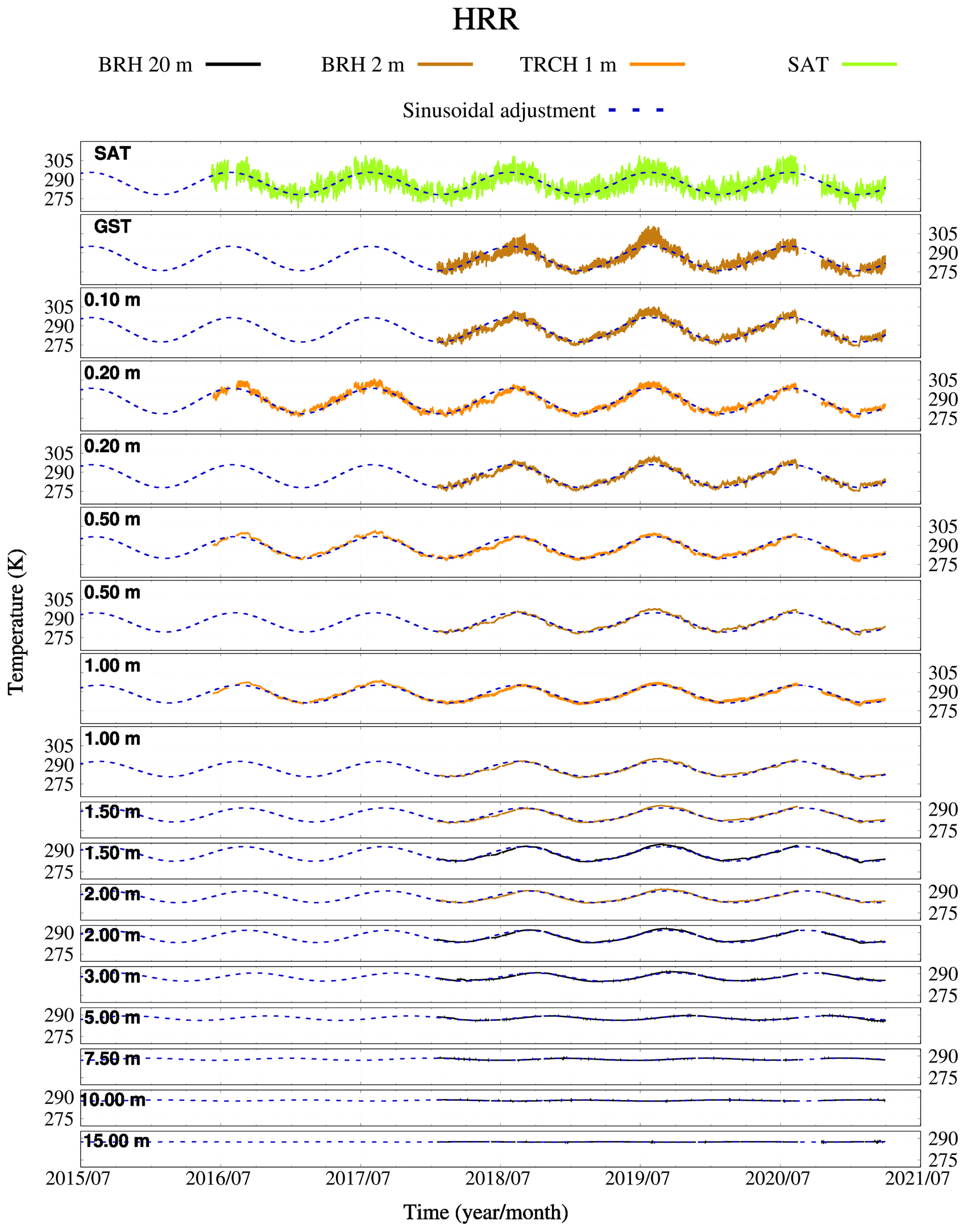
Figure 4SAT, GST, and subsurface temperatures (K) at HRR. Subsurface temperatures stem from the BRH 20 m (black lines), BRH 2 m (brown lines), and TRCH 1 m (orange lines). Blue dashed lines show the resulting fit to an annual cycle at each depth.
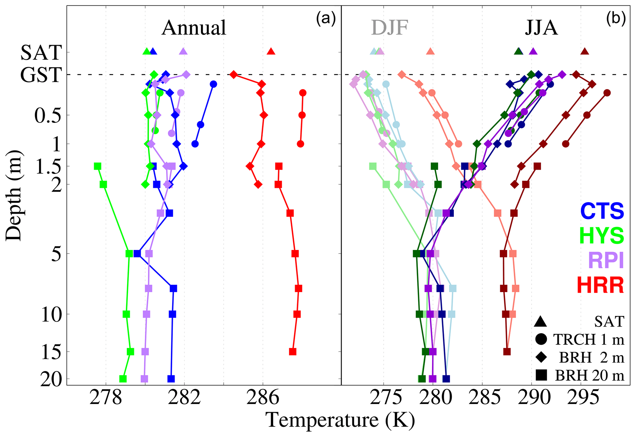
Figure 5SAT (triangles) and subsurface temperature profiles (continuous line with diamonds for BRH 2 m, squares for BRH 20 m, and circles for TRCH 1 m) at CTS (blue), HYS (green), RPI (purple), and HRR (red) for their respective whole time spans (see Table 1). Annual mean temperatures are shown on the left-hand side of the figure, whilst JJA (DJF) is shown on the right in dark (light) colors.
4.1 Temperature variability at the ground surface
In order to illustrate the amplitude attenuation and shift with depth, Fig. 4 compiles all the subsurface temperature series at hourly resolution coming from BRH 20 m, BRH 2 m, and TRCH 1 m at HRR; SAT is also represented to illustrate the coupling at the surface. A first inspection reveals that the only regular temperature variation at all levels, in both timing and magnitude, is the annual cycle. The daily cycle, while regular in occurrence, changes a lot in magnitude due to weather conditions and seasonality. The annual cycle is most prominent at the ground surface (ca. 9 K amplitude) despite the fact that both SAT and GST also show remarkable daily temperature variations (ca. 4 K amplitude). It is noteworthy how the annual cycle decreases in amplitude with depth to be imperceptible at 15 m, where annual temperature variations are on the same order as the accuracy of the sensor, i.e., 0.1 K. Furthermore, the increasing lag in the occurrence of temperature maxima in summer and minima in winter are indicative of the phase shift due to conductive propagation of the temperature variations. Both phenomena can be inferred by observing either the subsurface temperature series or the sinusoidal curves adjusted to an annual cycle (blue dashed lines). Moreover, SAT and GST daily variabilities are similar during the year except in winter, when GST variability is smaller in comparison with SAT. For other soil levels, warm or cold anomalies that last a few weeks are propagated only in the first meter of the soil.
The long-term mean temperatures with depth for CTS, HYS, RPI, and HRR are shown in Fig. 5. The annual vertical mean temperature of the profile, which is observed below the depth at which the annual cycle has been attenuated (ca. 15 m), is remarkably higher at HRR (286.8 K) than at CTS (281.3 K), HYS (279.2 K), and RPI (280.9 K). The JJA and DJF temperature profiles further depict the seasonal temperature variations towards warmer values in summer and colder values in winter as well as the amplitude attenuation of these seasonal variations with depth. JJA and DJF temperature profiles converge at a depth of around 5 m at all the sites to then cross over, which is a sign of the phase shift of the annual cycle. The transition from the BRH 2 m profile to the BRH 20 m profile shows noticeable discontinuities that are on the order of 2.7 and 2.2 K at HYS and about 1.5 and 1 K at HRR for the 1.5 and 2 m temperature levels, respectively. These discontinuities are most likely due to heterogeneous soil and sediment formations. The uppermost soil and sediment layers vary according to the sites and in all cases reach a depth greater than 2 m (Fig. 2). In the case of HYS, for instance, the greatest annual temperature difference is observed between the 2 and 20 m boreholes at 1.5 m depth. The site is on a middle slope with a slope gradient of 10 % to 15 %, and the soil horizons have a sandy loam to sandy clay loam texture. What is most notable is the varying content of rock fragments (15 % to >80 %) within the different soil horizons. This is further observed throughout the sediment layer, where the rock fragment distribution varies with depth and is very weathered. Therefore, temperature variations over short distances and within the uppermost soil and sediment layers are expected due to their different properties, which will also influence the water infiltration and circulation. With regard to SAT–GST coupling, Fig. 5 shows that the annual cycle is less pronounced for SAT than GST due to radiative warming and cooling of the ground surface, resulting in a negative SAT–GST offset in summer and a positive one in winter. The distribution of SAT and GST mean values of the sites agrees with their different altitudes, which yields a vertical gradient of −5.81 K km−1 in SAT given by Vegas-Cañas et al. (2020) for the area of the Sierra de Guadarrama. SATs in Fig. 5 comply well with this value, rendering a gradient of −6.55 K km−1, which is larger in magnitude due to this subset of sites being distributed over the higher altitudes of the region. Subsurface temperatures with depth follow the distribution of SAT at HYS and HRR, with HRR exhibiting higher values for the whole profile. However, this pattern is not observed at RPI and CTS, as RPI shows lower temperatures below 5 m despite SAT and GST being warmer, which might be due to processes within the soil that have not been further investigated in this paper.
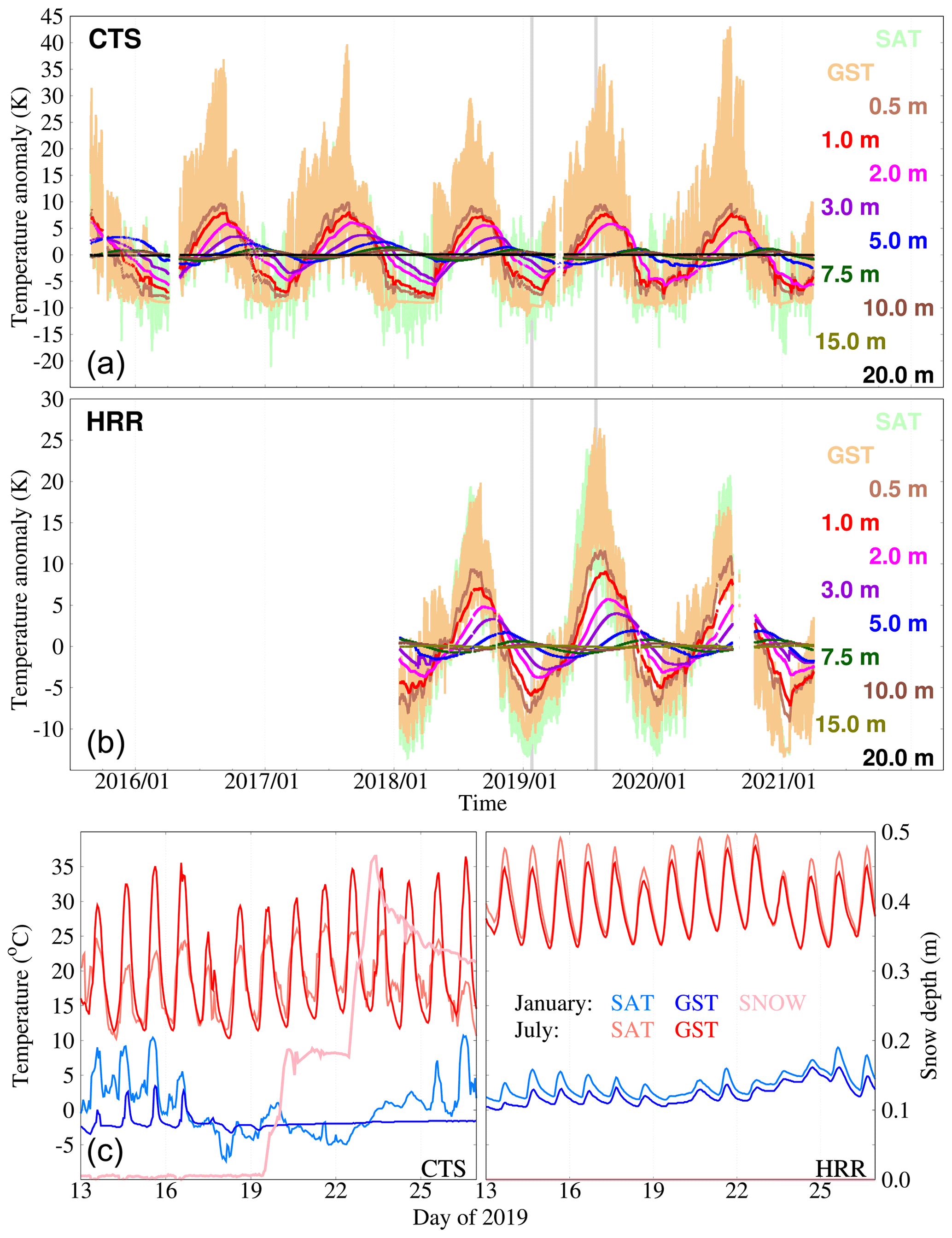
Figure 6SAT, GST, and subsurface temperature anomalies (K) with respect to the annual mean at CTS (a) and HRR (b). (c) SAT (light) and GST (∘C; dark colors) changes during 10 d in January (blue) and July (red) 2019 and the evolution of the snow cover (m; light pink) at CTS and HRR.
Temperature anomalies with respect to the long-term mean at each depth are shown in Fig. 6 as an example for CTS and HRR. This allows for a clearer visualization of the amplitude attenuation and phase shift with depth. Two cycles are clearly identified again at both sites: the daily cycle, which is visible at GST and hardly noticeable at 0.5 m (Fig. 6a, b), and the annual cycle, with an amplitude reduction and phase shift that are traceable down to 15 m. Nevertheless, there are two differences that are worth mentioning. On the one hand, GST and subsurface temperatures underneath at CTS show some constant signal time periods in winter that are not found in SAT, as shown in Fig. 6c, where SAT and GST are represented for a shared period in January 2019 at CTS and HRR. As soon as a snow layer emerges at CTS on 19 January 2019, GST oscillations are suppressed despite SAT still varying. This is due to the combination of the soil-insulating effect of snow cover (Bartlett et al., 2005; Zhang, 2005) and the zero-curtain effect, which prevents temperatures at the ground surface from dropping far below zero due to latent heat release (Outcalt et al., 1990). This behavior is not shared by HRR, since at this lower altitude a regular seasonal snow layer is less frequent. Hence, HRR is snow-free during the same dates, so SAT and GST variations are strongly coupled. On the other hand, note that SAT variability differs from one site to the other, with the amplitude of the daily cycle greater and the annual cycle smaller at CTS than at HRR, as illustrated by greater differences in SAT variations in July 2019 with respect to those in January 2019. This is consistent with SAT annual variability decreasing and intra-annual increasing with altitude in the same area, as shown by Vegas-Cañas et al. (2020).
Table 4SAT–GST differences in the mean (K) and Pearson's correlation coefficient using daily data. The annual wave was previously filtered out from both SAT and GST data for this analysis. Non-significant (p<0.05) differences and correlations are shown in bold.
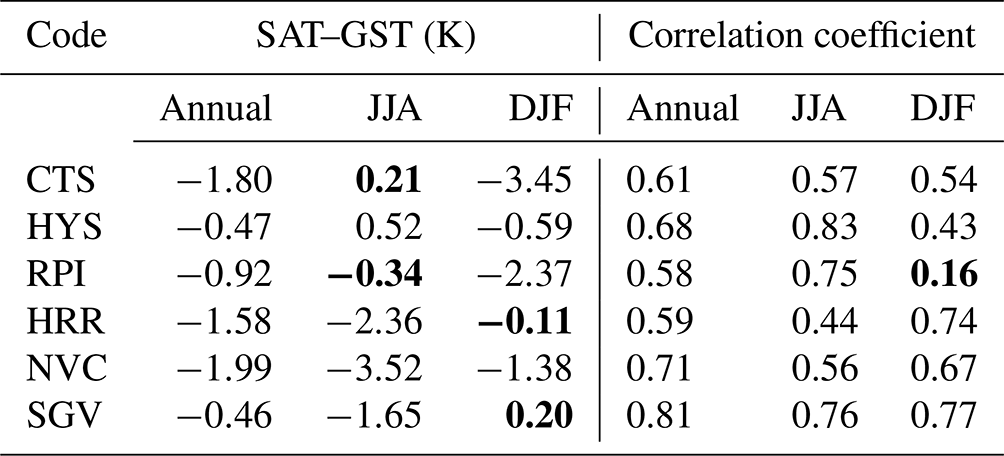
Air–ground temperature seasonal decoupling is further explored in Table 4, where SAT–GST differences and Pearson's correlation coefficient were computed after filtering out the annual cycle. SAT–GST differences show that, on average, GST is warmer than SAT, with annual differences being negative. Correlations using daily data are all significant (p<0.05, Student's t test) and above 0.58 for all the sites. Differences tend to be larger during DJF, likely due to the insulating effect of snow cover, which hampers soil cooling and disrupts SAT–GST coupling. During JJA, significantly warmer GSTs are found at HRR, NVC, and SGV, likely due to surface radiative warming. Additionally, correlation analysis yields the weakest values in DJF at the highest-altitude sites, i.e., RPI, HYS, and CTS, which may be linked to the presence of a steadier seasonal snow layer than at the lowest sites. Low correlation is found in JJA at HRR, which might be due to weaker latent heat fluxes connected to Iberian soils' summer drought (Vicente-Serrano et al., 2013). Nevertheless, the diverse local responses at the various sites could be due to land cover differences, water or latent heat exchanges, or other factors (Cermak and Bodri, 2016; Cermak et al., 2017) that have not been further examined herein.
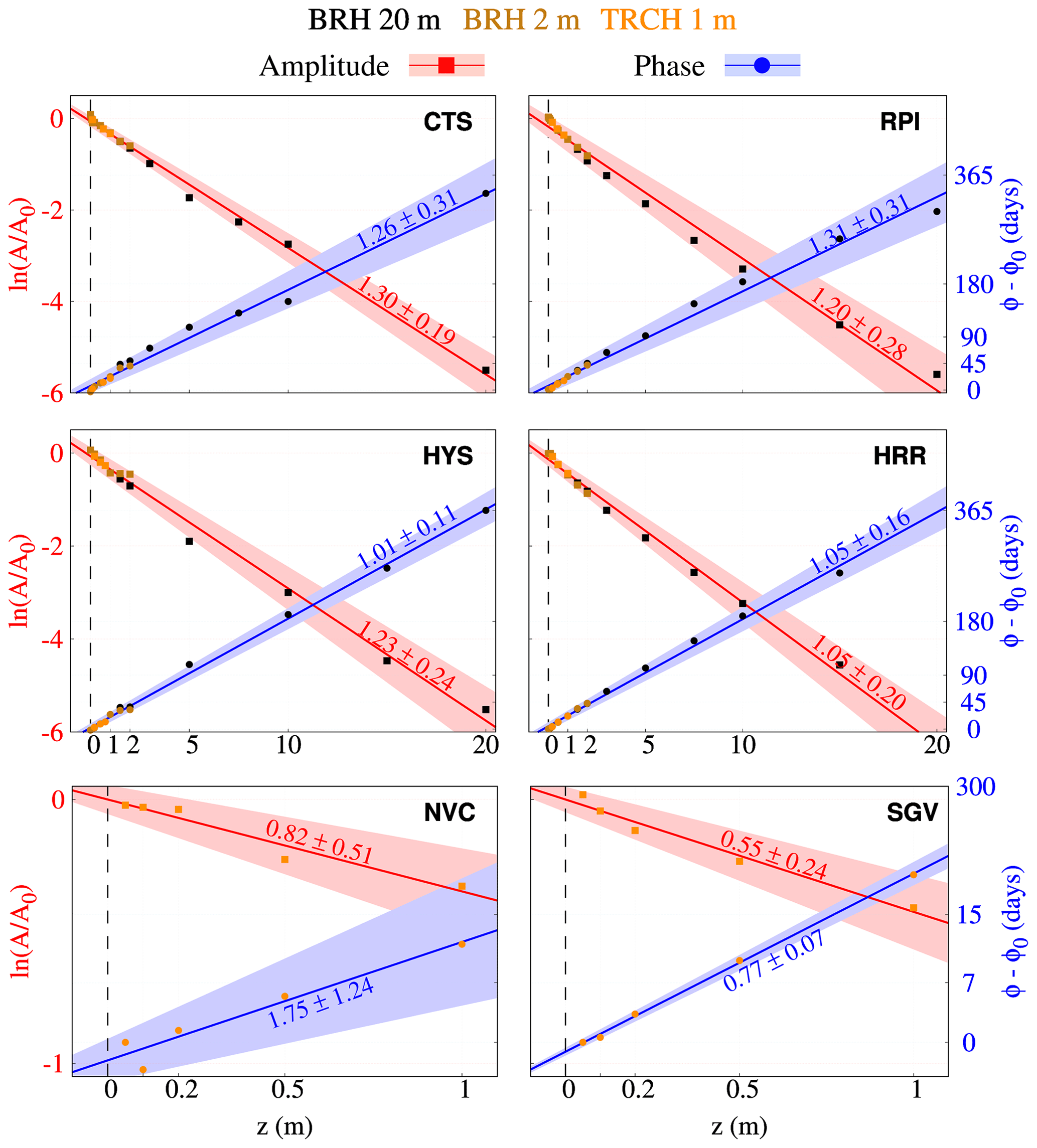
Figure 7Phase shift in days (blue) and the logarithm of amplitude ratios (red) vs. depth at CTS, HYS, RPI, HRR, NVC, and SGV (see Table 1). Points in orange, brown, and black stem from a least-squares adjustment for sinusoidal fitting of the annual cycle of TRCH 1 m, BRH 2 m, and BRH 20 m data, respectively. Diffusivity values (10−6 m2 s−1) are retrieved by linearly fitting all the points available at every site (see the text for details). Regression lines, confidence intervals using a significance level of p=0.05, and diffusivity values for the logarithm of the amplitude ratios (phase shift) are included in red (blue).
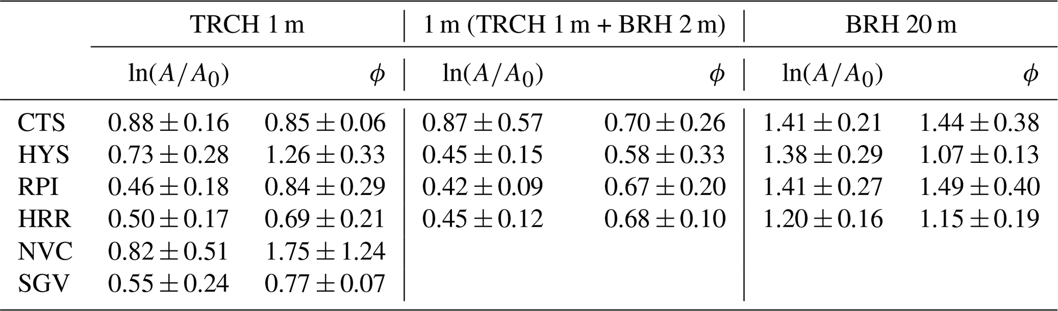
Table 5Apparent thermal diffusivity values (10−6 m2 s−1) obtained from the amplitude attenuation, ln(), and phase shift, ϕ, for TRCH 1 m only (first column), the first meter of depth using a blend of TRCH 1 m and BRH 2 m data (second column), and BRH 20 m (third column) at CTS, HYS, RPI, HRR, SGV, and NVC.
4.2 Subsurface thermal regime: the CA
The subsurface thermal structure in the area of the Sierra de Guadarrama is assessed hereafter. The conductive propagation of GST changes is first addressed by applying a CA (Sect. 3). Results for a CA over the whole profile for every site are included in Fig. 7. As can be seen, CTS, HYS, RPI, and HRR integrate data coming from both BRH 2 m, BRH 20 m, and TRCH 1 m down to 20 m, while NVC and SGV provide TRCH 1 m data. Hence, apparent thermal diffusivity values only account for the first meter underground at these two sites. For the rest of the sites, all the information at each location down to 20 m is used to derive apparent thermal diffusivity estimates. Table 5 segregates results for the case in which only TRCH 1 m would be considered as well as for the cases that include information available down to 1 m (TRCH 1 m + BRH 2 m) and down to 20 m using only BRH 20 m. This information complements the estimates provided in Fig. 7.
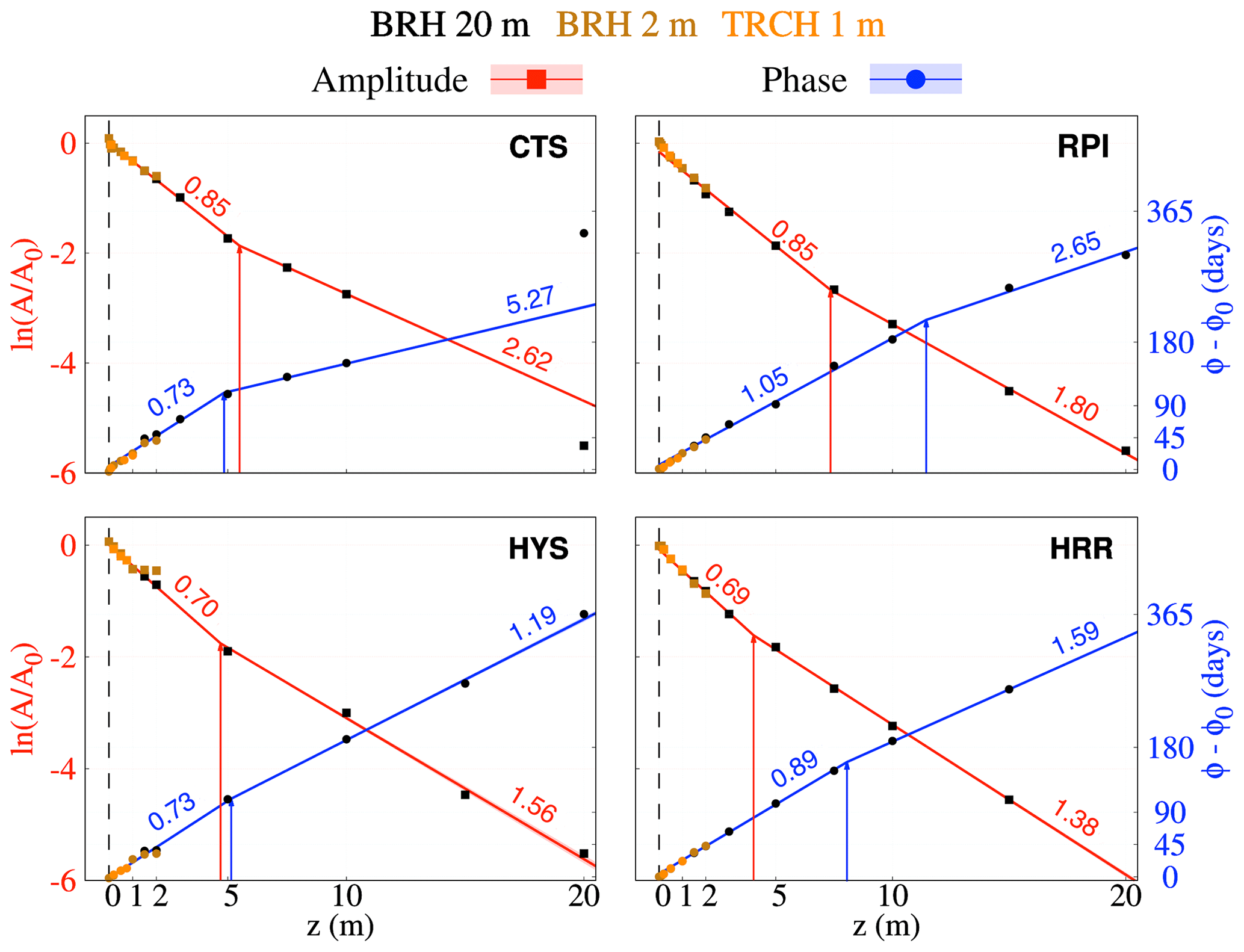
Figure 8Two-phase regression of the points shown in Fig. 7. Lines represent the linear trends that are the best fit to the data before and after the estimated point of change for the logarithm of the amplitude ratio (phase shift), depicted in red (blue). Apparent thermal diffusivity values (10−6 m2 s−1) before and after the change point are given as well in every case. The 20 m level at CTS was omitted from the analysis.
Thermal diffusivity estimates, i.e., apparent thermal diffusivities, yielded from the slope of the regression lines for both phase shift and amplitude attenuation are very similar for all the deep sites, generally in the range of 1– m2 s−1. These values are close to the mineral diffusivity values for quartz (ca. m2 s−1) and feldspar (ca. m2 s−1), two of the main components of gneiss and granite (de Vries, 1963), which are the dominating materials found at the sites of this study (Fig. 2). The observations at SGV render values that fall below this range, with apparent diffusivity values between 0.5 and m2 s−1. While subsurface temperatures at CTS, HYS, RPI, and HRR extensively cover the soil and bedrock depths, NVC and SGV only include data within the first meter of the soil, which can yield very different thermal diffusivity estimates with respect to the other sites. Near the surface, the different composition, compactness, and soil moisture content can account for the different apparent diffusivity values. In fact, if apparent diffusivity is estimated at all the sites using only TRCH 1 m observations, values in the range of 0.46 (RPI) to m2 s−1 (CTS) are attained (Table 5). Furthermore, if both TRCH 1 m and BRH 2 m temperatures within the first meter are considered, values hardly change and range from 0.42 (RPI) to m2 s−1 (CTS). It is often the case that apparent diffusivity values rendered by amplitude attenuation and phase shift within the first meter of the soil can differ considerably, as shown for NVC in Fig. 7. This is an indication that changes in apparent thermal diffusivity occur towards the surface, as seen at NVC and SGV in Fig. 7. Additionally, changes in the conductive regime may occur within these depths due to soil moisture variability (Melo-Aguilar et al., 2022), freezing and thawing processes (Gao et al., 2008), and near-surface evaporation and latent heat exchanges (Tong et al., 2017) affecting the soil.
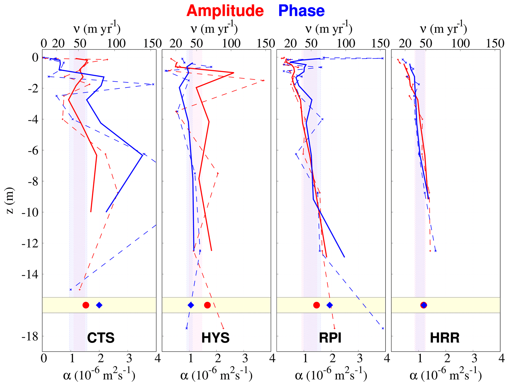
Figure 9Thermal diffusivity (α, 10−6 m2 s−1) and wave velocity (ν, m yr−1) profiles with depth (m). The red curves were obtained from normalized amplitude attenuation values ln() and the blue ones from phase-shift values with depth. Dashed (solid) lines represent the raw (three-running-layer thickness-weighted average) estimate. Points at the bottom of the profile (shaded yellow) represent the thickness-weighted average of the whole subsurface profile. Shaded areas in red (blue) represent the thermal diffusivity values obtained by linearly fitting the amplitude attenuation (phase shift) in Fig. 7.
The regression spread when considering deep sites in Fig. 7 can be remarkable, scaling up to 25 % at RPI. Even if the logarithm of the amplitude damping and phase shift for the whole soil column can be considered linear in a first approach, values do not seem to distribute randomly around the regression line. For instance, between 2 and 7 m all the sites tend to show larger-amplitude attenuations and phase shifts, hence indicating changes in the regression line slope, i.e., diffusivity, with depth. A further analysis using a two-phase regression model (Fig. 8; Solow, 1987, 1995) confirms there is a tilt in the slope, indicating a significant change in the apparent thermal diffusivity values with depth. Even though the coefficient of determination is very high and significant for every site for both the simple CA (Fig. 7) and two-phase CA (Fig. 8) regression lines, always above 0.9, there is a significant reduction in the square sum of residuals in the second case. For instance, this quantity plunges from 5.67 to 1.02 at HYS and from 8.22 to 0.62 at RPI for amplitude attenuation and from 3.21 to 0.91 and from 11.46 to 1.20 d2 for phase shift, respectively, thus indicating that the two-phase regression represents the data more accurately than a single-slope linear regression model. Since amplitude attenuation and phase-shift values at every depth were normalized before applying the CA (see Sect. 3), the change point position is certainly not produced by gathering information from TRCH 1 m and the BRHs. A change in apparent thermal diffusivity might be indicative of the soil–bedrock transition, where porous non-consolidated material is progressively substituted by consolidated and more compacted material, which yields higher diffusivity values with depth (de Vries, 1963; Pollack et al., 2005). Apparent diffusivity values scale up from 0.7–1 to 1.4– m2 s−1 at most of the sites, which is consistent with the aforementioned transition. In Fig. 8, CTS and HYS show similar change point values for the amplitude attenuation and the phase shift analysis around 5 m. However, there is more uncertainty at RPI and HRR, where amplitude attenuation yields shallower change points (7 and 4 m) than the phase shift analysis (11 and 8 m, respectively).
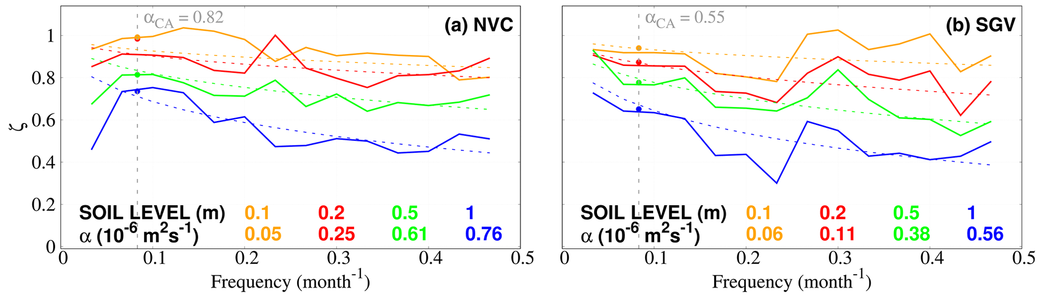
Figure 10SpM amplitude attenuation analysis at NVC (a) and SGV (b). Monthly time series at both sites were selected for a common interval spanning from 1999 to 2008. Missing data were linearly interpolated. Spectral attenuation curves are calculated as a ratio of amplitudes of Welch's periodogram at the (Stoica and Moses, 1997) 0.1 (orange), 0.2 (red), 0.5 (green), and 1 (blue) m temperature levels with respect to GST. Solid (dashed) lines represent observed (theoretical) curves at every level. Diffusivity values below come from least-squares fitting the observed to theoretical curves. Diffusivity values in grey (top left of each panel) show the result of the CA for the amplitude attenuation of the annual cycle ( month−1) shown in Fig. 7. Colored points at the annual frequency (vertical grey dashed line) show the corresponding result of the CA for the amplitude attenuation at every level with respect to GST, which can be compared with the corresponding SpM observed (solid) and theoretical (dashed) values.
The previous changes in apparent diffusivity inferred by the CA can be partially traced to the soil–bedrock transitions observed in Fig. 2 (see Sect. 2), where the profiles of subsurface composition have a superficial soil layer which is succeeded by accumulated sediments and crystalline materials of granite and gneiss. Results coming from the CA and the stratigraphy of the samples agree at HYS, placing the soil–bedrock transition at a depth of 5 m. However, if the change points should be due to the bedrock limit, the CA underestimates the observed depth at CTS, where the bedrock starts in the sampled cores at 8 m (Fig. 8). The fact that the amplitude attenuation and phase shift CA results do not coincide at RPI and HRR might also be an indication that other factors influence the occurrence of change points (e.g., soil moisture), the CA failing again to produce consistent amplitude and phase estimates for change points, both above the values of sampled cores that show the soil–bedrock transition at 5 and 2 m, respectively. Considering the combined results from the stratigraphy and the CA for the four sites, it becomes clear that there is some uncertainty in the relationship between subsurface material and apparent thermal diffusivity changes, and other influences play a role in producing the step changes in thermal properties with depth.
The aforementioned sample analysis illustrates that changes in subsurface material do not occur abruptly but rather progressively into depth, contributing to changes in apparent thermal diffusivity with depth as well. For that reason, subsurface diffusivity profiles were derived by applying the CA level by level to CTS, HYS, RPI, and HRR (Fig. 9). This shows that diffusivity increases with depth at every site, which agrees with a previous analysis conducted at Fargo (Smerdon et al., 2003). Whilst RPI and HRR manifest a more linear behavior, apparent thermal diffusivity values at CTS and HYS differ considerably from one layer to the other, with the profiles being particularly variable near the surface. In general, the mean diffusivity values and spread attained in Fig. 7 are well represented by the profiles, being higher at the deepest layers. Since diffusivity estimates in Fig. 9 are weighted by the layer thickness, small values in the thinner soil layers near the surface are down-weighted and the total vertical estimates tend to be greater than those provided in Fig. 7. Overall, Fig. 9 agrees well with results derived from Figs. 2, 7, and 8 and Table 5 and illustrates better the deviations from the linear behavior for the natural logarithm of amplitude attenuation and the phase shift with depth identified in Fig. 7. These deviations are explained by an increase in apparent thermal diffusivity with depth.
4.3 Subsurface thermal regime: the SpM
Heterogeneity near the surface and soil moisture spatial and temporal variability can produce changes in diffusivity. To study this effect, the SpM is introduced in the analysis, taking into account the damping of all temperature perturbation amplitudes in the frequency spectrum but overlooking alterations of the conductive regime due to convection, advection, or latent heat exchange processes (Gao et al., 2008; Tong et al., 2017). Nevertheless, it can provide some hints of the diffusivity changes with depth and mostly with time. An example of its performance is given in Fig. 10, where it was applied to monthly temperature data at SGV and NVC in the 1999–2008 period. Apparent thermal diffusivity was retrieved at the 0.05, 0.1, 0.25, and 0.5 m layers assessing the spectral amplitude attenuation of GST in its propagation to the 0.1, 0.2, 0.5, and 1 m levels, respectively. Results for both sites show that soil thermal diffusivity increases with depth, being higher for NVC than for SGV. The value of the apparent thermal diffusivity for the whole soil column derived from the SpM at SGV (see the points in Fig. 10) agrees with the CA estimate at the annual frequency from Fig. 7 ( month−1; 0.55 for CA vs. m2 s−1 for the SpM), while it is slightly smaller at NVC (0.82 vs. m2 s−1). The consistency of the CA and SpM in reproducing the amplitude attenuation of the annual cycle indicates the robustness of the SpM in reproducing CA results. Furthermore, the SpM allows for extension of the amplitude attenuation analysis to the whole harmonic spectrum. This means that shorter periods, i.e., higher frequencies than the annual cycle, can be considered. In fact, the application of the SpM is not limited to data at monthly resolution but is applicable to higher temporal resolutions.
Figure 11 expands the use of the SpM as an example to estimate thermal diffusivity values for weekly (a), 3-daily (b), daily (c), and 3-hourly (d) resolutions at HRR. One can observe how the SpM consistently reproduces the amplitude attenuation of the annual cycle stemming from CA at every resolution. Moreover, Fig. 11 shows the effect of frequency in amplitude decay: whilst in Fig. 11a the observed amplitude attenuation curves show an exponential decay in every case, with values over except for 1 m, all the levels in Fig. 11d are affected by poor signal-to-noise ratios at the high frequencies. Therefore, filtering out unreliable amplitude attenuation values at high frequencies with a suitable criterion (e2-fold decay in our case) becomes crucial for preventing biased thermal diffusivity estimates. If the whole frequency band was considered in the SpM, unbiased estimates would still be attained at shallow soil layers and low frequencies, but poor performance should be expected at the deep and high ones, respectively.
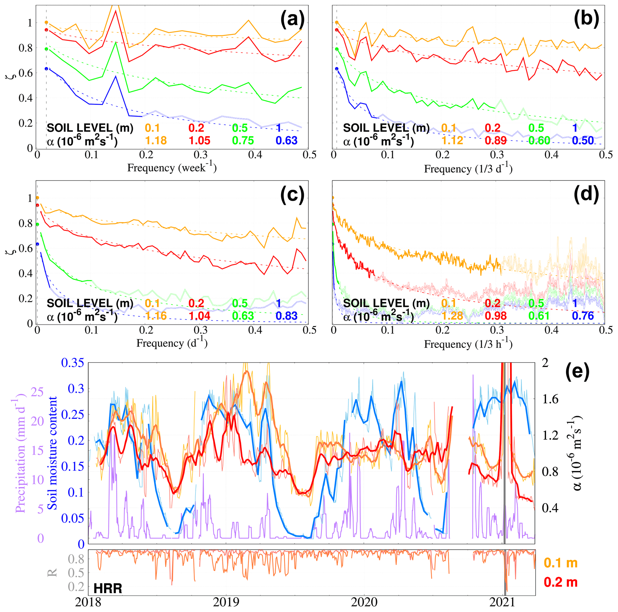
Figure 11As in Fig. 10, SpM analysis of subsurface temperature attenuation at HRR for weekly (a), 3-daily (b), daily (c), and 3-hourly (d) data. The hollow parts of the observed attenuation curves were excluded in the estimation of apparent thermal diffusivity according to the e2-fold decay criterion explained in Sect. 3. (e) Precipitation, soil moisture content, and estimated near-surface thermal diffusivity from applying the SpM at the 0.1 m (light orange) and 0.2 m (light red) levels with respect to the GST with a 10 d running window at 3-hourly resolution; 11 d low-pass running averages are provided in dark colors. Soil moisture content at 4 cm is shown at daily (10-daily) resolution in light blue (blue). Precipitation at 10-daily resolution is shown in purple. The least-square regression correlation (R) for SpM at every time step is given below in each case. The grey-shaded thick line represents the only time interval (4 d) with snow insulation in Fig. 6c for HRR.
As has already been mentioned, soil properties are especially heterogeneous near the surface due to interactive changes in soil material, texture (Cermak et al., 2017), moisture, and hydrology (Pollack et al., 2005; Gao et al., 2008; Tong et al., 2017). The last factor mostly affects subsurface thermal conductivity and volumetric heat capacity by filling up the empty pore spaces embedded in the soil (Arkhangelskaya and Lukyashchenko, 2018), which in turn modifies the apparent thermal diffusivity. Figure 11e explores the relation between soil moisture content and apparent thermal diffusivity near the surface at HRR.
The SpM at 3-hourly resolution (Fig. 11e) in a 10 d running window is applied to derive an intra-monthly evolution of apparent thermal diffusivity at the shallowest layers (0.1 and 0.2 m), which is subsequently compared to changes in soil moisture and precipitation. It is observed that soil moisture presents a seasonal cycle, with extremely low content values in summer and relatively high but variable values in winter and spring. Transitions between these two states are remarkably abrupt, with soil moisture content increasing substantially by the beginning of fall and responding to enhanced precipitation and with the opposite occurring by the end of spring. In contrast to the other sites in the Sierra de Guadarrama, HRR is rarely snow-covered in winter, which usually occurs after high-impact snow events (e.g., Filomena, which hit the Iberian Peninsula in January 2021; shading in Figs. 6c and 11e; Smart, 2021; Tapiador et al., 2021). Apparent thermal diffusivity also shows a seasonal behavior, which corresponds to soil moisture low-frequency variability. In summer, poor soil moisture content drives apparent thermal diffusivity values down. However, even though diffusivity in winter increases with soil moisture content, the relation between these two variables at the high frequencies is not conclusive. For instance, the evolution of diffusivity in winter–spring 2018 at both soil levels correctly mimics soil moisture content variations (Fig. 11e) yet fails to capture its strong variations in winter 2020. This agrees with a clear increase in apparent thermal diffusivity from dry to wet soils but a rather stable diffusivity in wet soils close to its field capacity observed by Arkhangelskaya and Lukyashchenko (2018). An analogous result for thermal conductivity by Dai et al. (2019) complies with this result as well. Moreover, SpM fails to provide reliable estimates of apparent thermal diffusivity when the ground is insulated by the snow, due to signal loss in the whole frequency band. This is clearly shown in Fig. 11e in January 2021, when the R coefficient, i.e., the square root of the goodness of fit of the amplitude attenuation to an exponential function, becomes extremely poor.
Interannual correlation is hard to establish from our assessment due to the shortness of the time series in Fig. 11. However, previous studies (e.g., Melo-Aguilar et al., 2022) suggest that soil moisture and apparent thermal diffusivity changes are proportionally related to some degree. Nevertheless, the lack of strong evidence of a linear relationship between apparent thermal diffusivity and soil moisture near the surface could also suggest that heat conduction is no longer the most important mechanism of heat transfer. Heat convective transport via soil moisture and latent energy fluxes, water advection, and horizontal heat transport due to uneven temperature changes at the ground surface can also contribute to modifying the vertical heat conduction regime near the surface. The use of a running-window SpM over longer time series or developing an alternate SpM based on a conductive–convective amplitude attenuation (Gao et al., 2008; Tong et al., 2017) solution to the heat diffusion equation might better define this relation in wet soils.
The subsurface thermal structure at six sites in the Sierra de Guadarrama is consistent with the hypothesis of conduction being the main heat propagation mechanism of SAT changes into depth. On the one hand, SAT changes are transferred to the near surface at the ground. Although SAT and GST are coupled at long timescales, snow insulation and zero-curtain effects produce a decoupling in winter at the uppermost stations (CTS, HYS, and RPI), which are affected by the presence of a seasonal snow cap (Figs. 5 and 6). This result agrees with previous studies carried out at cold and snowy sites, such as Fargo (North Dakota, US; Smerdon et al., 2003), Emigrant Pass (Utah, US; Bartlett et al., 2006), Bistriţa (Romania; Demetrescu et al., 2007), and Hveravellir (Iceland; Petersen, 2022).
On the other hand, GST changes are propagated to depth by heat conduction to an extent controlled by the apparent thermal diffusivity of the subsurface. A CA method based on the amplitude attenuation and phase shift of the annual cycle yielded values that are between 1 and m2 s−1 for the whole soil column (i.e., 20 m) at most of the sites (Fig. 7), which are in the range of typical diffusivity values for granite or gneiss, the main materials found in the Sierra de Guadarrama's subsurface (Fig. 2). These values are higher than those observed at the other sites (e.g., Fargo, Prague, or Cape Henlopen; Smerdon et al., 2004), which include shallower measures. If apparent thermal diffusivity is assessed near the surface, the values are smaller than and closer to the previous literature (0.4 to m2 s−1; Table 5). A subsequent two-phase adjustment (Fig. 8) and a profile derivation based on CA (Fig. 9) portray an increase in thermal diffusivity with depth at all the sites, being more remarkable near the soil–bedrock transition. Evaluating thermal diffusivity changes with depth using a CA can therefore be a useful approach to determine soil depth at observational sites when no borehole rock samples are available. The deep monitoring profiles at the Sierra de Guadarrama are unique and provide a wider insight into subsurface thermal structure, which may have implications for calibrating soil and bedrock properties in models (Tong et al., 2016; Dai et al., 2019) and monitoring land heat uptake in the terrestrial energy budget (Cuesta-Valero et al., 2022, 2023; von Schuckmann et al., 2023).
Near-surface (i.e., 1 m) soil apparent thermal diffusivity vertical and temporal heterogeneity is further explored by introducing a new SpM, which extends the analysis of temperature amplitude attenuation to the whole frequency spectrum. The SpM reports consistent apparent thermal diffusivity values in the first soil meter at SGV, NVC, and HRR with those previously derived with the CA for each of the respective sites regardless of the time resolution of the input data. Then, it was used in an intra-monthly (10-daily) sliding window to explore apparent thermal diffusivity changes in time at the ground surface at HRR (Fig. 11e). Results suggest that this parameter presents a seasonal cycle that is positively correlated with soil moisture, mostly under soil drought conditions. However, the fact that these changes are poorly correlated under high soil moisture contents might indicate that heat conduction is not the main heat transfer mechanism in wet soils. Heat transport via water advection and phase changes might not be negligible near the surface, so the thermal structure in the shallow soil could be better characterized using a modification of the SpM that complies with a conduction–convection heat transfer equation (Gao et al., 2008; Tong et al., 2017). Even so, the results show the potential of the SpM for inferring soil moisture content changes from soil temperatures, becoming a powerful tool for evaluating soil drought and water resource availability from observational and simulation-based subsurface temperature data.
Quality-controlled temperature data at daily resolution and the most relevant codes for data processing used in this work are available at Zenodo (https://doi.org/10.5281/zenodo.7499419, García-Pereira et al., 2023). Nevertheless, all data can be freely obtained for research from the original data sources, GuMNet and AEMET (see Sect. 2 for the web addresses). Further details of the code are available upon request to the corresponding author.
FGP and JFGR conceptualized and drafted the manuscript. TS, JFGR, and CVC collected the data. FGP processed the data and developed the methodologies. CVC and CMA contributed to data processing. NJS, PRG, FJCV, AGG, HB, and PdV revised the manuscript and contributed to the writing and discussion. JFGR supervised this work.
The contact author has declared that none of the authors has any competing interests.
Publisher’s note: Copernicus Publications remains neutral with regard to jurisdictional claims made in the text, published maps, institutional affiliations, or any other geographical representation in this paper. While Copernicus Publications makes every effort to include appropriate place names, the final responsibility lies with the authors.
This work has been developed through the Spanish Council of Research (CSIC) in the frame of the Interdisciplinary Thematic Platform (PTI) Polar zone observatory (PTI POLARCSIC). We are also thankful for the data provided by the GuMNet (https://www.ucm.es/gumnet/, last access: 29 December 2022) and AEMET (https://www.aemet.es/en/datos_abiertos/, last access: 29 December 2022) meteorological networks.
This research has been supported by the SMILEME (contract no. PID2021-126696OBC21) project, funded by MCIN/AEI/10.13039/501100011033 from the Spanish Ministry of Science and Innovation (MICINN). Félix García-Pereira was funded by contract no. PRE2019-090694 of the MICINN. Cristina Vegas-Cañas was funded by contract no. PTA2020-019839-I. Francisco José Cuesta-Valero was funded by the Alexander von Humboldt Foundation.
We acknowledge the support of the publication fee by the CSIC Open Access Publication Support Initiative through its Unit of Information Resources for Research (URICI).
This paper was edited by Paul Hallett and reviewed by two anonymous referees.
Abbott, B. W. and Jones, J. B.: Permafrost collapse alters soil carbon stocks, respiration, CH4, and N2O in upland tundra, Global Change Biol., 21, 4570–4587, https://doi.org/10.1111/gcb.13069, 2015. a
Andresen, C. G., Lawrence, D. M., Wilson, C. J., McGuire, A. D., Koven, C., Schaefer, K., Jafarov, E., Peng, S., Chen, X., Gouttevin, I., Burke, E., Chadburn, S., Ji, D., Chen, G., Hayes, D., and Zhang, W.: Soil moisture and hydrology projections of the permafrost region – a model intercomparison, The Cryosphere, 14, 445–459, https://doi.org/10.5194/tc-14-445-2020, 2020. a
Arkhangelskaya, T. and Lukyashchenko, K.: Estimating soil thermal diffusivity at different water contents from easily available data on soil texture, bulk density, and organic carbon content, Biosyst. Eng., 168, 83–95, https://doi.org/10.1016/j.biosystemseng.2017.06.011, 2018. a, b
Bartlett, M. G., Chapman, D. S., and Harris, R. N.: Snow effect on North American ground temperatures, 1950–2002, J. Geophys. Res.-Earth, 110, F03008, https://doi.org/10.1029/2005JF000293, 2005. a, b
Bartlett, M. G., Chapman, D. S., and Harris, R. N.: A Decade of Ground–Air Temperature Tracking at Emigrant Pass Observatory, Utah, J. Climate, 19, 3722–3731, https://doi.org/10.1175/JCLI3808.1, 2006. a, b, c
Beltrami, H. and Kellman, L.: An examination of short- and long-term air–ground temperature coupling, Global Planet. Change, 38, 291–303, https://doi.org/10.1016/S0921-8181(03)00112-7, 2003. a, b, c
Beltrami, H., Smerdon, J. E., Pollack, H. N., and Huang, S.: Continental heat gain in the global climate system, Geophys. Res. Lett., 29, 8-1–8-3, https://doi.org/10.1029/2001GL014310, 2002. a
Bond-Lamberty, B. and Thomson, A.: Temperature-Associated Increases in the Global Soil Respiration Record, Nature, 464, 579–82, https://doi.org/10.1038/nature08930, 2010. a
Brady, N. C. and Weil, R. R.: The nature and properties of soils, 15th edition, Pearson Prentice Hall, Upper Saddle River, NJ, United States, ISBN 0133254488, 2017. a, b
Brandsma, T. and Können, G. P.: Application of nearest-neighbor resampling for homogenizing temperature records on a daily to sub-daily level, Int. J. Climatol., 26, 75–89, https://doi.org/10.1002/joc.1236, 2006. a
Brigham, E. O. and Morrow, R. E.: The fast Fourier transform, IEEE Spec., 4, 63–70, https://doi.org/10.1109/MSPEC.1967.5217220, 1967. a
Burke, E. J., Zhang, Y., and Krinner, G.: Evaluating permafrost physics in the Coupled Model Intercomparison Project 6 (CMIP6) models and their sensitivity to climate change, The Cryosphere, 14, 3155–3174, https://doi.org/10.5194/tc-14-3155-2020, 2020. a
Carslaw, H. S. and Jaeger, J. C.: Conduction of heat in solids, Vol. 2 Edn., Clarendon Press, Oxford University Press, Oxford, United Kingdom, ISBN 0198533683, 1959. a, b, c, d
Cermak, V. and Bodri, L.: Attribution of precipitation changes on ground–air temperature offset: Granger causality analysis, Int. J. Earth Sci., 107, 145–152, https://doi.org/10.1007/s00531-016-1351-y, 2016. a, b
Cermak, V., Bodri, L., Šafanda, J., Kresl, M., and Dedecek, P.: Ground-air temperature tracking and multi-year cycles in the subsurface temperature time series at geothermal climate-change observatory, Stud. Geophys. Geod., 58, 403–424, https://doi.org/10.1007/s11200-013-0356-2, 2014. a
Cermak, V., Bodri, L., Kresl, M., Dedecek, P., and Safanda, J.: Eleven years of ground–air temperature tracking over different land cover types, Int. J. Climatol., 37, 1084–1099, https://doi.org/10.1002/joc.4764, 2017. a, b
Chen, D., Rojas, M., Samset, B., Cobb, K., Niang, A. D., Edwards, P., Emori, S., Faria, S., E. Hawkins, P. H., Huybrechts, P., Meinshausen, M., Mustafa, S., Plattner, G.-K., and Tréguier, A.-M.: Introduction, in: Climate Change 2021: The Physical Science Basis, Contribution of Working Group I to the Sixth Assessment Report of the Intergovernmental Panel on Climate Change, edited by: Masson-Delmotte, V., Zhai, P., Pirani, A., Connors, S. L., Péan, C., Berger, S., Caud, N., Chen, Y., Goldfarb, L., Gomis, M. I., Huang, M., Leitzell, K., Lonnoy, E., Matthews, J. B. R., Maycock, T. K., Waterfield, T., Yelekçi, O., Yu, R., and Zhou, B., Cambridge University Press, Cambridge, 147–286, https://doi.org/10.1017/9781009157896.003, 2021. a, b, c
Cuesta-Valero, F. J., Beltrami, H., Gruber, S., García-García, A., and González-Rouco, J. F.: A new bootstrap technique to quantify uncertainty in estimates of ground surface temperature and ground heat flux histories from geothermal data, Geosci. Model Dev., 15, 7913–7932, https://doi.org/10.5194/gmd-15-7913-2022, 2022. a, b
Cuesta-Valero, F. J., Beltrami, H., García-García, A., Krinner, G., Langer, M., MacDougall, A. H., Nitzbon, J., Peng, J., von Schuckmann, K., Seneviratne, S. I., Thiery, W., Vanderkelen, I., and Wu, T.: Continental heat storage: contributions from the ground, inland waters, and permafrost thawing, Earth Syst. Dynam., 14, 609–627, https://doi.org/10.5194/esd-14-609-2023, 2023. a, b
Dai, Y., Wei, N., Yuan, H., Zhang, S., Shangguan, W., Liu, S., Lu, X., and Xin, Y.: Evaluation of Soil Thermal Conductivity Schemes for Use in Land Surface Modeling, J. Adv. Model. Earth Sy., 11, 3454–3473, https://doi.org/10.1029/2019MS001723, 2019. a, b
de Vrese, P., Georgievski, G., Gonzalez Rouco, J. F., Notz, D., Stacke, T., Steinert, N. J., Wilkenskjeld, S., and Brovkin, V.: Representation of soil hydrology in permafrost regions may explain large part of inter-model spread in simulated Arctic and subarctic climate, The Cryosphere, 17, 2095–2118, https://doi.org/10.5194/tc-17-2095-2023, 2023. a
de Vries, D. A.: Thermal properties of soil, in: Physics of Plant Environment, edited by: van Dijk, W. R., North Holland Publishing, Amsterdam, 210–235, 1963. a, b
Demetrescu, C., Nitoiu, D., Boroneant, C., Marica, A., and Lucaschi, B.: Thermal signal propagation in soils in Romania: conductive and non-conductive processes, Clim. Past, 3, 637–645, https://doi.org/10.5194/cp-3-637-2007, 2007. a, b
Dorau, K., Bamminger, C., Koch, D., and Mansfeldt, T.: Evidences of soil warming from long-term trends (1951–2018) in North Rhine-Westphalia, Germany, Clim. Change, 170, 1–13, https://doi.org/10.1007/s10584-021-03293-, 2022. a
Dědeček, P., Rajver, D., Čermák, V., Šafanda, J., and Krešl, M.: Six years of ground–air temperature tracking at Malence (Slovenia): thermal diffusivity from subsurface temperature data, J. Geophys. Eng., 10, 025012, https://doi.org/10.1088/1742-2132/10/2/025012, 2013. a
Ekici, A., Beer, C., Hagemann, S., Boike, J., Langer, M., and Hauck, C.: Simulating high-latitude permafrost regions by the JSBACH terrestrial ecosystem model, Geosci. Model Dev., 7, 631–647, https://doi.org/10.5194/gmd-7-631-2014, 2014. a
Eyring, V., Bony, S., Meehl, G. A., Senior, C. A., Stevens, B., Stouffer, R. J., and Taylor, K. E.: Overview of the Coupled Model Intercomparison Project Phase 6 (CMIP6) experimental design and organization, Geosci. Model Dev., 9, 1937–1958, https://doi.org/10.5194/gmd-9-1937-2016, 2016. a
Fuchs, S., Förster, H.-J., Norden, B., Balling, N., Miele, R., Heckenbach, E., and Förster, A.: The Thermal Diffusivity of Sedimentary Rocks: Empirical Validation of a Physically Based α−ϕ Relation, J. Geophys. Res.-Sol. Ea., 126, e2020JB020595, https://doi.org/10.1029/2020JB020595, 2021. a
Gao, Z., Lenschow, D. H., Horton, R., Zhou, M., Wang, L., and Wen, J.: Comparison of two soil temperature algorithms for a bare ground site on the Loess Plateau in China, J. Geophys. Res.-Atmos., 113, D18105, https://doi.org/10.1029/2008JD010285, 2008. a, b, c, d, e, f
García-García, A., Cuesta-Valero, F. J., Beltrami, H., and Smerdon, J. E.: Simulation of air and ground temperatures in PMIP3/CMIP5 last millennium simulations: implications for climate reconstructions from borehole temperature profiles, Environ. Res. Lett., 11, 044022, https://doi.org/10.1088/1748-9326/11/4/044022, 2016. a
García-García, A., Cuesta-Valero, F. J., Beltrami, H., and Smerdon, J. E.: Characterization of Air and Ground Temperature Relationships within the CMIP5 Historical and Future Climate Simulations, J. Geophys. Res.-Atmos., 124, 3903–3929, https://doi.org/10.1029/2018JD030117, 2019. a
García-Pereira, F., González-Rouco, J. F., Schmid, T., Melo-Aguilar, C., Vegas-Cañas, C., Steinert, N. J., Roldán-Gómez, P. J., Cuesta-Valero, F. J., García-García, A., Beltrami, H., and de Vrese, P.: Thermodynamic and hydrological drivers of the subsurface thermal regime in Central Spain: open data and code (1.0), Zenodo [data set], https://doi.org/10.5281/zenodo.7499419, 2023. a
González-Rouco, J. F., Beltrami, H., Zorita, E., and von Storch, H.: Simulation and inversion of borehole temperature profiles in surrogate climates: Spatial distribution and surface coupling, Geophys. Res. Lett., 33, L01703, https://doi.org/10.1029/2005GL024693, 2006. a
González-Rouco, J. F., Beltrami, H., Zorita, E., and Stevens, M. B.: Borehole climatology: a discussion based on contributions from climate modeling, Clim. Past, 5, 97–127, https://doi.org/10.5194/cp-5-97-2009, 2009. a
González-Rouco, J. F., Steinert, N. J., García-Bustamante, E., Hagemann, S., de Vrese, P., Jungclaus, J. H., Lorenz, S. J., Melo-Aguilar, C., García-Pereira, F., and Navarro, J.: Increasing the depth of a Land Surface Model. Part I: Impacts on the soil thermal regime and energy storage, J. Hydrometeorol., 22, 3211–3230, https://doi.org/10.1175/JHM-D-21-0024.1, 2021. a
Gulev, S., Thorne, P., Ahn, J., Dentener, F., Domingues, C., Gerland, S., Gong, D., Kaufman, D., Nnamchi, H., Quaas, J., Rivera, J., Sathyendranath, S., Smith, S., Trewin, B., von Schuckmann, K., and Vose, R.: Changing State of the Climate System, in: Climate Change 2021: The Physical Science Basis. Contribution of Working Group I to the Sixth Assessment Report of the Intergovernmental Panel on Climate Change edited by: Masson-Delmotte, V., Zhai, P., Pirani, A., Connors, S. L., Péan, C., Berger, S., Caud, N., Chen, Y., Goldfarb, L., Gomis, M. I., Huang, M., Leitzell, K., Lonnoy, E., Matthews, J. B. R., Maycock, T. K., Waterfield, T., Yelekçi, O., Yu, R., and Zhou, B., Cambridge University Press, Cambridge, 287–422, https://doi.org/10.1017/9781009157896.004, 2021. a
Hansen, J., Ruedy, R., Sato, M., and Lo, K.: Global surface temperature change, Rev. Geophys., 48, RG4004, https://doi.org/10.1029/2010RG000345, 2010. a
Hermoso de Mendoza, I., Beltrami, H., MacDougall, A. H., and Mareschal, J.-C.: Lower boundary conditions in land surface models – effects on the permafrost and the carbon pools: a case study with CLM4.5, Geosci. Model Dev., 13, 1663–1683, https://doi.org/10.5194/gmd-13-1663-2020, 2020. a
Huang, S., Pollack, H., and Shen, P.: Temperature trends over the five past centuries reconstructed from borehole temperature, Nature, 403, 756–758, https://doi.org/10.1038/35001556, 2000. a
Hurley, S. and Wiltshire, R.: Computing thermal diffusivity from soil temperature measurements, Comput. Geosci., 19, 475–477, https://doi.org/10.1016/0098-3004(93)90096-N, 1993. a, b
Jaume-Santero, F., Pickler, C., Beltrami, H., and Mareschal, J.-C.: North American regional climate reconstruction from ground surface temperature histories, Clim. Past, 12, 2181–2194, https://doi.org/10.5194/cp-12-2181-2016, 2016. a
Jones, P. D., Lister, D. H., Osborn, T. J., Harpham, C., Salmon, M., and Morice, C. P.: Hemispheric and large-scale land-surface air temperature variations: An extensive revision and an update to 2010, J. Geophys. Res.-Atmos., 117, D05127, https://doi.org/10.1029/2011JD017139, 2012. a
Krakauer, N. Y., Puma, M. J., and Cook, B. I.: Impacts of soil–aquifer heat and water fluxes on simulated global climate, Hydrol. Earth Syst. Sci., 17, 1963–1974, https://doi.org/10.5194/hess-17-1963-2013, 2013. a
Lawrimore, J. H., Menne, M. J., Gleason, B. E., Williams, C. N., Wuertz, D. B., Vose, R. S., and Rennie, J.: An overview of the Global Historical Climatology Network monthly mean temperature data set, version 3, J. Geophys. Res.-Atmos., 116, D19121, https://doi.org/10.1029/2011JD016187, 2011. a
Lenssen, N. J. L., Schmidt, G. A., Hansen, J. E., Menne, M. J., Persin, A., Ruedy, R., and Zyss, D.: Improvements in the GISTEMP Uncertainty Model, J. Geophys. Res.-Atmos., 124, 6307–6326, https://doi.org/10.1029/2018JD029522, 2019. a
Lesperance, M., Smerdon, J. E., and Beltrami, H.: Propagation of linear surface air temperature trends into the terrestrial subsurface, J. Geophys. Res.-Atmos., 115, D21115, https://doi.org/10.1029/2010JD014377, 2010. a
Maher, N., Milinski, S., Suarez-Gutierrez, L., Botzet, M., Dobrynin, M., Kornblueh, L., Kröger, J., Takano, Y., Ghosh, R., Hedemann, C., Li, C., Li, H., Manzini, E., Notz, D., Putrasahan, D., Boysen, L., Claussen, M., Ilyina, T., Olonscheck, D., Raddatz, T., Stevens, B., and Marotzke, J.: The Max Planck Institute Grand Ensemble: Enabling the Exploration of Climate System Variability, J. Adv. Model. Earth Sy., 11, 2050–2069, https://doi.org/10.1029/2019MS001639, 2019. a
Mareschal, J. and Beltrami, H.: Evidence for recent warming from perturbed geothermal gradients: examples from eastern Canada, Clim. Dynam., 6, 135–143, https://doi.org/10.1007/BF00193525, 1992. a
Melo-Aguilar, C., González-Rouco, J. F., García-Bustamante, E., Navarro-Montesinos, J., and Steinert, N.: Influence of radiative forcing factors on ground–air temperature coupling during the last millennium: implications for borehole climatology, Clim. Past, 14, 1583–1606, https://doi.org/10.5194/cp-14-1583-2018, 2018. a, b, c, d
Melo-Aguilar, C., González-Rouco, F., Steinert, N. J., Beltrami, H., Cuesta-Valero, F. J., García-García, A., García-Pereira, F., García-Bustamante, E., Roldán-Gómez, P. J., Schmid, T., and Navarro, J.: Near-surface soil thermal regime and land–air temperature coupling: a case study over Spain, Int. J. Climatol., 42, 7516–7534, https://doi.org/10.1002/joc.7662, 2022. a, b, c, d, e
Miralles, D. G., Gentine, P., Seneviratne, S. I., and Teuling, A. J.: Land–atmospheric feedbacks during droughts and heatwaves: state of the science and current challenges, Ann. NY Acad. Sci., 1436, 19–35, https://doi.org/10.1111/nyas.13912, 2019. a, b
Osborn, T. J., Jones, P. D., Lister, D. H., Morice, C. P., Simpson, I. R., Winn, J. P., Hogan, E., and Harris, I. C.: Land Surface Air Temperature Variations Across the Globe Updated to 2019: The CRUTEM5 Data Set, J. Geophys. Res.-Atmos., 126, e2019JD032352, https://doi.org/10.1029/2019JD032352, 2021. a
Outcalt, S. I., Nelson, F. E., and Hinkel, K. M.: The zero-curtain effect: Heat and mass transfer across an isothermal region in freezing soil, Water Resour. Res., 26, 1509–1516, https://doi.org/10.1029/WR026i007p01509, 1990. a
Pegoraro, E. F., Mauritz, M. E., Ogle, K., Ebert, C. H., and Schuur, E. A. G.: Lower soil moisture and deep soil temperatures in thermokarst features increase old soil carbon loss after 10 years of experimental permafrost warming, Global Change Biol., 27, 1293–1308, https://doi.org/10.1111/gcb.15481, 2021. a
Petersen, G. N.: Trends in soil temperature in the Icelandic highlands from 1977 to 2019, Int. J. Climatol., 42, 2299–2310, https://doi.org/10.1002/joc.7366, 2022. a, b
Pollack, H. N. and Huang, S.: Climate Reconstruction from Subsurface Temperatures, Annu. Rev. Earth Pl. Sc., 28, 339–365, https://doi.org/10.1146/annurev.earth.28.1.339, 2000. a
Pollack, H. N. and Smerdon, J. E.: Borehole climate reconstructions: Spatial structure and hemispheric averages, J. Geophys. Res.-Atmos., 109, D11106, https://doi.org/10.1029/2003JD004163, 2004. a
Pollack, H. N., Smerdon, J. E., and van Keken, P. E.: Variable seasonal coupling between air and ground temperatures: A simple representation in terms of subsurface thermal diffusivity, Geophys. Res. Lett., 32, L15405, https://doi.org/10.1029/2005GL023869, 2005. a, b, c
Pries, C. E. H., Castanha, C., Porras, R. C., and Torn, M. S.: The whole-soil carbon flux in response to warming, Science, 355, 1420–1423, https://doi.org/10.1126/science.aal1319, 2017. a, b
Putnam, S. N. and Chapman, D. S.: A geothermal climate change observatory: First year results from Emigrant Pass in northwest Utah, J. Geophys. Res.-Sol. Ea., 101, 21877–21890, https://doi.org/10.1029/96JB01903, 1996. a, b
Rohde, R., Muller, R. A., Jacobsen, R., Muller, E., Perlmutter, S., Rosenfeld, A., Wurtele, J., Groom, D., and Wickham, C.: A New Estimate of the Average Earth Surface Land Temperature Spanning 1753 to 2011, Geoinfo. Geostat., 1, 1–7, https://doi.org/10.4172/2327-4581.1000101, 2013. a
Rotta Loria, A.: The silent impact of underground climate change on civil infrastructure, Commun. Eng., 2, 44, https://doi.org/10.1038/s44172-023-00092-1, 2023. a
Schaefer, K., Elshorbany, Y., Jafarov, E., Schuster, P., Striegl, R., Wickland, K., and Sunderland, E.: Potential impacts of mercury released from thawing permafrost, Nat. Commun., 11, 4650, https://doi.org/10.1038/s41467-020-18398-5, 2020. a
Schlesinger, W. H. and Emily, S. B.: Biogeochemistry: an analysis of global change, 3 Edn., Academic Press, Amsterdam, Netherlands, ISBN 0123858747, 2013. a
Seneviratne, S., Zhang, X., Adnan, M., Badi, W., Dereczynski, C., Luca, A. D., Ghosh, S., Iskandar, I., Kossin, J., Lewis, S., Otto, F., Pinto, I., Satoh, M., Vicente-Serrano, S., Wehner, M., and Zhou, B.: Weather and Climate Extreme Events in a Changing Climate, in: Climate Change 2021: The Physical Science Basis, Contribution of Working Group I to the Sixth Assessment Report of the Intergovernmental Panel on Climate Change, edited by: Masson-Delmotte, V., Zhai, P., Pirani, A., Connors, S. L., Péan, C., Berger, S., Caud, N., Chen, Y., Goldfarb, L., Gomis, M. I., Huang, M., Leitzell, K., Lonnoy, E., Matthews, J. B. R., Maycock, T. K., Waterfield, T., Yelekçi, O., Yu, R., and Zhou, B., Cambridge University Press, Cambridge, 1513–1766, https://doi.org/10.1017/9781009157896.013, 2021. a
Smart, D.: Storm Filomena 8 January 2021, Weather, 76, 98–99, https://doi.org/10.1002/wea.3950, 2021. a
Smerdon, J. E. and Stieglitz, M.: Simulating heat transport of harmonic temperature signals in the Earth's shallow subsurface: Lower-boundary sensitivities, Geophys. Res. Lett., 33, L14402, https://doi.org/10.1029/2006GL026816, 2006. a, b
Smerdon, J. E., Pollack, H. N., Enz, J. W., and Lewis, M. J.: Conduction-dominated heat transport of the annual temperature signal in soil, J. Geophys. Res.-Sol. Ea., 108, 2431, https://doi.org/10.1029/2002JB002351, 2003. a, b, c
Smerdon, J. E., Pollack, H. N., Cermak, V., Enz, J. W., Kresl, M., Safanda, J., and Wehmiller, J. F.: Air-ground temperature coupling and subsurface propagation of annual temperature signals, J. Geophys. Res.-Atmos., 109, D21107, https://doi.org/10.1029/2004JD005056, 2004. a, b, c, d, e, f
Smerdon, J. E., Pollack, H. N., Cermak, V., Enz, J. W., Kresl, M., Safanda, J., and Wehmiller, J. F.: Daily, seasonal, and annual relationships between air and subsurface temperatures, J. Geophys. Res.-Atmos., 111, D07101, https://doi.org/10.1029/2004JD005578, 2006. a
Smerdon, J. E., Beltrami, H., Creelman, C., and Stevens, M. B.: Characterizing land surface processes: A quantitative analysis using air-ground thermal orbits, J. Geophys. Res.-Atmos., 114, D15102, https://doi.org/10.1029/2009JD011768, 2009. a, b
Solow, A. R.: Testing for Climate Change: An Application of the Two-Phase Regression Model, J. Appl. Meteorol. Clim., 26, 1401–1405, https://doi.org/10.1175/1520-0450(1987)026<1401:TFCCAA>2.0.CO;2, 1987. a, b
Solow, A. R.: Testing for Change in the Frequency of El Niño Events, J. Climate, 8, 2563–2566, https://doi.org/10.1175/1520-0442(1995)008<2563:TFCITF>2.0.CO;2, 1995. a, b
Soong, J. L., Castanha, C., Pries, C. E. H., Ofiti, N., Porras, R. C., Riley, W. J., Schmidt, M. W., and Torn, M. S.: Five years of whole-soil warming led to loss of subsoil carbon stocks and increased CO2 efflux, Sci. Adv., 7, eabd1343, https://doi.org/10.1126/sciadv.abd1343, 2021. a
Sorour, M., Saleh, M., and Mahmoud, R.: Thermal conductivity and diffusivity of soil, Int. Comm. Heat Mass Transf., 17, 189–199, https://doi.org/10.1016/0735-1933(90)90053-M, 1990. a
Steinert, N. J., González-Rouco, J. F., de Vrese, P., García-Bustamante, E., Hagemann, S., Melo-Aguilar, C., Jungclaus, J. H., and Lorenz, S. J.: Increasing the depth of a Land Surface Model. Part II: Sensitivity to improved coupling between soil hydrology and thermodynamics and associated permafrost response, J. Hydrometeorol., 22, 3231–3254, https://doi.org/10.1175/JHM-D-21-0023.1, 2021. a
Stoica, P. and Moses, R.: Introduction to spectral analysis, Prentice Hall, Upper Saddle River, N.J., United States, ISBN 0132584190, 1997. a, b
Tapiador, F. J., Villalba-Pradas, A., Navarro, A., Martín, R., Merino, A., García-Ortega, E., Sánchez, J. L., Kim, K., and Lee, G.: A Satellite View of an Intense Snowfall in Madrid (Spain): The Storm “Filomena” in January 2021, Remote Sens., 13, 2702, https://doi.org/10.3390/rs13142702, 2021. a
Taylor, K. E., Stouffer, R. J., and Meehl, G. A.: An Overview of CMIP5 and the Experiment Design, B. Am. Meteorol. Soc., 93, 485–498, https://doi.org/10.1175/BAMS-D-11-00094.1, 2012. a
Tong, B., Gao, Z., Horton, R., Li, Y., and Wang, L.: An Empirical Model for Estimating Soil Thermal Conductivity from Soil Water Content and Porosity, J. Hydrometeorol., 17, 601–613, https://doi.org/10.1175/JHM-D-15-0119.1, 2016. a
Tong, B., Gao, Z., Horton, R., and Wang, L.: Soil Apparent Thermal Diffusivity Estimated by Conduction and by Conduction–Convection Heat Transfer Models, J. Hydrometeorol., 18, 109–118, https://doi.org/10.1175/JHM-D-16-0086.1, 2017. a, b, c, d, e, f
Tukey, J. W.: Exploratory Data Analysis, Addison-Wesley Publishing Company Reading, Massachusetts, https://doi.org/10.1002/bimj.4710230408, 1977. a
Turetsky, M., Abbott, B., Jones, M., Walter Anthony, K., Olefeldt, D., Schuur, E., Koven, C., McGuire, A., Grosse, G., Kuhry, P., Hugelius, G., Lawrence, D., Gibson, C., and Sannel, A.: Permafrost collapse is accelerating carbon release, Nature, 569, 32–34, https://doi.org/10.1038/d41586-019-01313-4, 2019. a
Vegas-Cañas, C., González-Rouco, J. F., Navarro-Montesinos, J., García-Bustamante, E., Lucio-Eceiza, E. E., García-Pereira, F., Rodríguez-Camino, E., Chazarra-Bernabé, A., and Álvarez Arévalo, I.: An Assessment of Observed and Simulated Temperature Variability in Sierra de Guadarrama, Atmosphere, 11, 985, https://doi.org/10.3390/atmos11090985, 2020. a, b, c, d
Vicente-Serrano, S., Azorin-Molina, C., Sanchez-Lorenzo, A., Morán-Tejeda, E., Lorenzo-Lacruz, J., Revuelto, J., López-Moreno, J., and Espejo, F.: Temporal evolution of surface humidity in Spain: Recent trends and possible physical mechanisms, Clim. Dynam., 42, 2655–2674, https://doi.org/10.1007/s00382-013-1885-7, 2013. a
von Schuckmann, K., Minière, A., Gues, F., Cuesta-Valero, F. J., Kirchengast, G., Adusumilli, S., Straneo, F., Ablain, M., Allan, R. P., Barker, P. M., Beltrami, H., Blazquez, A., Boyer, T., Cheng, L., Church, J., Desbruyeres, D., Dolman, H., Domingues, C. M., García-García, A., Giglio, D., Gilson, J. E., Gorfer, M., Haimberger, L., Hakuba, M. Z., Hendricks, S., Hosoda, S., Johnson, G. C., Killick, R., King, B., Kolodziejczyk, N., Korosov, A., Krinner, G., Kuusela, M., Landerer, F. W., Langer, M., Lavergne, T., Lawrence, I., Li, Y., Lyman, J., Marti, F., Marzeion, B., Mayer, M., MacDougall, A. H., McDougall, T., Monselesan, D. P., Nitzbon, J., Otosaka, I., Peng, J., Purkey, S., Roemmich, D., Sato, K., Sato, K., Savita, A., Schweiger, A., Shepherd, A., Seneviratne, S. I., Simons, L., Slater, D. A., Slater, T., Steiner, A. K., Suga, T., Szekely, T., Thiery, W., Timmermans, M.-L., Vanderkelen, I., Wjiffels, S. E., Wu, T., and Zemp, M.: Heat stored in the Earth system 1960–2020: where does the energy go?, Earth Syst. Sci. Data, 15, 1675–1709, https://doi.org/10.5194/essd-15-1675-2023, 2023. a, b
von Storch, H.: Climate models and modeling: an editorial essay, WIREs Clim. Change, 1, 305–310, https://doi.org/10.1002/wcc.12, 2010. a
Zhang, T.: Influence of the seasonal snow cover on the ground thermal regime: An overview, Rev. Geophys., 43, RG4002, https://doi.org/10.1029/2004RG000157, 2005. a
Zhou, S., Williams, A., Berg, A., Cook, B., Zhang, Y., Hagemann, S., Lorenz, R., Seneviratne, S., and Gentine, P.: Land–atmosphere feedbacks exacerbate concurrent soil drought and atmospheric aridity, P. Natl. Acad. Sci. USA, 116, 18848–18853, https://doi.org/10.1073/pnas.1904955116, 2019. a