SoilGrids 2.0: producing soil information for the globe with quantified spatial uncertainty

SoilGrids produces maps of soil properties for the entire globe at medium spatial resolution (250 m cell size) using state-of-the-art machine learning methods to generate the necessary models. It takes as inputs soil observations from about 240 000 locations worldwide and over 400 global environmental covariates describing vegetation, terrain morphology, climate, geology and hydrology. The aim of this work was the production of global maps of soil properties, with cross-validation, hyper-parameter selection and quantification of spatially explicit uncertainty, as implemented in the SoilGrids version 2.0 product incorporating state-of-the-art practices and adapting them for global digital soil mapping with legacy data. The paper presents the evaluation of the global predictions produced for soil organic carbon content, total nitrogen, coarse fragments, pH (water), cation exchange capacity, bulk density and texture fractions at six standard depths (up to 200 cm). The quantitative evaluation showed metrics in line with previous global, continental and large-region studies. The qualitative evaluation showed that coarse-scale patterns are well reproduced. The spatial uncertainty at global scale highlighted the need for more soil observations, especially in high-latitude regions.

1 Introduction

Healthy soils provide important ecosystem services at the local, landscape and global level and are important for the functioning of terrestrial ecosystems (Banwart et al., 2014; FAO and ITPS, 2015; UNEP, 2012). Information on world soil resources, based on the currently “best available” (shared) soil profile data, at a scale level commensurate with user needs, is required to address a range of pressing global issues. These include avoiding and reducing soil erosion through land rehabilitation and development (Borrelli et al., 2017; WOCAT, 2007), mitigating and adapting to climate change (Batjes, 2019; Harden et al., 2017; Sanderman et al., 2017; Yigini and Panagos, 2016; Smith et al., 2019) and ensuring water security (Rockstroem et al., 2012), food production and food security (FAO et al., 2018; Soussana et al., 2017; Springmann et al., 2018), as well as preserving biodiversity (Barnes, 2015; IPBES, 2019; van der Esch et al., 2017) and human livelihood (Bouma, 2015).

The best available soil data are required to support the Land Degradation Neutrality (LDN) (Cowie et al., 2018) initiative, achieve several of the Sustainable Development Goals and provide input for, for example, Earth system modelling by the IPCC (Dai et al., 2019; Luo et al., 2016; Todd-Brown et al., 2013) and crop modelling (Han et al., 2019; van Bussel et al., 2015; van Ittersum et al., 2013), among many other applications. Such information can in turn help inform international conventions such as the United Nations Framework Convention on Climate Change (UNFCCC), the United Nation Convention to Combat Desertification (UNCCD) and the United Nations Convention on Biological Diversity (UNCBD).

Until the last decade, most global scale assessments requiring soil data used the Digital Soil Map of the World (DSMW) FAO (1995), an updated version of the original printed 1:5 ×10⁶ scale Soil Map of the World (SMW) (FAO-Unesco, 1971–1981). The soil geographic data from the DSMW provided the basis for generating a range of derived soil property databases that drew on a larger selection of soil profile data held in the WISE database (Batjes, 2012) and more sophisticated (taxotransfer) procedures for deriving various soil properties (Batjes et al., 2007). Subsequently, in a joint effort coordinated by the Food and Agriculture Organization of the United Nations (FAO), the best available (newer) soil information collated for central and southern Africa, China, Europe, northern Eurasia and Latin America was combined into a new product known as the Harmonised World Soil Database (HWSD) (FAO et al., 2012).

Until recently, the HWSD was the only digital map annex database available for global analyses. However, it has several limitations (GSP and FAO, 2016; Hengl et al., 2014; Ivushkin et al., 2019; Omuto et al., 2012). Some of these relate to the partly outdated soil geographic data, as well as the use of a two-layer model (0–30 and 30–100 cm) for deriving soil properties. Others concern the derived attribute data themselves, in particular their unquantified uncertainty, and the use of three different versions of the FAO legend (i.e. FAO74, FAO85 and FAO90). These issues have been addressed to varying degrees in various new global soil datasets (Batjes, 2016; Shangguan et al., 2014; Stoorvogel et al., 2017) that still largely draw on a traditional soil mapping approach (Dai et al., 2019).

In the last decade, digital soil mapping (DSM) has become a widely used approach to obtain maps of soil information (Minasny and McBratney, 2016). DSM consists primarily in building a quantitative numerical model between soil observations and environmental information acting as proxies for the soil forming factors (McBratney et al., 2003; Minasny and McBratney, 2016). DSM can also integrate direct information as proxies for soil properties, for example proximal sensing measurements. The number of studies using DSM to produce maps of soil properties is ever growing. Numerous modelling approaches are considered, from linear models to geostatistics, machine learning and artificial intelligence (e.g. deep learning). Keskin and Grunwald (2018) provide a recent review of methods and applications in the field of DSM. DSM techniques have been applied at various spatial resolutions (e.g. 30 to 1000 m) to support precision farming (e.g. Piikki et al., 2017) as well as applications at landscape (e.g. Ellili et al., 2019; Kempen et al., 2015), country (e.g. Mora-Vallejo et al., 2008; Nijbroek et al., 2018; Vitharana et al., 2019; Poggio and Gimona, 2017b; Kempen et al., 2019), regional (e.g. Dorji et al., 2014; Moulatlet et al., 2017), continental (e.g. Grunwald et al., 2011; Guevara et al., 2018; Hengl et al., 2017a) and global levels (e.g. Hengl et al., 2014, 2017b; GSP and ITPS, 2018; Stockmann et al., 2015).

The aim of this paper is to present the development of new soil property maps for the world at 250 m grid resolution with a process incorporating state-of-the-art practices and adapting them to the challenges of global digital soil mapping with legacy data. It builds on previous global soil properties maps (SoilGrids250m) (Hengl et al., 2017b), integrating up-to-date machine learning methods, the increased availability of standardised soil profile data for the world (Batjes et al., 2020) and environmental covariates (Nussbaum et al., 2018; Poggio et al., 2013; Reuter and Hengl, 2012). In particular, this paper addresses the following elements at global scale:

1. incorporation of soil profile data derived from ISRIC's World Soil Information Service (WoSIS), with expanded number and spatial distribution of observations (Batjes et al., 2020);

2. a reproducible covariate selection procedure, relying on recursive feature elimination (Guyon et al., 2002);

3. improved cross-validation procedure, based on spatial stratification; and

4. quantification of prediction uncertainty using quantile regression forests (Meinshausen, 2006).

2 Materials and methods

This study uses quantile regression forests (Meinshausen, 2006), a method with a limited number of parameters to be tuned and that has proven to be an effective compromise between accuracy and feasibility for large datasets. Selected primary soil properties as defined and described in the GlobalSoilMap specifications (Arrouays et al., 2014) were modelled. The following sections describe each step of the workflow (Fig. 1) in detail. These include the following:

1. input soil data preparation

2. covariates' selection

3. model tuning and cross-validation

4. final model fitting for prediction

5. predictions with uncertainty estimation.

Figure 1 Workflow of the methodological approach.

Table 1 Soil properties description and units.

^∗ unitless.

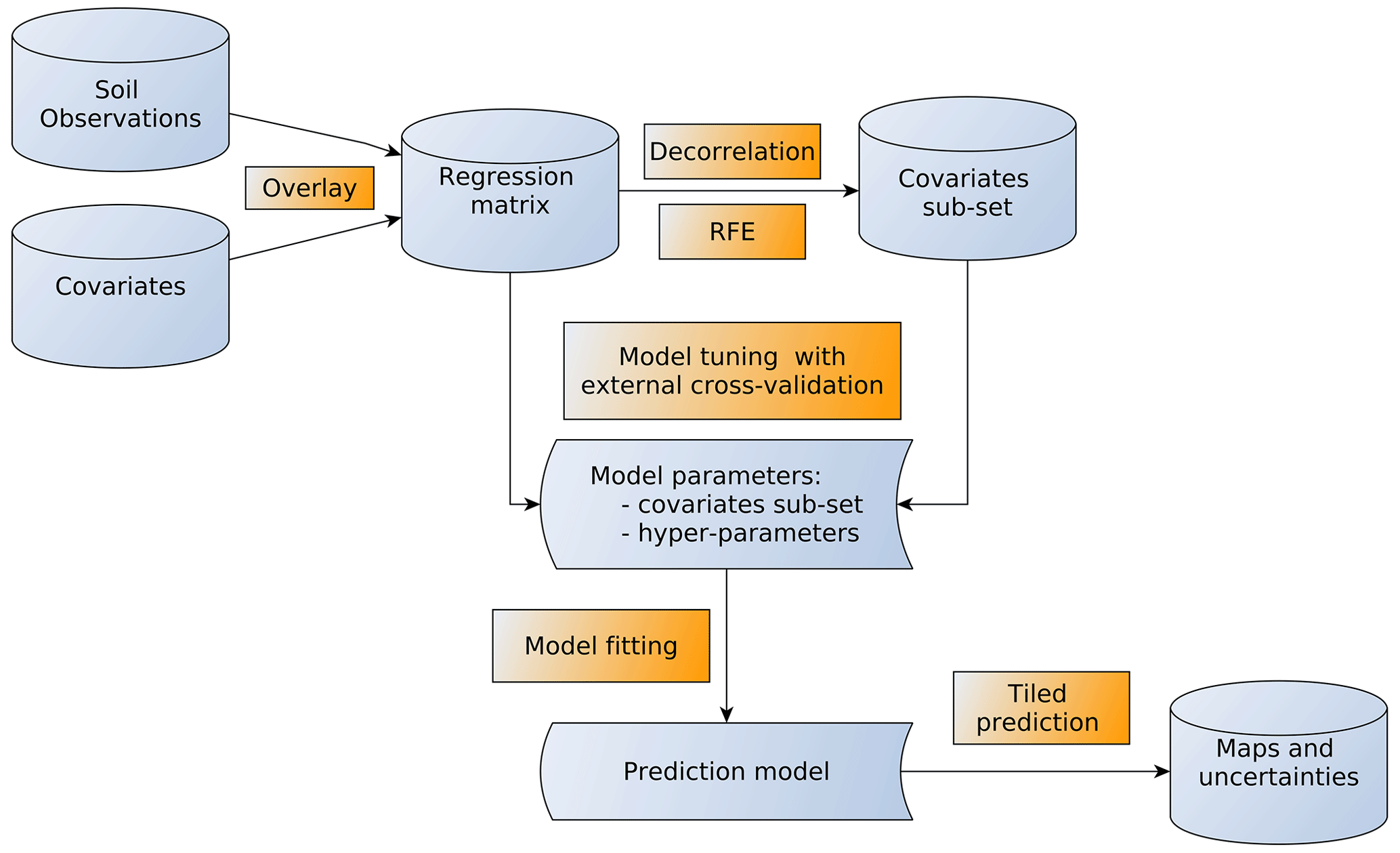
2.1 Soil observation data

Soil property data for this study were derived from the ISRIC World Soil Information Service (WoSIS), which provides consistent, standardised soil profile data for the world (Batjes et al., 2020). All soil data shared with ISRIC to support global mapping activities are first stored in the ISRIC Data Repository, together with their metadata (including the name of the data owner and licence defining access rights). Subsequently, the source data are imported “as is” into PostgreSQL, after which they are ingested into the WoSIS data model itself. Following data quality assessment and control (including consistency checks on latitude–longitude and depth of horizon/layer; flagging of duplicate profiles; and providing measures for geographic and attribute accuracy, as well as time stamps), the descriptions for the soil analytical methods and the units of measurement are standardised using consistent procedures, with additional checks for possible erroneous entries for the soil analytical data themselves (Ribeiro et al., 2018). Ultimately, upon final consistency checks, the standardised data are made available via the ISRIC Soil Data Hub (https://data.isric.org, last access: 20 May 2021) in accord with the licence specified by the data providers. As a result, not all data standardised in WoSIS are freely available to the international community. Hence, this study considers two “sources” of point data.

The first is the latest publicly available snapshot of WoSIS (Batjes et al., 2020). It contains, among others, data for chemical (organic carbon, total nitrogen, soil pH, cation exchange capacity) and physical properties (soil texture (sand, silt and clay), coarse fragments). The snapshot comprises 196 498 georeferenced profiles originating from 173 countries, representing over 832 000 soil layers (or horizons), in total over 5.8 million records. Generally, there are more observations for the superficial than the deeper layers. About 5 % of the profiles were sampled before 1960, 14 % between 1961–1980, 32 % between 1981–2000 and 16 % between 2001–2020; the date of sampling is unknown for 34 % of the shared profiles (Batjes et al., 2020).

Second, in addition to the freely shareable data, several soil observation databases in our repository have licences stipulating that ISRIC may only use them for SoilGrids applications or visualisations, for example EU-LUCAS (Tóth et al., 2013) and soil data for the state of Victoria (Australia). The corresponding source datasets were screened and processed using the same procedures as used for the regular WoSIS workflow (some 42 000 profiles). As a result, some 240 000 profiles in total were used as the data source for the present 2020 SoilGrids run, comprising more than 920 000 observed soil layers. During data processing some minor corrections were made to the merged input dataset, for example further depth congruence checks.

2.1.1 Soil properties

For the purposes of SoilGrids, “soil” is up to 2 m thick unconsolidated material at the Earth's epidermis in direct contact with the atmosphere; thus subaqueous and tidally exposed soils are not considered here. Neither are materials deeper than 2 m. This decision has consequences for computations of total stocks, in particular soil organic carbon.

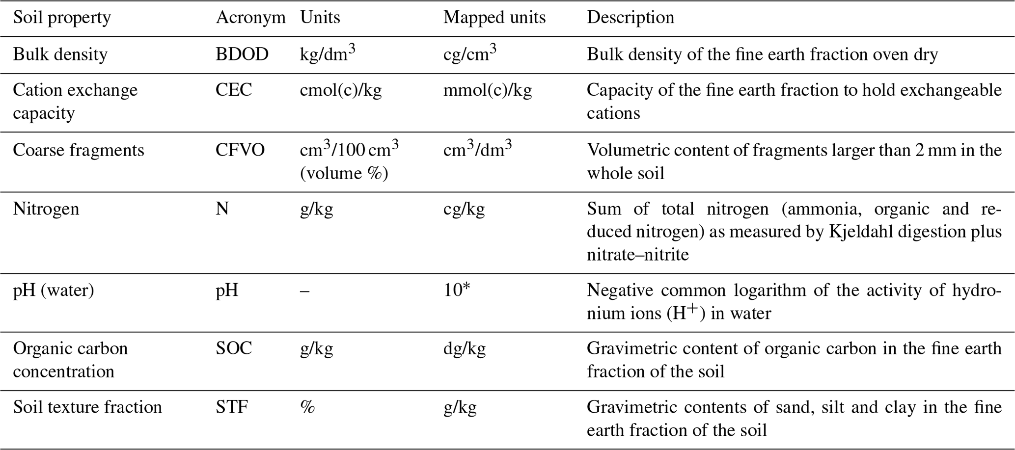
Table 1 describes the soil properties that are considered in this version of SoilGrids: organic carbon content, total nitrogen content, soil pH (measured in water), cation exchange capacity, soil texture fractions and proportion of coarse fragments. These properties were modelled for the six standard depths intervals as defined in the GlobalSoilMap specifications (Arrouays et al., 2014): 0–5, 5–15, 15–30, 30–60, 60–100 and 100–200 cm.

“Litter layers” on top of minerals soils were excluded from further modelling using the following assumptions. Consistency in layer depth (e.g. sequential increase in the upper and lower depth reported for each layer down the profile) in WoSIS was checked using automated procedures. In accord with current internationally accepted conventions, such depth increments are given as “measured from the surface, including organic layers and mineral covers” (FAO, 2006; Schoeneberger et al., 2012). Prior to 1993, however, the start (zero depth) of the profile was set at the top of the mineral surface (the solum proper), except when “thick” organic layers as defined for peat soils (FAO-ISRIC, 1986) were present at the surface. Then the top of the peat layer was taken as the soil surface. Organic horizons were recorded as above and mineral horizons recorded as below, relative to the mineral surface (Schoeneberger et al., 2012) (p. 2–6). Insofar as is possible, “superficial litter” on top of mineral layers was flagged as an auxiliary (Boolean) variable, also with reference to the original soil horizon designation when provided, so it can be filtered out during auxiliary computations of soil properties.

2.1.2 Transformation of texture data

A transformation was applied to the texture fractions, as follows. The relative percentage of sand, silt and clay can be treated as compositional variables, as the sum of the components always equals 100 %. Therefore, these components were transformed using the addictive log ratio (ALR) transformation with the Gauss–Hermite quadrature (Aitchison, 1986). ALR has previously been applied to soil texture data (Lark and Bishop, 2007; Akpa et al., 2014; Ballabio et al., 2016; Poggio and Gimona, 2017a), and it has been shown (Lark and Bishop, 2007) that ALR-transformed variables preserve information on the spatial correlation and maintain the compositional integrity of the original components. In this study, clay was used as the denominator variable. Therefore the two ALR components that were interpolated can be defined as

$$\begin{array}{}\text{(1)}& \begin{array}{rl}\text{ALR1}& =\log \left({\displaystyle \frac{\text{sand}}{\text{clay}}}\right)\\ \text{ALR2}& =\log \left({\displaystyle \frac{\text{silt}}{\text{clay}}}\right)\end{array}.\end{array}$$

2.1.3 Spatial stratification of observations

Random splitting of profile observations into n cross-validation folds is not suitable in this context, considering the high spatial variation in observation density as it would provide biased results (Brus, 2014). For regions like Europe and North America there are over four profiles per 10 km², whereas for large countries in Asia, such as Kazakhstan, India or Mongolia, the number of available profiles is still quite limited (< one profile per 100 km²) (see Batjes et al., 2020 for further details).

Therefore, soil observations were spatially stratified in the geodetic domain to guarantee a balanced spatial distribution within each cross-validation fold. Spatial strata, in the form of hexagons, were created with an Icosahedral Snyder Equal-Area Grid (ISEAG) of aperture 3 and resolution 6, resulting in 7292 strata (i.e. hexagonal cells), each with an area around 70 000 km². This ISEAG was generated with the dggridR package for the R language (Barnes et al., 2016).

The profiles were assigned to 1 of 10 folds, each equally represented in each stratum, i.e. each cell of the grid previously described. All observations (layers or horizons) belonging to a profile were always in the same fold for both model calibration and evaluation. The caret R package was used to subdivide the locations in the folds while maintaining the spatial distribution.

2.2 Environmental covariates

Over 400 geographic layers were available as environmental covariates for this work. These were chosen for their presumed relation to the major soil forming factors, including long-term soil conditions, i.e. the “time” factor. Appendix A provides a list of the products used as covariates and their sources. The layers considered can be grouped as follows.

• Climate: temperature, precipitation, snowfall, cloud cover, solar radiation, wind speed;

• ecology: bioclimatic zones and ecophysiographic regions;

• geology: soil and sedimentary thickness, rock types;

• land use and cover: from sources such as the European Space Agency (ESA) and U.S. Geological Survey (USGS);

• elevation and terrain morphology: including numerous morphology indexes and landform classes;

• vegetation indexes: such as the normalised difference vegetation index (NDVI), enhanced vegetation index (EVI) and net primary production (NPP);

• raw bands from Landsat and MODIS products;

• hydrography: global water table, inundation and glacier extent, and surface water change.

The average and standard deviation of climatic variables and vegetation indices over 15 years (2001–2015) were computed from monthly data to capture their seasonal dynamics.

All covariates were projected to a common coordinate reference system (CRS), i.e. Goode's homolosine projection for land masses applied to the WGS84 datum. This projection was selected since among the equal-area projections supported by open-source software it is the most effective minimising distortions over land (de Sousa et al., 2019). The projected covariates were imported to GRASS GIS in a normalised raster structure with cells of 250 m by 250 m. Covariates, and hence mapped areas, were restricted to land areas without built-up, water and glacier areas using a mask created from the ESA Land Cover layer for 2015 (Buchhorn et al., 2020). Thus properties of urban and subaqueous soils are not considered.

2.3 Covariates' selection

Considering the large number of available environmental layers, a standardised and reproducible procedure to select covariates used for modelling was implemented to (i) reduce redundancy between covariates, (ii) obtain a more parsimonious and computationally efficient model, (iii) decrease the risk of over-fitting (Gomes et al., 2019) and (iv) avoid a biased assessment of variable importance (Strobl et al., 2008).

The covariates' selection procedure consisted of two steps, de-correlation and recursive feature elimination.

2.3.1 De-correlation analysis

De-correlation analysis was carried out as an initial step to reduce the redundancy of information from more than 400 environmental layers. Only covariate layers that had a pairwise correlation coefficient $<=\mathrm{0.85}$ with all other covariates were included in the subsequent analyses. For each pair of covariates correlated above this threshold, only the first one in alphabetical order was selected for inclusion in the modelling phase. This step reduced the number of initial covariates to approximately 150 layers.

2.3.2 Recursive feature elimination

Recursive feature elimination (RFE) (Guyon et al., 2002) is a methodology that has proven effective to select an optimal set of covariates for regression trees models (Gomes et al., 2019; Hounkpatin et al., 2018). In this study, the RFE procedure implemented in the caret package for the R language (Kuhn, 2015) was used, as it offers a good compromise between accuracy and computation time. The algorithm starts by fitting a model using all covariates, assessing its performance and ranking covariate importance. The least important covariates are then removed from the pool, and again the model is fitted and assessed and the least important covariates removed. The procedure is repeated down to a pool between 0 and n covariates. This procedure is based on out-of-bag (OOB) cross-validation and does not test all covariates' combinations, but it is considered one of the most robust covariates' selection approaches for models like random forests (Nussbaum et al., 2018).

The RFE procedure on the full set of observations and covariates would prove computationally prohibitive. To improve computational feasibility for large datasets, additional steps were developed. Four sets of observations were used for RFE, each obtained using three cross-validation folds (see Sect. 2.1.3 for further details): set 1 contained folds 1 to 3, set 2 folds 4 to 6, set 3 folds 7 to 9 and set 4 contained fold 10 and two other random selected folds. In a first step, the RFE procedure from caret was run independently on each set with default model hyper-parameters for the random forests algorithm as implemented in the ranger package (i.e. ntree as 500 and mtry as the rounded square root of the number variables). In each set, the optimal number and combination of covariates were automatically selected when the model performances stopped increasing, i.e. when the loss function reached its minimum. In this study, the loss function was the OOB root-mean-square error (RMSE).

In the second step, the RFE procedure was applied with all observations and all covariates selected in at least one of the four sets used in the previous step. The final covariate set was the set minimising the loss function.

2.4 Hyper-parameter selection and cross-validation

Figure 2 summarises the approach used for the selection of the model hyper-parameters and the cross-validation. Further details are provided in the following sections.

Figure 2 Detailed workflow for the Hyper-parameter selection and cross-validation.

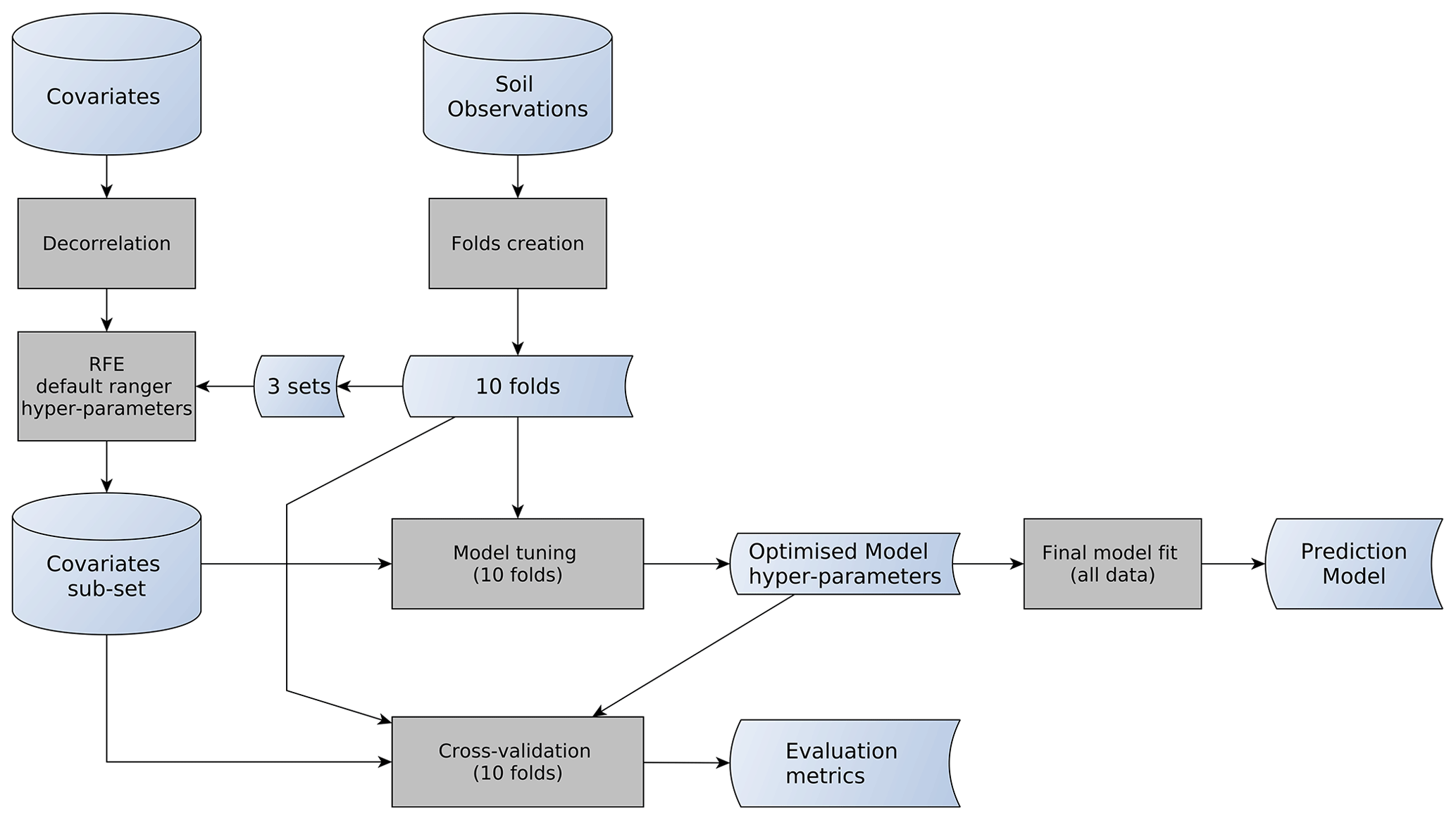
2.4.1 Model tuning and numeric evaluation

Model tuning was performed with a 10-fold cross-validation procedure applied to multiple combinations of hyper-parameters.

Different numbers of decision trees (ntree parameter) were combined with different numbers of covariates used in tree splits (mtry parameter). The number of trees was progressively increased with the following values: 100, 150, 200, 250, 500, 750 and 1000. The different mtry values were multiples of the square root of the number of covariates. Four multipliers were tested, 1 (default in ranger), 1.5, 2 and 3. For example, if the RFE procedure identified a set of 50 covariates, the mtry values assessed were 7, 11, 14 and 21.

Each of the resulting combinations of ntree and mtry parameters was used to train a different model with observations from nine folds. Predictions were then assessed on the remaining fold with classical performance measures, i.e. root mean squared error (RMSE) and model efficiency coefficient (MEC;  Janssen and Heuberger, 1995). MEC is equal to the fraction of the explained variance based on the 1:1 line of predicted versus observed that is defined as 1 minus the ratio between residual sum of squares and total sum of squares. The final hyper-parameter selection was based on an optimisation of model performance and computational constraints, in this case memory consumption. For example an increase of the ntree parameter above 200 provided a minor increment in the metrics (usually less than 0.1 %, not reported here) while requiring considerably more memory and computation time.

The model evaluation was based on the performance metrics of the selected hyper-parameters' combination. Predictions at the centre of the six standard depth intervals were compared with observations having the midpoint included within the considered interval.

2.5 Prediction and uncertainty quantification

2.5.1 Model fit

The final model for each soil property was fitted with all available observations, the covariates and the hyperparameters selected in the previous steps. Observation depth was included in the model as a covariate. It was calculated at the midpoint of the sampled layer or horizon.

Models were obtained with the ranger package (Wright and Ziegler, 2017), with the option quantreg to build quantile random forests (QRF; Meinshausen, 2006). With this option, the prediction is not a single value, e.g. the average of predictions from the group of decision trees in the random forest, but rather a cumulative probability distribution of the soil property at each location and depth.

For each property (see Table 1) and standard depth from the GlobalSoilMap specification (0–5, 5–15, 15–30, 30–60, 60–100 and 100–200 cm), four different values were computed to characterise this distribution: median (0.50 quantile, q_0.50), mean, 0.05 quantile (q_0.05) and 0.95 quantile (q_0.95), i.e. the lower and upper limits of a 90 % prediction interval. This uncertainty interval is as described in the GlobalSoilMap specifications (Arrouays et al., 2014). The predictions were computed for the mid-point of the depth interval and considered constant for the whole depth interval.

In order to compute the prediction uncertainty for soil texture, the back-transformation was applied at the level of individual tree predictions and the quantiles of the tree prediction distributions obtained from the resulting values.

2.5.2 Uncertainty

The percentage of cross-validation observations contained in the 0.9 prediction interval was calculated (prediction interval coverage probability, PICP) (Shrestha and Solomatine, 2006). Ideally the PICP is close to 0.9, indicating that the uncertainty was correctly assessed. A PICP substantially greater than 0.9 suggests that the uncertainty was underestimated; a substantially smaller PICP indicates that it was overestimated.

Furthermore, to visualise the uncertainty as a map, the following indicators were calculated:

1. 90th prediction interval (PI90)

   $$\begin{array}{}\text{(2)}& \text{PI90}=q_{\mathrm{0.95}}-q_{\mathrm{0.05}};\end{array}$$

2. ratio of the interquartile range over the median (prediction interval ratio, PIR):

   $$\begin{array}{}\text{(3)}& \text{PIR}={\displaystyle \frac{q_{\mathrm{0.95}}-q_{\mathrm{0.05}}}{q_{\mathrm{0.50}}}}.\end{array}$$

2.6 Qualitative evaluation of spatial patterns

Expert judgement was used to evaluate the reasonableness of the maps, by comparing well-known spatial patterns at global, regional and local scales with SoilGrids predictions (see Sect. 3.4). Obviously these are not definitive evaluations, only indicative.

2.7 Software and computational framework

SoilGrids requires an intensive computational workflow, with numerous steps integrating different software. SoilGrids is entirely based on open-source software, in particular SLURM (Yoo et al., 2003) for job management, GRASS GIS (GRASS Development Team, 2020) for data and tiles' management and R statistical software (R Core Team, 2020) for model fitting and statistical analysis.

Predictions were computed in a high-performance computing cluster. A dynamic geographic tiling system was developed with GRASS GIS to maximise the use of memory for each job. Technical details on this parallelisation scheme are given in de Sousa et al. (2020).

The predictions were multiplied by a conversion factor of 10 or 100 to maintain the required precision while using integer type in the file geotiff to reduce space occupied on disk. Application of the conversion factor resulted in mapped layers with units differing from those of the input observations (see Table 1).

The total computation time with the selected covariates and hyper-parameters differed per property. On average, the complete computation of the 24 maps (mean and three quantiles for each of the six standard depths) for a single property, including (i) RFE, (ii) model training and (iii) prediction, took approximately 1500 CPU hours. The prediction accounted for about two-thirds of the total time.

3 Results and discussion

3.1 Input soil observations

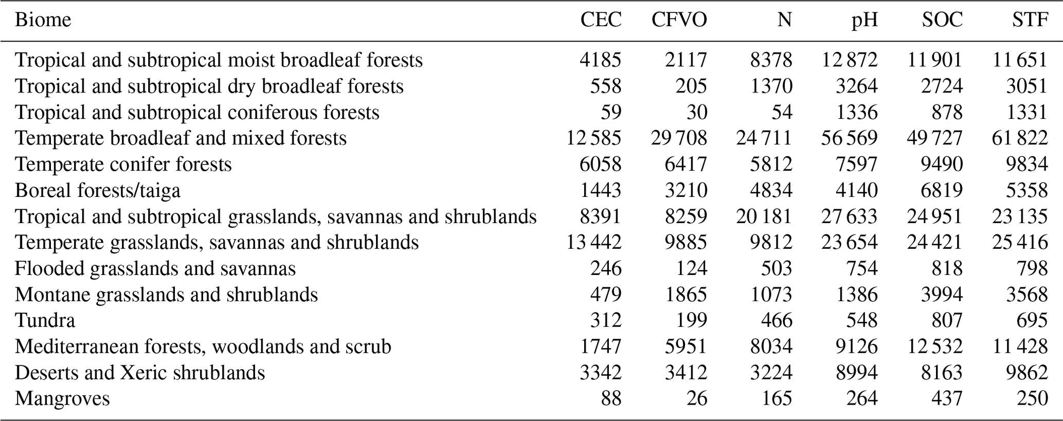
Table 2 breaks down the distribution of the legacy soil observations for each soil property by depth interval. Table B1, in Appendix B, shows the number of observations by bioclimatic region.

Figures 3 and 4 show examples of observation density of the soil calibration data for two soil properties, pH_water and proportion of coarse fragments, that show a large difference in density.

As indicated, the number of observations for each property varies greatly with depth and bioclimatic region, with higher densities observed for North America and Europe. Generally, there are more observations for agricultural areas. Further, the available profiles have been collated over several decades, some 62 % of the data being from 1960–2020; the time of sampling is unknown for around 34 % of the profiles. As indicated by  Batjes et al. (2020), in principle, the age of the observations should be taken into account during the mapping process via covariate layers for time periods commensurate with the sampling dates, especially for soil properties that are readily affected by changes in land use or management practices. However, for these so-called “dynamic” soil properties, such as pH and soil organic matter content, we consider that the spatial variation will be much greater that the temporal variation, so that not taking the age of observations into account will not greatly affect the map. In addition, it is difficult or impossible to find comparable covariates, in particular remote-sensing-derived covariates, for each time period. Space–time relations should be considered in future assessments (Heuvelink et al., 2020).

This study considers standardised data for some 240 000 profiles, derived from WoSIS. This is over 60 000 more profiles than considered in the data compilation underpinning the preceding SoilGrids runs (Hengl et al., 2017b), thus providing substantial new information for calibration of the new global models. However, as indicated, there are still significant geographic gaps (e.g. arid regions, boreal regions and “forest” soils). Some of these are related to the physical remoteness or inaccessibility of some regions, while others are related to the fact that many soil datasets still are not or can not be shared for various reasons as described by Arrouays et al. (2017).

Table 2 Number of observations per standard depth interval for each soil property. See Table 1 for abbreviations and units of the soil properties considered.

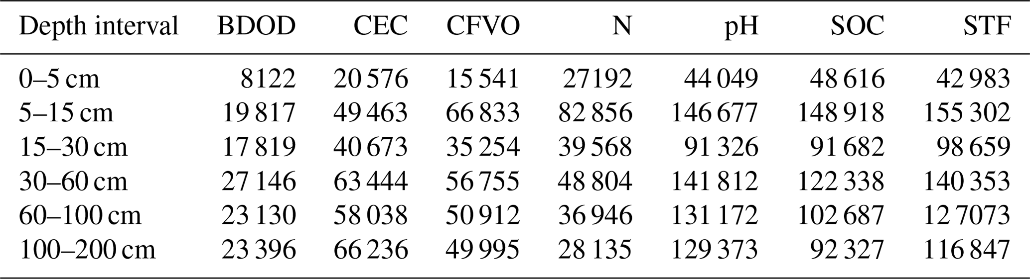
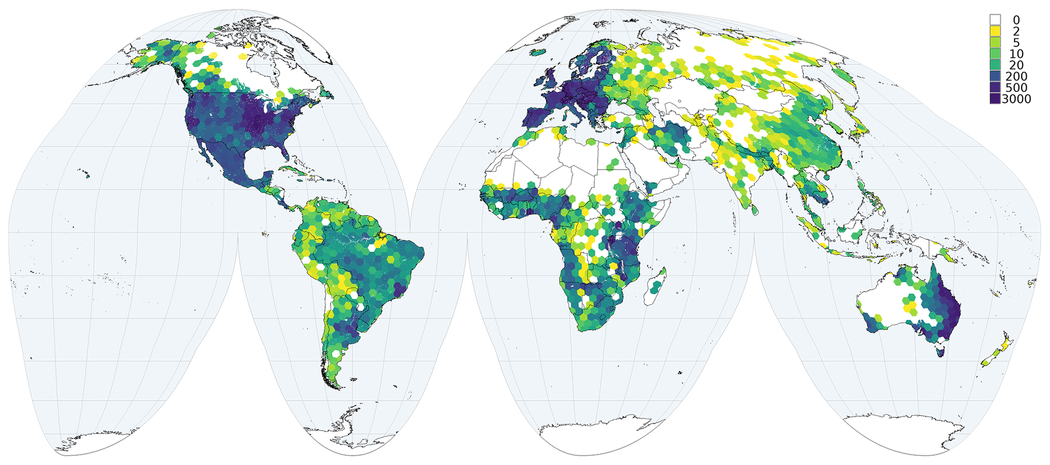
Figure 3 Number of observations per grid cell (70 000 km²) for soil pH_water.

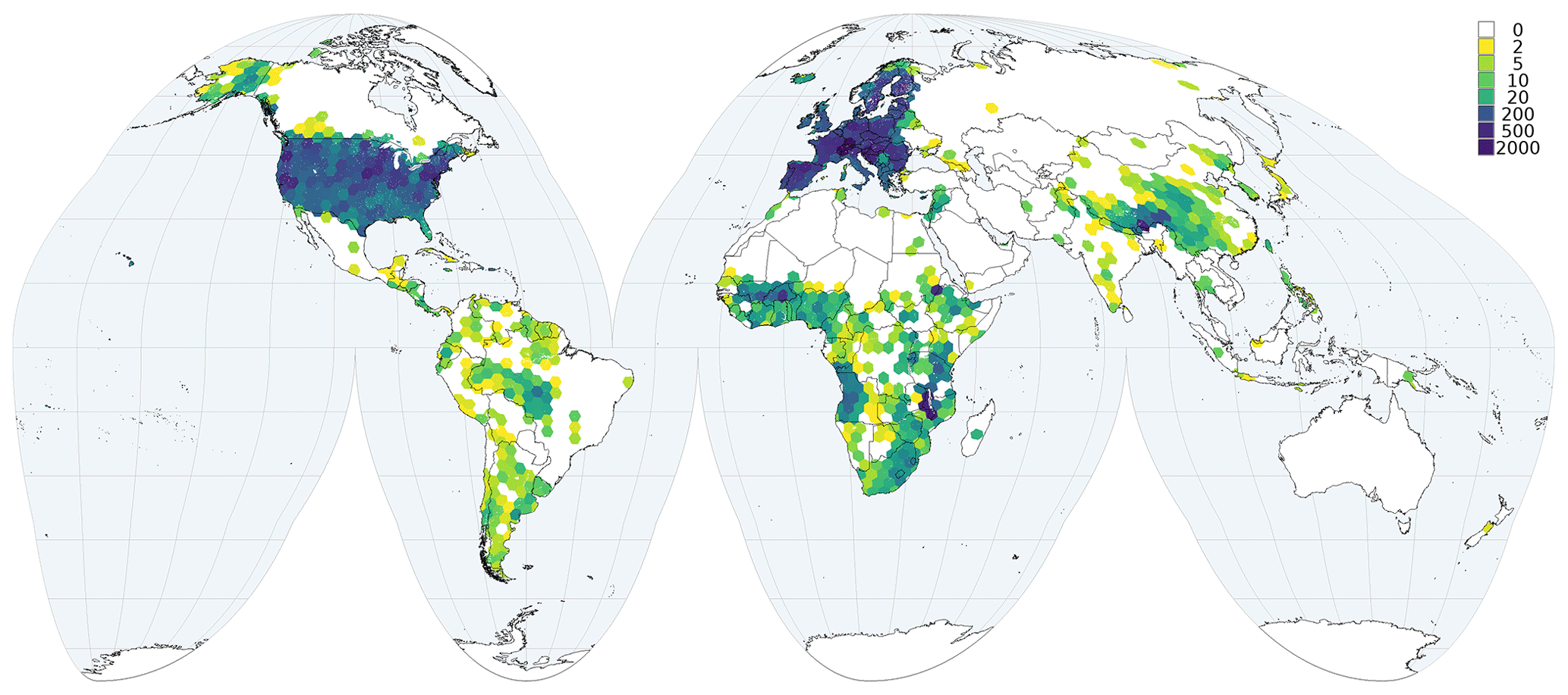
Figure 4 Number of observations per grid cell (70 000 km²) for coarse fragments.

In the previous version of SoilGrids (Hengl et al., 2017b), synthetic observations were randomly placed in regions with few or no observations, e.g. the Sahara and the Arabian Peninsula. This approach is worth further exploring, including information derived from other regional datasets, expert opinion and transfer learning from similar areas according to the Homosoil concept (Mallavan et al., 2010), which assumes similarity of soil-forming factors across regions. However, SoilGrids already implicitly incorporates the Homosoil concept, as long as there are sufficient observations in a given soil-forming environment anywhere in the world. Therefore, no synthetic observations (“pseudo-points”) were included in this version of SoilGrids, also by a lack of confidence about the accuracy of the synthetic data.

In future studies, it will be relevant to identify beforehand areas of the world with a low observation density that are not yet represented by a high density of observations in other areas with similar soil-forming factors. A set of synthetic profiles could then be generated to describe these areas, by consulting soil scientists knowledgeable on the soils and soil properties of these areas.

3.2 Model tuning and hyper-parameter selection

Model hyper-parameters selected for each property are presented in Table 3.

The numbers of covariates selected using the two-step approach for covariates' selection was fairly small in comparison with the full set (Table 3), resulting in more parsimonious models. Figure 5 shows two examples of the loss function for RFE for two soil properties with different numbers and distributions of input observations. In both cases, there is a clear improvement of performances while using 15 to 20 covariates. The curve reaches a minimum of the loss function and then stays on a plateau with a slight decline after the identified minimum.

All final models were trained with a maximum of 200 decision trees, a number beyond which performance gains did not noticeably increase.

The mtry parameter mainly depended on the number of covariates and was always between 1.5 and 2 times the square root of the number of covariates, which is the default provided by common random forest packages such as ranger (Wright and Ziegler, 2017). This confirms the need to determine optimum model hyper-parameters, especially when dealing with large numbers of input data (Nussbaum et al., 2018) as is the case here.

Table 3 Hyper-parameters for each considered soil property. See Table 1 for abbreviations and units of the soil properties considered.

Figure 5 Example of loss function (RMSE) used in the RFE step of covariates' selection.

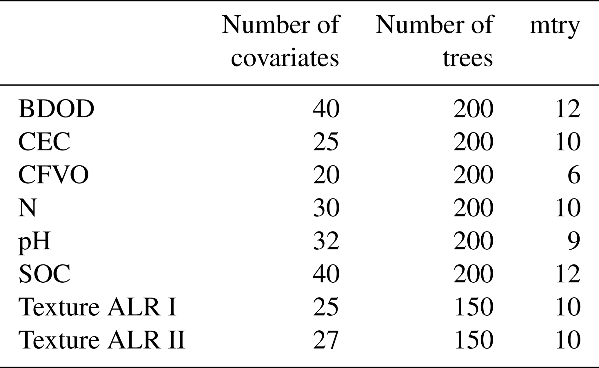
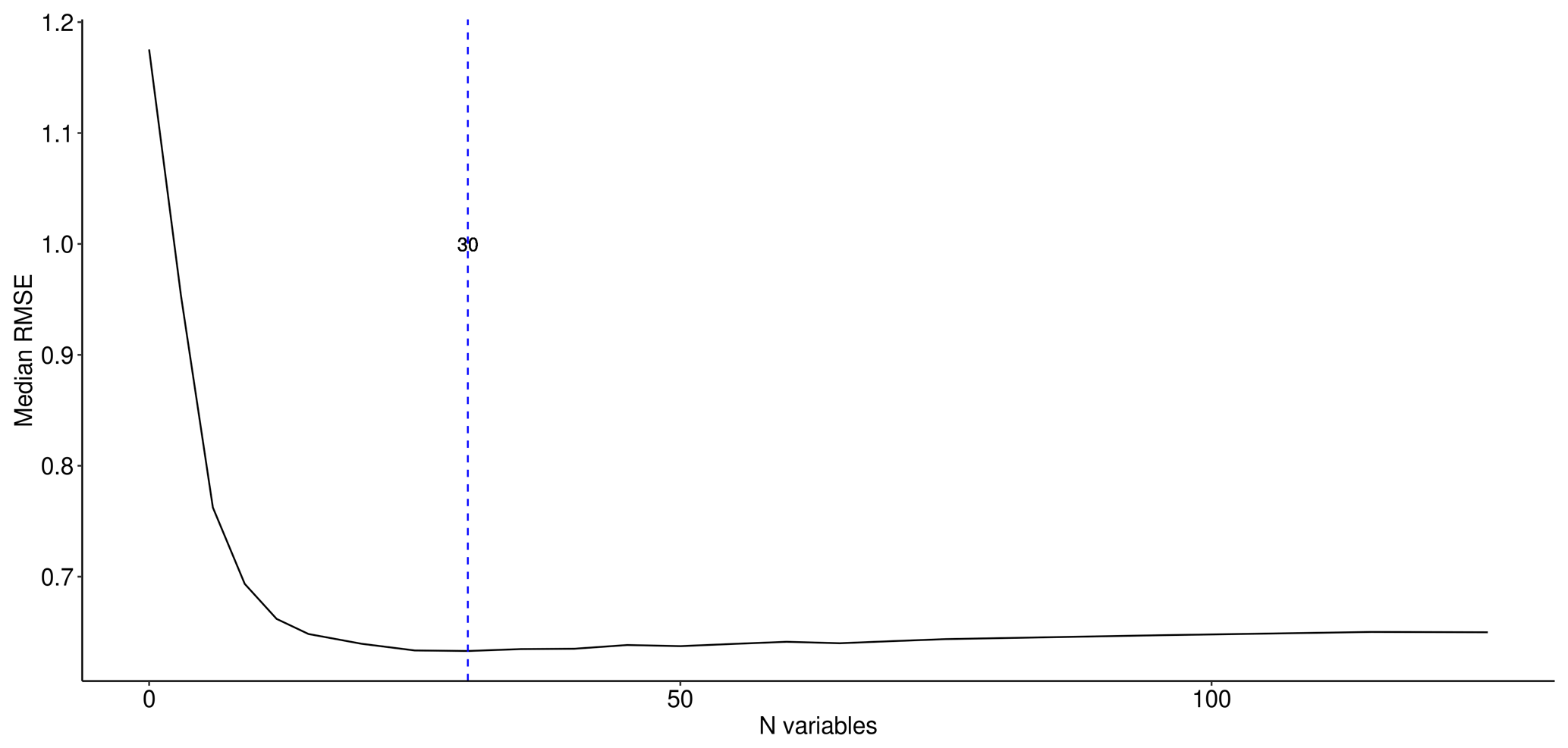
Table 4 Global cross-validation results for both mean and median predictions. See Table 1 for abbreviations and units of the soil properties considered.

Table 5 MEC per depth layer for mean predictions. See Table 1 for abbreviations and units of the soil properties considered.

Table 6 Prediction interval coverage probability, global and by predicted depth interval. See Table 1 for abbreviations and units of the soil properties considered.

3.3 Quantitative evaluation

Cross-validation results are summarised in Table 4, presenting the root mean squared error (RMSE) and model efficiency coefficient (MEC). The MEC varies from a minimum of 0.31 for coarse fragments to a maximum of 0.74 for BDOD. Clay is less well modelled than the other two particle-size classes. This may be an effect of the chosen ALR transformation that had clay as denominator (Lark and Bishop, 2007). Metrics of the mean were always better than or equal to those for the median for all properties.

Overall, these metrics are in line with continental or large-region DSM studies (Keskin and Grunwald, 2018). However, they are slightly lower than those presented by Hengl et al. (2017b). The latter difference can be explained by the more prudent cross-validation approach now taken, with spatially balanced folds and all observations belonging to the same profile in the same fold. This prevents the use of data from the same profile both for calibration and numerical evaluation.

Table 4 shows that the models with a higher number of retained covariates (Table 3) have better predictive performances. However, these models are also the models with the largest number of observations (Table 2). The considered soil properties are also different. Therefore, no general conclusion can be drawn from this observation.

Table 5 shows the MEC for mean predictions by depth interval. Performances decreased with depth, in line with many other DSM studies (Keskin and Grunwald, 2018). This pattern can be explained mainly by weakened relationships between environmental layers and soil properties of the deeper layers.

In this study, the vertical dimension of soil variability was only taken into account by using the depth of the observation as a covariate. Recent publications (Ma et al., 2021; Nauman and Duniway, 2019) indicate that such an approach can be too simplistic or lead to problems with consistency over the predicted depth sequence. This may be true for local datasets, in which the short-range spatial variability is of a similar magnitude as the vertical variability. Further research is necessary to assess the effects of using depth as a covariate on global datasets and models. Alternatives such as 3D smoothers (Poggio and Gimona, 2017b) or geostatistical models exploiting 3D spatial auto-correlation are worth exploring in further studies.

Table 6 summarises the PICPs, globally and by predicted depth interval. Most of the values are between 0.88 and 0.92, indicating that the prediction intervals obtained with QRF are a realistic representation of the prediction uncertainty, as the expected value for a 90 % prediction interval is 0.90. Exceptions are the models for coarse fragments with higher values around 0.95, indicating an overestimation of prediction uncertainty. The texture components have values with a larger spread, around 0.78 to 0.80 for sand and closer to 0.96 for silt and clay. These indicate a potential underestimation of prediction intervals for sand and overestimation for silt and clay. These results may be related with the range of these properties in the input observations. The transformation method used to derive the prediction intervals for the texture components could also be a contributing factor. Further exploration of the causes is worthwhile.

A key issue for DSM applications using legacy soil data is the evaluation of the results. The aspect of evaluation which compares actual with predicted values is numerical (or statistical) evaluation, often termed “validation” in the DSM literature; Oreskes (1998) and Rossiter (2017) explain why the term “evaluation” is preferred for the overall process of assessing the success of models, including DSM models. The best approach to numerical evaluation is to have an independent dataset obtained with probability sampling using a known sampling design (Brus et al., 2011; Brus, 2014). However, this is not feasible when only legacy data are available. In this case, a so-called “cross-validation” approach is often used. This needs to be tuned to avoid over- or underestimation of the numeric evaluation metrics, especially in case of large differences in observation density, i.e. clustered spatial observations. This is especially important at global scale, as the distribution of the soil observations is not uniform across the globe. It can not be guaranteed that the numeric evaluation metrics derived from cross-validation are unbiased estimates of the true numeric evaluation metrics, i.e. those that would have been computed on a probability sample of the whole population. It is also not possible to quantify how close the cross-validation metrics estimates are to the true metrics, as it is not possible to obtain confidence intervals (Brus et al., 2011). When using cross-validation it is important to prevent over- or under-optimistic estimates. For example, it is likely that prediction errors are smaller in areas where the sampling density is higher. Because of their high sampling density, such areas will be over-represented in the sample as the percentage of cross-validation points in clustered areas will be higher than the percentage of the total land area covered by those areas. Results of standard cross-validation will be strongly influenced by the performances in clustered areas. Using spatial cross-validation as suggested by Meyer et al. (e.g. 2018), where it is ensured that calibration data are never too close to a cross-validation point, on the other hand could produce over-pessimistic results. In order to address some of these concerns, this study adopted a practical solution in which the folds were created to guarantee a spatially balanced distribution between cross-validation folds, maintaining the same densities of the input data in each fold so that they represent approximately the same population.

Although the numerical evaluation procedure used in this work takes into account the spatial distribution of the observations and their density, further improvement is possible in both model training and evaluation. For example, the weights assigned to observations in heavily sampled areas could be reduced. The United States and large regions of Europe and Australia have high numbers of observations that could be downweighted to strengthen the spatial robustness of the evaluation procedure. Declustering or debiasing techniques (Goovaerts, 1997; Deutsch and Journel, 1998) have been applied with success in other geostatistics exercises and could be adapted to global soil mapping. The creation of the folds could also be modified to take into account the density of the observations.

3.4 Qualitative evaluation of spatial patterns

At global scale, well-known patterns are reproduced, and typical properties associated with many World Reference Base for Soil Resources (WRB) (IUSS Working Group WRB, 2015) Reference Soil Groups can be recognised.

For example, the pH map identifies the large regions of alkaline soils (Solonetz, Solochak), highly weathered soils (e.g. Acrisols, Alisols, Plithosols), acid forest soils (e.g. Podzols) and young soils from calcareous glacial deposits (e.g. Luvisols). The low pH of Andosols (e.g. Pacific Northwest United States, Japan, New Zealand) is also correctly represented. The texture components (particle size class – PSC) maps correctly identify the siltier deltas (e.g. Yellow–Yangtze, Ganges–Brahmaputra), broad river plains (e.g. Po, Danube, Mississippi, Rio Plate, upper Amazon), the loess regions (e.g. Midwestern United States, NW Europe, Ukraine) and the sandy North German–Polish plain. The cation exchange capacity (CEC) map clearly identifies large regions of highly weathered clays (e.g. Southeastern United States and China, central Brazil) and high-CEC 2:1 clays (e.g. “black cotton” Vertisols in the Deccan plateau and the Sudan). This map, together with the soil organic carbon (SOC) concentration maps, identifies large regions of Histosols (e.g. northern Canada, Scotland, Siberia, Borneo). The SOC stock map identifies deep Histosols and cool, wet regions (e.g. Pacific Northwest North American coast, Ireland, southern Chile). The coarse fragment map identifies large areas of the Tibetan Plateau and the principal mountain chains, as well as recently glaciated soils on igneous bedrock (e.g. Scandinavia, northern Quebec and Ontario).

Many regional patterns are also clear, for example the pH transition from Sahara through Sahel to the West African coast and the PSC transitions from the Des Moines glacial lobe to the proglacial loess deposits in Iowa (United States) as well as the PSC transition from clayey marine sediments along the North and Baltic Sea coasts through the sandy plains to the central German loess belt. The CEC map identifies contrasting areas of Vertisols (e.g, “black belts” in Alabama–Mississippi and Texas, United States). The coarse fragment map shows the detailed pattern of the basin-and-range region of the western United States and the ridge-and-valley region of Appalachia.

However, at the local scale, a preliminary assessment of SoilGrids in the United States, compared with a gridded version of the national detailed gSSURGO (NRCS National Soil Survey Center, 2016) soil geographic database based on a detailed field survey, reveals that SoilGrids may fail to account for local parent material transitions, e.g. sedimentary facies of coastal plain marine sediments, as well as glacial features such as proglacial lacustrine sediments and relic beach lines, so that the local PSC pattern is not accurate, sometimes on the order of 20 %–30 % of a particle-size class.

For example, Fig. 6a shows predicted sand concentration of the 0–5 cm layer in an approximately 50×50 km area in central Pennsylvania (United States), ranging from approximately 25 % (darkest red) to 80 % (darkest blue). Important local differences are clear: the low sand concentrations of the clayey soils in the limestone valleys trending SW–NE and the high concentrations in soils from glacial till developed on sandstones in the north, as well as the residual soils on the resistant sandstone ridges of the Ridge and Valley province of Appalachia in the south. These do generally agree with the detailed soil survey.

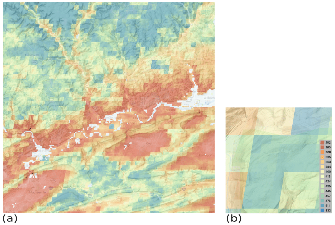
Figure 6 Predicted sand concentration, %, 0–5 cm, ground overlay in © Google Earth. (a) Overview; centre $\approx -$77^∘14^′ E, 41^∘14^′ N, near Jersey Shore, PA. (b) Detail; centre $\approx -$76^∘56^′ E, 41^∘33^′ N.

At the detailed scale (250 m pixel), SoilGrids typically shows fine details that do not always appear to be related to obvious landscape or land use differences, when the map is viewed as a ground overlay in Google Earth. For example, Fig. 6b shows detail of predicted sand concentration of the 0–5 cm layer in an approximately 3×3 km area of the previous figure. The effect of some covariates being at 1 km resolution and others at 250 m is apparent, but the reason for the fine-scale differences is not. This area is of similar lithology, relief and land cover (second-growth dense forest) except the narrow valley at the north-west edge, yet the predictions are quite different.

In this context, it should be realised that SoilGrids250m predictions are not meant for use at a detailed scale, i.e. at the subnational or local level, as national data providers often have access to more detailed point datasets and covariate layers for their country than have been provided to the point dataset on which SoilGrids250m is based (Chen et al., 2020; Roudier et al., 2020; Vitharana et al., 2019; Liu et al., 2020).

3.5 Prediction uncertainty

In general, the least sampled areas present the highest prediction uncertainties as expressed by the PICP. Figures 7 and 8 show an example for two properties and depths (maps for all properties and depths can be accessed at https://data.isric.org). Figure 9 and 10 show an example representing the quantiles for pH_water for the 60–100 cm layer. The north of Russia and the centre and north-west of Canada are large regions for which few soil observations are available; therefore prediction distributions are wider than in more densely sampled areas. However, these patterns are different for different properties. For example, arid areas actually have the narrowest prediction ranges of pH_water. The uncertainty range is often wide for properties and regions with a wider range of the property being modelled. This can be explained by the modelling approach performing more accurately within a limited range of options. These regions also have larger local spatial variation with more difficulties for predictions.

The communication of uncertainty is an open challenge (Arrouays et al., 2020). Uncertainty should provide information for policymakers and other stakeholders and not only scientists and modellers. The maps computed with Eq. (3) are a first step in this direction, but their limitations must be understood. For properties that have values at or near zero, e.g. coarse fragments, they do not provide an entirely accurate uncertainty estimate. The use of uncertainty classes could be a further step to help domain stakeholders.

Figure 7 Mean soil organic carbon content (dg/kg) prediction and range between 5 % and 95 % quantiles in the 5 to 15 cm depth interval, (a) for prediction and (b) for interquartile range.

Figure 8 Median total nitrogen prediction (cg/kg) and associated uncertainty for the 15 to 30 cm depth interval, (a) for prediction and (b) for uncertainty.

3.6 Limitations and outlook

This study represents a considerable effort to provide a globally consistent product using the point dataset available to ISRIC, a large number of relevant covariates and some optimisation of a well-established machine learning method, within the limits of practical computation. Yet it is clear that this product has some limitations, which will be considered in further work.

First, there is an ever-expanding group of new covariates that can help explain and model the spatial variation of soil properties. Products derived from Earth observation are particularly relevant in this regard and have considerably improved over the last decade. For example, the European Space Agency Sentinel missions (both optical and radar) provide high-resolution data that have been shown to improve DSM model performances.

Second, a fundamental problem is a lack of well distributed point observations within the soil property geographic and features space. Additional soil data for so far under-represented regions, for example the northern boreal regions as being collated by the International Soil Carbon Network (Malhotra et al., 2019), will be sought for possible consideration in the WoSIS workflow that provides the point data underpinning the SoilGrids mapping effort. This effort would be aided by the provision by more data providers of at least a representative part of their point data to WoSIS, under suitable license. It is also important to consider the distribution of the observations in the covariate space to minimise the issues related to predictions into unknown regions of feature space (Meyer and Pebesma, 2020).

Figure 9 Prediction distribution for pH_water (10 pH) in the 60 to 100 cm depth interval, (a) for mean and (b) for median.

Figure 10 Prediction distribution for pH_water (10 pH) in the 60 to 100 cm depth interval, (a) for 5 % quantile and (b) for 95 % quantile.

Third, DSM methods are under active development, both new methods and improvements to established methods. The use of decision-tree-based models in DSM has become fairly common in recent years. Models such as random forests, XGBoost or Cubist tend to provide better results than most multiple linear regression methods with reasonable computation costs (Khaledian and Miller, 2020). However, methods such as artificial neural networks promise further improvements in model performances if the amount and distribution of the data support these highly complex models. This is the case in particular with convolutional or recursive neural networks (deep learning). However, these methods present computational challenges with the amount of training data necessary for a sufficiently accurate DSM exercise, especially when working at global scale at medium to fine resolutions.

Fourth, the proper method of cross-validation is another important aspect when considering how to assess and improve model performances. In particular, spatial cross-validation and declustering of the data need to be further explored.

Fifth, this research considered only the modelling of some primary soil properties, as defined and described in the GlobalSoilMap specifications. More work is necessary to obtain maps for soil thickness (either rooting zone, pedogenetic solum or regolith), soil properties derived with pedo-transfer functions, e.g. hydrologic soil properties such as saturated hydraulic conductivity (Pachepsky and Rawls, 2004), and complex properties that depend on multiple primary properties, e.g. carbon stocks. These layers are important inputs to model and map soil functions in the present and in the future as well as to support Earth system modelling (Luo et al., 2016; Dai et al., 2019).

Sixth, the quantification of uncertainty is recommended and is becoming more common in DSM studies. This work introduced it at global scale for the first time to the best of our knowledge. While the provision of quantiles is mentioned in the GlobalSoilMap specifications, the representation and communication of uncertainty to end users and stakeholders remain an important research field to be further explored. The appropriate uncertainty intervals, both in terms of user acceptance and modelling feasibility, also need to be investigated.

Finally, the integration of highly automatised workflows with expert opinion should be further explored. DSM products use statistical models to describe soils, and it is important to take into account the expertise and experience of pedologists, at least in an evaluation loop if not as part of the modelling itself. We made a first attempt at this in the Qualitative evaluation section above but do not have a method to effectively incorporate expert observations into a workflow.

4 Conclusions

This study presents and discusses the production of global maps of soil properties as implemented in the SoilGrids 2.0 product, with cross-validation, hyper-parameter selection and quantification of uncertainty, using the best available (shared) soil profile data for the world. In particular, the study describes a robust and reproducible DSM workflow addressing the challenges of global data modelling:

1. non-homogeneous spatial distribution of input soil observations;

2. robust quantitative evaluation with a cross-validation procedure balancing accuracy and performances;

3. qualitative evaluation of the spatial patterns of the maps to include information about matching with well recognised pedo-landscape features;

4. quantification and mapping of the spatial uncertainty to provide users with a measure for and warning for users of the products.

As such, it describes a next step into global modelling and mapping of soil properties, explicitly highlighting the importance of quantitative and qualitative evaluation and uncertainty communication. The actual use of SoilGrids 2.0 in global and wide-area regional applications, where soil properties are important model inputs, will be the real test of its applicability and usefulness.

Appendix A: Environmental covariates

Over 400 geographic layers were available as environmental covariates for this work. These are chosen for their presumed relation to the major soil forming factors.

(Karger et al., 2016)(Bontemps et al., 2013)(Wilson and Jetz, 2016)(Wan, 2006)(Fick and Hijmans, 2017)(Dinerstein et al., 2017)(Pelletier et al., 2016)(Hartmann and Moosdorf, 2012)(Bontemps et al., 2013)(Hansen et al., 2013)(Chen et al., 2015)(Robinson et al., 2014)(Reuter and Hengl, 2012)(Sayre et al., 2014)(Zanter, 2019)(Savtchenko et al., 2004)(Zanter, 2019)(Savtchenko et al., 2004)(Fluet-Chouinard et al., 2015)(Pekel et al., 2016)(Fan et al., 2013)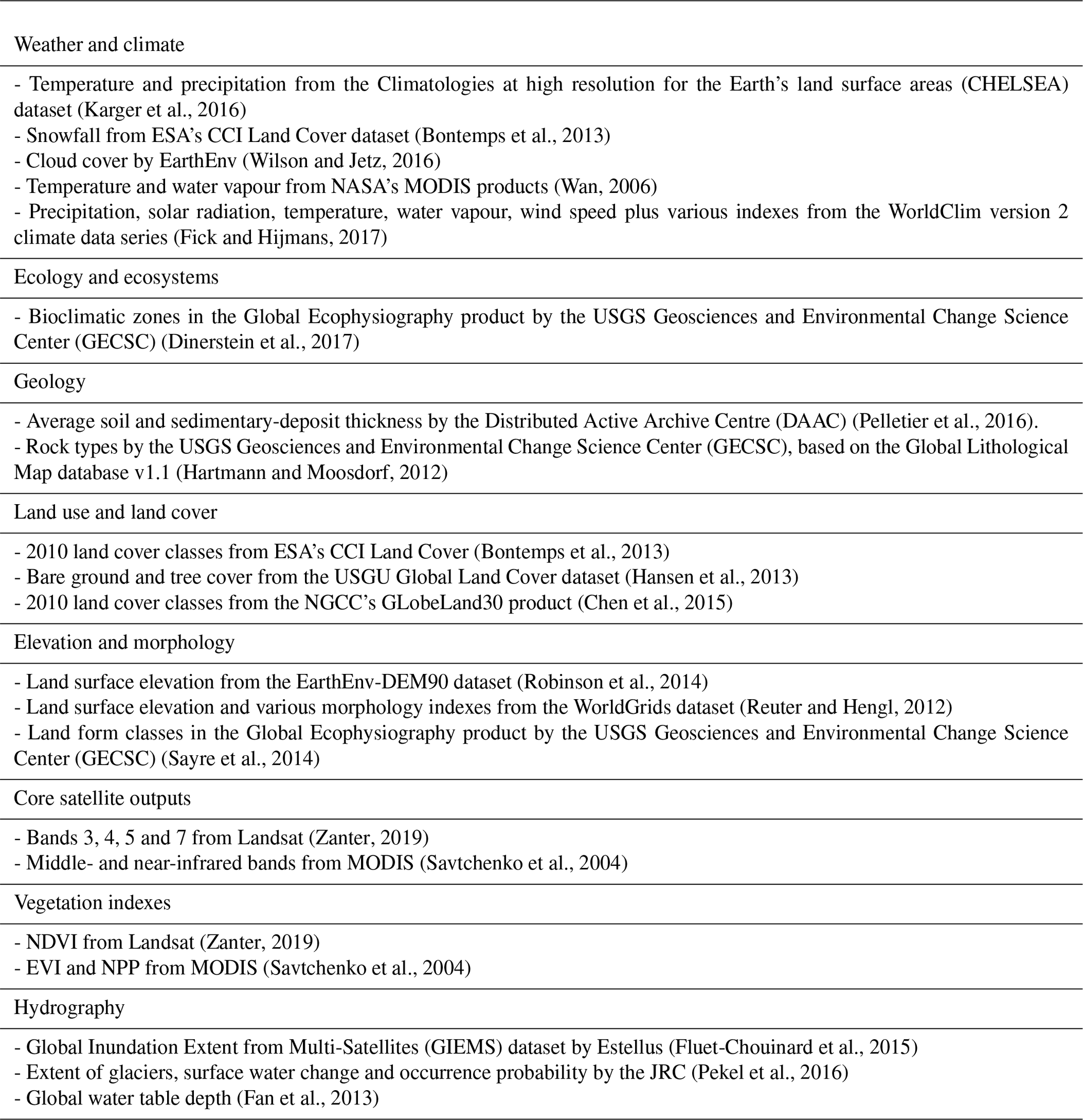

Table A1 Covariate sets and sources.

Appendix B: Bioclimatic regions

Table B1 summarises the number of observations per property for each bioclimatic region. An interactive map of the regions is available at http://ecoregions2017.appspot.com/ (last access: 20 May 2021).

Table B1 Number of observations per property for each bioclimatic region. See Table 1 for abbreviations.