the Creative Commons Attribution 4.0 License.
the Creative Commons Attribution 4.0 License.
 | 06 Mar 2020
Time-lapse monitoring of root water uptake using electrical resistivity tomography and mise-à-la-masse: a vineyard infiltration experiment
Luca Peruzzo
Jacopo Boaga
Nicola Cenni
Myriam Schmutz
Susan S. Hubbard
Giorgio Cassiani
This paper presents a time-lapse application of electrical methods (electrical resistivity tomography, ERT; and mise-à-la-masse, MALM) for monitoring plant roots and their activity (root water uptake) during a controlled infiltration experiment. The use of non-invasive geophysical monitoring is of increasing interest as these techniques provide time-lapse imaging of processes that otherwise can only be measured at few specific spatial locations. The experiment here described was conducted in a vineyard in Bordeaux (France) and was focused on the behaviour of two neighbouring grapevines. The joint application of ERT and MALM has several advantages. While ERT in time-lapse mode is sensitive to changes in soil electrical resistivity and thus to the factors controlling it (mainly soil water content, in this context), MALM uses DC current injected into a tree stem to image where the plant root system is in effective electrical contact with the soil at locations that are likely to be the same where root water uptake (RWU) takes place. Thus, ERT and MALM provide complementary information about the root structure and activity. The experiment shows that the region of likely electrical current sources produced by MALM does not change significantly during the infiltration time in spite of the strong changes of electrical resistivity caused by changes in soil water content. Ultimately, the interpretation of the current source distribution strengthened the hypothesis of using current as a proxy for root detection. This fact, together with the evidence that current injection in the soil and in the stem produces totally different voltage patterns, corroborates the idea that this application of MALM highlights the active root density in the soil. When considering the electrical resistivity changes (as measured by ERT) inside the stationary volume of active roots delineated by MALM, the overall tendency is towards a resistivity increase during irrigation time, which can be linked to a decrease in soil water content caused by root water uptake. On the contrary, when considering the soil volume outside the MALM-derived root water uptake region, the electrical resistivity tends to decrease as an effect of soil water content increase caused by the infiltration. The use of a simplified infiltration model confirms at least qualitatively this behaviour. The monitoring results are particularly promising, and the method can be applied to a variety of scales including the laboratory scale where direct evidence of root structure and root water uptake can help corroborate the approach. Once fully validated, the joint use of MALM and ERT can be used as a valuable tool to study the activity of roots under a wide variety of field conditions.
- Article
(11028 KB) - Full-text XML
- Companion paper
- BibTeX
- EndNote


The interaction between soil and biota is one of the main mechanisms controlling the exchange of mass and energy between the Earth's terrestrial ecosystems and the atmosphere. Philip (1966) was the first to use the phrase “soil–plant–atmosphere continuum” (SPAC) to conceptualize this interface in the framework of continuum physics. Even though more than five decades have elapsed and many efforts have been expanded (e.g. Maxwell et al., 2007; de Arellano et al., 2012; Anderegg et al., 2013; Band et al., 2014), the current mechanistic understanding or modelling of SPAC is still unsatisfactory (e.g. Dirmeyer et al., 2006, 2014; Newman et al., 2006). This is not totally surprising, since soil–plant interactions are complex, exhibiting scale and species dependence with high soil heterogeneity and plant growth plasticity. In this study, we focus on new methods designed to image root systems and their macroscopic functioning, in order to help understand the complex mechanisms of these systems (the rhizosphere, e.g. York et al., 2016). This diversity of interactions presents an enormous scientific challenge to understanding the linkages and chain of impacts (Richter and Mobley, 2009).
Roots contribute substantially to carbon sequestration. Roots are the connection between the soil, where water and nutrients reside, to the other organs and tissues of the plant, where these resources are used. Hence roots provide a link in the pathway for fluxes of soil water and other substances through the plant canopy to the atmosphere (e.g. Dawson and Stiegwolf, 2007). These transpiration fluxes are responsible for the largest fraction of water leaving the soil in vegetated systems (Chahine, 1992). Root water uptake (RWU) influences the water dynamics in the rhizosphere (Couvreur et al., 2012) and the partitioning of net radiation into latent and sensible heat fluxes, thereby impacting atmospheric boundary layer dynamics (Maxwell et al., 2007; de Arellano et al., 2012). Yet, a number of issues remain when representing RWU in both hydrological and atmospheric models. Dupuy et al. (2010) summarize the development of root growth models from its origins in the 1970s with simple spatial models (Hackett and Rose, 1972; Gerwitz and Page, 1974) to the development of very complex plant architectural models (Jourdan and Rey, 1997). Dupuy et al. (2010) advocate for a different approach, where root systems are described as density distributions. Attempts in this direction (Dupuy et al., 2005; Draye et al., 2010; Dupuy and Vignes, 2012) require much less specific knowledge of the detailed mechanisms of meristem evolution and yet are sufficient to describe the root functions in the framework of continuum physics, i.e. the one endorsed by the SPAC concept. These models also lend themselves more naturally to calibration against field evidence, as they focus on the functioning of roots, especially in terms of RWU (e.g. Volpe et al., 2013; Manoli et al., 2014). However, calibration requires that suitable data such as root density and soil water content evolution are available in a form comparable with the model to be calibrated. This is the main motivation behind the work presented herein.
A thorough understanding of root configuration in space and their evolution in time is impossible to achieve using only traditional invasive methods: this is particularly true for root hairs, i.e. for the absorptive unicellular extensions of epidermal cells of a root. These tiny, hair-like structures function as the major site of water and mineral uptake. Root hairs are extremely delicate, turn over quickly, and are subject to desiccation and easily destroyed. For these reasons, direct investigation of their in situ structure via excavation is practically impossible under field conditions.
The development of non-invasive or minimally invasive techniques is required to overcome the limitations of conventional invasive characterization approaches. Non-invasive methods are based on physical measurements at the boundary of the domain of interest, i.e. at the ground surface and, when possible, in shallow boreholes. Non-invasive methods provide spatially extensive, high-resolution information that can also be supported by more traditional local and more invasive data such as soil samples, time-domain reflectometry (TDR), lysimeters and rhizotron measurements.
Electrical signals may contribute to the detection of roots and to the characterization of their activities. For instance, self-potential (SP) signals can be associated with plant activities: water uptake generates a water circulation and a mineral segregation at the soil–root interface that induces ionic concentration gradients which in turn generate voltages of the order of a few millivolts (Gibert et al., 2006). However, such SP sources are generally too low to be detectable in the normally noisy environment.
Induced polarization (e.g. Kemna et al., 2012) is also a promising approach in root monitoring. This is consistent with the fact that root systems are commonly modelled as electrical circuits composed of resistance R and capacitance C (e.g. Dalton, 1995 and similar models). Recently, Mary et al. (2017) considered polarization from soil to root tissues, as well as the polarization processes along and around roots, to explain the phase shift (between injected current and voltage response) observed for different soil water content. Weigand and Kemna (2017, 2019) demonstrated that multi-frequency electrical impedance tomography is capable of imaging root system extent.
In the investigation of roots and RWU the most widely used non-invasive technique is electrical resistivity tomography (ERT – e.g. Binley and Kemna, 2005). ERT measures soil electrical resistivity and, in time-lapse mode, resistivity changes over time. Electrical resistivity values depend on soil type and its porosity but also on state variables such as the saturation of electrolytes (water) in the pores and the concentration of solutes in the pore water (as described for example by the classical Archie law, 1942). Note, however, that other factors may play a role, such as clay content (Rhoades et al., 1976; Waxman and Smits, 1968) and temperature (e.g. Campbell et al., 1949). However, in general, it is possible to estimate water content changes from changes in electrical resistivity over time (and space), provided that pore water salinity does not vary dramatically. While ERT has been attempted for quantifying root biomass on herbaceous plants (e.g. Amato et al., 2009), the main use of this technique in this context aims at identifying changes in soil water content in space and evolution in time (e.g. Michot et al., 2003, 2016; Srayeddin and Doussan, 2009; Garré et al., 2011; Cassiani et al., 2012; Brillante et al., 2015). With specific reference to RWU, Cassiani et al. (2015, 2016), Consoli et al. (2017) and Vanella et al. (2018) used time-lapse ERT with 3D cross-hole configurations to monitor changes in soil electrical resistivity caused by irrigation and RWU for different crops (apple and citrus trees). It should also be noted that RWU and the release of different exudates by fine roots modify soil water content and resistivity at several temporal scales (York et al., 2016).
On the other hand, evidence suggests that roots themselves may produce signals in ERT surveys (Amato et al., 2008; Werban et al., 2008); however, these signals are often difficult to separate from soil heterogeneities and soil water content variations in space (Rao et al., 2019). Nevertheless, in most cases, the ranges of electrical resistivity of soil and roots overlap, and while the amplitude of contrasts varies according to the soil resistivity and tree species (e.g. Mary et al., 2016), the direct identification of root systems using ERT is often impractical.
Recently, the mise-à-la-masse (MALM) method has been proposed for plant root mapping. MALM is a classical electrical method (Parasnis, 1967) originally developed for mining exploration but also used more recently for example in the context of landfill characterization (De Carlo et al., 2013) as well as conductive tracer test monitoring (Osiensky, 1997; Perri et al., 2018). In MALM, an electrical current is injected into a conductive body with a return current electrode far away (at infinity), and the resulting voltage is measured at the ground surface or in boreholes, again with a reference electrode at infinity: the shape of voltage contour lines is informative about the extent and orientation of the conductive body. This idea can be applied to the plant stem and root system, considering that electrical current can be transmitted through the xylem and phloem (on either side of the cambium), where sap flow takes place. The main assumption is that fine root connections and mycorrhiza at the contact between roots and soil convey the injected current into the soil where this contact is efficient, thus appearing as a distribution of current sources in the ground. The location of these sources should correspond to the locations of active contacts between roots and soil and could be identified starting from the measured voltage distribution at the ground surface or in boreholes. This approach has been recently tested by Mary et al. (2018, 2019) on vine trees and citrus trees, showing that current injection in the stem and in the soil just next to the stem produces very different voltage patterns, thus confirming that the stem–root system conveys current differently from a direct injection in the ground.
In this study we present the results of an infiltration experiment conducted in a Bordeaux vineyard (France). This paper is meant to be an extension of Mary et al. (2018) and to focus on the results of an infiltration experiment. The experiment was monitored (also) using time-lapse 3D ERT and time-lapse MALM measurements, the latter performed by injecting current into the vine trees stems. This study had the following goals:
- a.
define a non-invasive investigation protocol capable of imaging the root activity as well as the distribution of active roots, at least in terms of their continuum description mentioned above, under varying soil water content conditions;
- b.
integrate the geophysical results with mass flux measurements in/out of the soil–plant continuum system using a simple 1D simulation reproducing the infiltration experiment; and
- c.
give recommendations for future experiments focusing on the method validation.
2.1 Site description
The study was conducted in a commercial vineyard (Château La Louvière, Bordeaux) in the Pessac-Léognan appellation of France (44∘44′15′′ N, 0∘34′45′′ W). The climate of the region is oceanic with a mean annual air temperature of 13.7 ∘C and about 800 mm annual precipitation. Grapevine trees are planted at 1 m distance along the rows, and the rows are spaced about 1.5 m. We focused our interest on two neighbouring plants.
The vineyard is not irrigated. The soil is sandy down to 1 m depth with sandy clay below, down to 1.75 m, and calcareous at depth. Due to its larger particles and thus smaller surface area, the sandy layer has a relatively poor water retention capacity. Nevertheless, the water supply of the vine plant is not a limiting factor (refer to Fig. 2 and Mary et al., 2018, for more details about the plants and soil type). We concentrated our monitoring on only two neighbouring grapevines (Fig. 1), which differ in age and size: plant A was smaller and younger, and plant B was considerably larger and older.

Figure 1Picture of the field site in May 2017 (a), wired plants investigated (b), and grape status during the experiment in June 2017 (c).
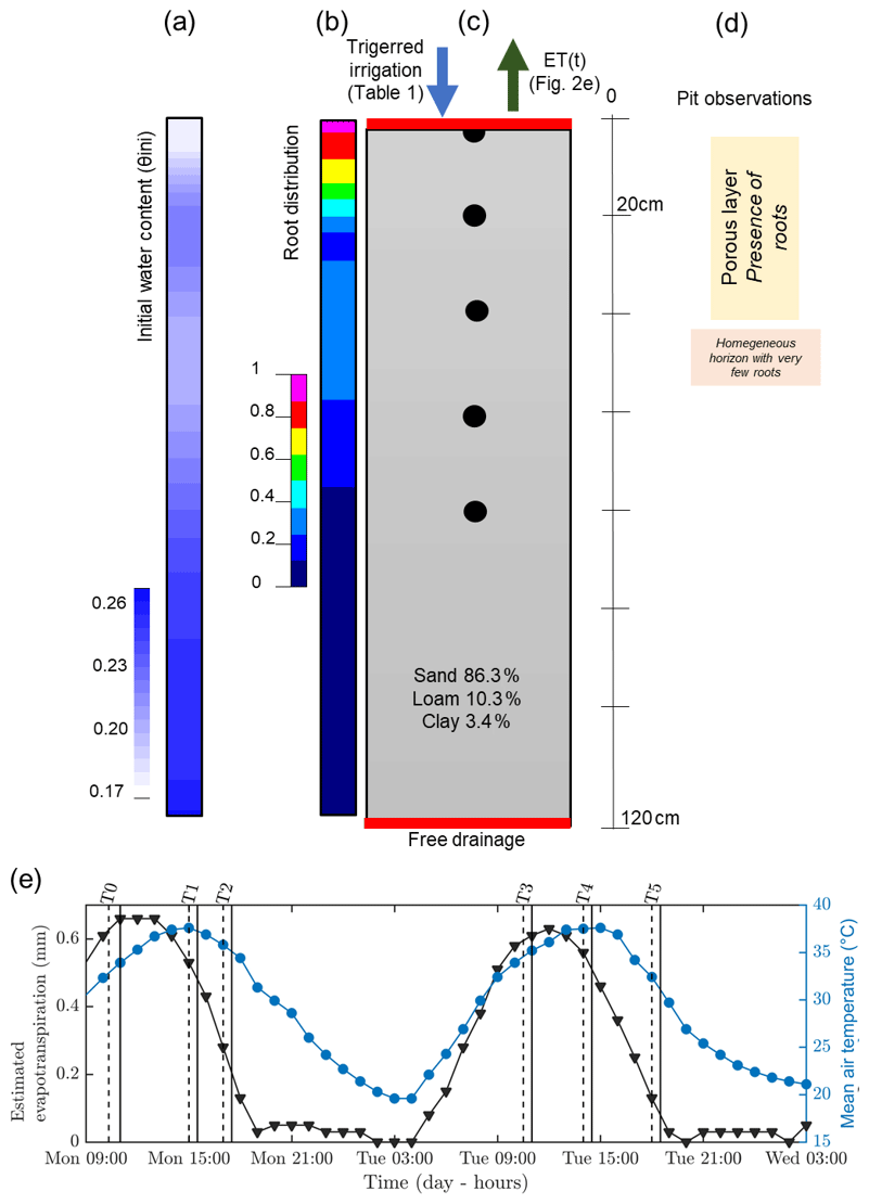
Figure 2Initial (a, b, c) and time-varying atmospheric conditions used for the hydrological simulation. From left to right: (a) initial conditions on soil water content θini, (b) root density (1 cm−1), (c) soil type, and (d) pit observations. (e) Variation of temperature (blue line) and estimated evapotranspiration (black line) derived from a nearby meteorological station. The vertical lines indicate acquisition times for plant A (dashed and plain line respectively for the start and the end of the measurement; see Table 1).
2.2 Meteorological measurements and irrigation schedule
Hourly meteorological data were acquired by an automatic weather station located about 300 m from the plot and managed by DEMETER (agrometeorological service – http://www.meteo-agriculture.eu/qui-sommes-nous/lhistoire-de-demeter, last access: 22 January 2020). These micrometeorological data were valuable to estimate the initial soil conditions and the changes in time (Fig. 2). Potential evapotranspiration (ETP) was computed according to the Penman–Monteith formula accounting for the incoming short-wave solar radiation, air temperature, air humidity, wind speed and rainfall measured by the station. Prior to 19 June 2017, date of the first field data acquisition, little precipitation was recorded for 5 d (only 2.5 mm on 13 June) and only 18 mm cumulative precipitation was recorded during the entire month of June 2017. The mean air temperature was very high (35 ∘C under a well-ventilated shelter). Consequently, the plants were probably suffering from water deficit at the time of the experiment. Thus, at the start of the experiment, we assumed that the soil water content (SWC) around the plants was probably below to field capacity. As shown in Fig. 2, the evapotranspiration rate was about 5.6 mm d−1.
The controlled infiltration experiment was conducted using a sprinkler installed between the two monitored plants, placed at an elevation of 1.4 m, in order to apply irrigation water as uniformly as possible. The irrigation started on 19 June 2017 at 13:00 LT and ended 2 h later (15:00 LT) for a total of 260 L (104 L h−1). Runoff was observed due to topography and probably induced more water supply for plant A, which is located downhill. The irrigation water had an electrical conductivity of 720 µS cm−1 at 15 ∘C.
2.3 ERT and MALM data acquisition
We carried out a time-lapse ERT acquisition, based on custom-made ERT boreholes (six of them, each with 12 electrodes), plus surface electrodes (Fig. A1 in Appendix A). The six boreholes were placed to form two equal rectangles at the ground surface. Each rectangle size was 1 m by 1.2 m respectively in the row and inter-row line directions, with a vine tree placed at the centre of each rectangle. The boreholes were installed in June 2015, and a good electrical contact with soil had already been achieved at the time of installation. The topmost electrode in each hole was 0.1 m below ground, with vertical electrode spacing along each borehole equal to 0.1 m. In each rectangle, 24 surface stainless steel electrodes (14 mm diameter), spaced 20 cm in both horizontal directions, surrounded the plant stem arranged in a five by five regular mesh (with one skipped electrode near the stem). Note that after testing smaller electrode sizes in the surface, we finally adopted larger ones since they ensured a better contact in the loose soil and were heavier and more firmly grounded (3 cm out of 12) to resist irrigation. We conducted the acquisitions on each rectangle independently. Each acquisition was therefore performed using 72 electrodes (24 surfaces and 48 electrodes in four boreholes) and an IRIS Syscal Pro resistivity meter. For all measurements we used a skip 2 dipole–dipole acquisition (i.e., a configuration where the current dipoles and potential dipoles are 3 times larger than the minimal electrode spacing). The total dataset includes three types of measurements: 430 surface-to-surface, 2654 surface-to-borehole and 4026 in-hole measurements.
In addition to acquiring ERT data, we also acquired MALM data. MALM acquisition was logistically the same as ERT and was supported by the same device but used a pole-pole scheme (with two remote electrodes). Borehole and surface electrodes composing the measurement set-up were used as potential electrodes, while current electrode C1 was planted directly into the stem, 10 cm from the soil surface, with an insertion depth of about 2 cm, in order to inject current directly into the cambium layer. The two remote electrodes C2 (for current) and P2 (for voltage) were placed approximatively at a 30 m distance from the plot, in opposite directions. Note that for MALM (unlike for ERT) one corner surface electrode was put near the stem in order to refine the information at the centre of each rectangle.
Each MALM acquisition was accompanied by a companion MALM acquisition where the current electrode C1 was placed directly in the soil next to the stem rather than in the stem itself. In this way the effect of the plant stem–root system in conveying current can be evidenced directly comparing the resulting voltage patterns resulting from the two MALM configurations.
For both ERT and MALM, we acquired both direct and reciprocal configurations (that swap current and voltage electrode pairs) in order to assess the reciprocal error as an estimate of measurement error (see e.g. Cassiani et al., 2006). Note that, for the MALM case, reciprocals may not be the best solutions to estimate data quality as it has been shown in Mary et al. (2018), possibly because of non-linearity caused by current injection in the stem.
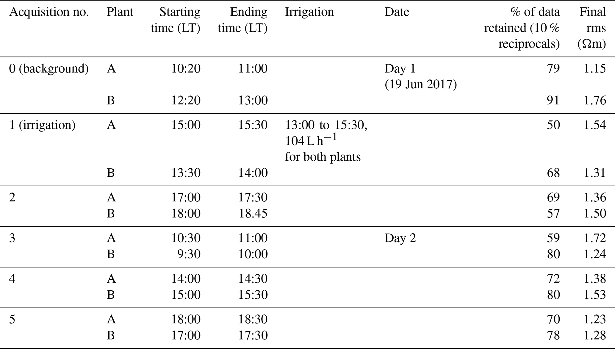
We adopted a time-lapse approach, conducting repeated ERT and MALM acquisitions over time in order to assess the evolution of the system's dynamics under changing moisture conditions associated with the infiltration experiment. We conducted repeated measurements starting on 19 June 2017 at 10:20 LT and ending the next day at about 17:00 LT. The schedule of the acquisitions and the irrigation times is reported in Table 1.
Table 1Schedule of the acquisitions and the irrigation times; plant A and B are measured consecutively and consist each time of three measurements: ERT, MALM stem and MALM soil. Assessment of data and inversion quality from the two last columns, i.e. respectively the percentage of data that passed the reciprocity (analysis at 10 %) and rms error at the end of the inversion.
2.4 Forward hydrological model and comparison with geophysical results
Hydrus-1D (Simunek et al., 1998) was used to simulate cumulative infiltration and water content distributions for plant B (the larger one). The results from geophysical data acquisition were used to feed the hydrological model initial conditions. Boundary conditions were set for the column respectively as an atmospheric BC with surface runoff (observed during the experiment) and triggered irrigation for the upper part and free drainage for the lower part (see Fig. 2). We assumed that the retention and hydraulic conductivity functions can be represented by the Mualem–van Genuchten model (MVG, Mualem, 1976; van Genuchten, 1980). Soil hydraulic parameters were directly inferred using grain size distribution and the pedotransfer functions from the Rosetta software (Schaap et al., 2001). From the pit information (Mary et al., 2018), we assumed a uniform soil type along a 1D column ranging from 0 to 1.2 m depth (Fig. 2c). We used two types of time variable boundary conditions: (i) the irrigation rate changing with time, which was measured during the course of the experiment; and (ii) the potential evapotranspiration estimated according to meteorological data. We neglected direct evaporation. The root profile has been inferred from the MALM result at background (pre-irrigation) time using the average value along horizontal planes (Fig. 2b) discretized every 20 cm. We used the functional form of RWU proposed by Feddes et al. (1978) with no water stress compensation and a non-uniform root profile between 0 and 0.7 m depth.
The link between the forward hydrological and the geophysical model is a petrophysical relation which transforms electrical resistivity distributions into the corresponding simulated water content (θERT) distributions. There are several petrophysical models of varying complexity to relate water content with electrical resistivity (e.g. Archie, 1942; Waxman and Smits, 1968; Rhoades et al., 1976; Mualem and Friedman, 1991; Brovelli and Cassiani, 2011). We adopted Archie's approach with the following parameters: pore water conductivity was assumed equal to the electrical conductivity of the water used for the irrigation (720 µS cm−1) for all the time steps. The porosity was assumed to be equal to the soil saturated water content (θs), the cementation factor (m) equal to 1.3 and the saturation exponent (n) equal to 1 (typical values notably described in Werban et al., 2008). We considered homogenous soil distribution, so only one petrophysical relationship was necessary. Initial water content was inferred after transformation and reduction by averaging to 1D the electrical resistivity (ER) values obtained during background time T0. We obtained a non-homogeneous initial water content for the hydrological simulation varying from 0.1 to 0.27 cm3 cm−3 (Fig. 2a). In order to compare the model results with the geophysical data, we used control points at 0, 0.2, 0.4, 0.6, and 0.8 m depth.
2.5 Data analysis and processing
2.5.1 Micro-ERT time-lapse analysis
The inversion of ERT data was conducted using the classical Occam approach (Binley and Kemna, 2005). We conducted both absolute inversions and time-lapse resistivity inversions, as done in other papers (e.g. Cassiani et al., 2015, 2016). We used for inversion only the data that pass the 10 % reciprocal error criterion at all measurement times. A large percentage of the data had reciprocity errors below this threshold. We inverted the data using the R3t code (Blanchy et al., 2020) adopting a 3D mesh with very fine discretization between the boreholes, while larger elements were used for the outer zone. Most of the inversions converged after fewer than five iterations, and the final rms errors respect the set convergence criteria (Table 1). For the time-lapse inversion, we followed the procedure described for example in Cassiani et al. (2006) in order to get rid of systematic errors and highlight changes in terms of percentage of ER ratios compared to the background time. Time-lapse inversions were run at a lower error level (consistently with the literature – e.g. Cassiani et al., 2006) equal to 5 %. At this threshold 65 % (in mean) of the data passed the reciprocity. A total number of 687 points were used during the inversion after selection of the common set between all time steps.
2.5.2 MALM modelling and source inversion
The MALM processing applied to a plant is thoroughly described in Mary et al (2018). Here we only recall the mathematical background on which the method relies on and some advances compare to the previous approach described by Mary et al. (2018).
In MALM, we measure the voltage V (with respect to the remote electrode) at N points, corresponding to the N electrode locations, x1, x2, …, xN. Voltage depends on the density of current sources C according to Poisson's equation:
where σ is the conductivity of the medium, here assumed to be defined by the conductivity distribution obtained from ERT data inversion. The main idea behind the source inversion is to identify the distribution of M current sources C() – in practice located at the mesh nodes C= [C1, C2, …, CM] – that produce the measured voltage V distribution in space. Given a distribution of current sources, and once σ() is known from ERT inversion, the forward problem is uniquely defined and consists in the calculation of the resulting V field. Conversely, the identification of C() distribution given V() and σ() is an ill-posed problem that requires regularization and/or a priori assumptions in order to deliver stable results. Different approaches are possible – for a detailed analysis in this context see Mary et al. (2018). In this paper we have used the simplest approach; i.e. we assumed that one single current source was responsible for the entire voltage distribution. For each candidate location the sum of squares between computed and measured voltages was used as an index of misfit of that location as a possible MALM current source in the ground. Mary et al. (2018) introduced a simple index that can be mapped in the three-dimensional soil space. It shows how much, at a specific location, a single current source reflects the observed voltage field. This index (F1) is defined as
where dm is a vector of measured voltage (normalized), and df,i is a vector of modelled voltage corresponding to a single source injecting the entire known injected current at the ith node in the mesh. The forward modelling producing the df,i values is based on the direct solution of the DC current flow in a heterogeneous medium, such as implemented in the R3t finite element code (Binley, 2019). Thus, the F1 inversion accounts naturally for the heterogeneous electrical resistivity of the 3D soil volume, as well as in its evolution over time (e.g. as an effect of irrigation and RWU).
A more advanced objective function, which considers the presence of distributed sources, has also been introduced by Mary et al. (2018). Here we propose several important changes to that approach, on the basis of the work by Peruzzo et al. (2019), who proposed a linearized form of the problem. In this case, the cost function F2 consists of error-weighted data misfit Φd and model roughness Φm containing model relative smallness and smoothness both weighted by the regularization parameter λ:
Given a set of N voltage measurements, minimization of the objective function, F2, given by Eq. (3), produces a vector of M current source densities cj (j=1, 2, …, M), where dm is the data vector, f(m) is the forward model that relates the model m to the resistances, Ws is a smoothness operator, Wε is an error-weighting matrix and λ is a regularization parameter that determines the amount of smoothing imposed on m during the inversion. An L-curve analysis is used to identify the optimal regularization parameter λ. In the revised algorithm all candidate current sources are kept during the inversion. Thus, there is no longer a need to identify a threshold for which some sources are rejected. However, the misfit of F1 is transformed into a normalized initial model (m0) of current density via the inverse (1∕F1) transformation. During the inversion of the current density, we adopted a relative smallness regularization as a prior criterion for the inversion; i.e. the algorithm minimizes , where m0 is a reference model to which we believe the physical property distribution should be close. Lastly, current conservation was respected since the sum of cj was equal to 1 at the end of the inversion iterations.
3.1 Background, irrigation time and monitoring of ERT measured data
The soil electrical conductivity during the period prior to irrigation (see ERT results in Figs. 2a and 3b, respectively, for plants A and B) ranged from 50 to 200 Ωm, with a median value around 100 Ωm, a range that is reasonable for a dry sandy soil. For plant A, the smaller plant, the highest resistivity values were distributed at about 0.5 m depth (Fig. 2a). For the larger plant B (Fig. 2), the positive resistivity anomalies are more diffused and less resistive (150 Ωm) compared to plant A, which reach larger depths. The very small scale anomalies observed at the soil surface are likely to be caused by heterogeneous direct evaporation patterns or different soil compaction. The background time (T0) for both plants revealed a low resistive layer ranging in depth from 0 to 0.35 m for plant A and from 0 to 0.25 m for plant B. More interesting are the resistive anomalies at intermediate depths. As observed in other case studies (e.g. Cassiani et al., 2015, 2016; Consoli et al., 2017; Vanella et al., 2018), these higher resistivity values are likely to be linked to the soil saturation decrease caused by RWU, particularly in consideration of its intensity during this time of the year (June) for non-irrigated crops. Of course, we cannot fully exclude that higher resistivity is also related to woody root presence, especially when they are dense. Besides, roots could also have induced soil swelling, creating voids acting like resistive heterogeneities.
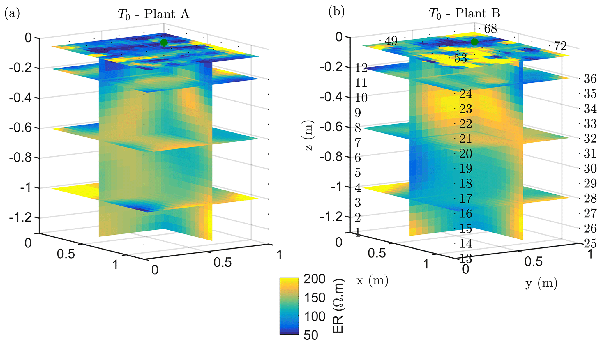
Figure 3Results of the 3D ERT inversion for the background time T0 for plant A (a) and B (b). Three-dimensional resistivity volume (log scale) sliced at the tree stem position (vertically) and at four depths (0.05, 0.2 0.6 and 1 m), with the green point showing the location of the plant stem.
The T1 time step was collected during the irrigation, at 2 h for plant A and at 30 min for plant B after the beginning of the irrigation, so the variations of ER values are not directly comparable for the two plants. Figure 4a shows the resistivity distribution during irrigation (at time step T1) and after irrigation (T2 to T5) for plant B. The input of low resistivity water (13.88 Ωm, measured in laboratory) caused a homogeneous drop of the resistivity values (as much as 100 Ωm difference) around plant B. The observed resistivity decrease in the upper 40 cm can be attributed to the presence of a porous layer and correspondingly fast infiltration. A similar drop can be seen for plant A (Fig. B1). This is indirect evidence that water infiltrated both areas (that are next to each other) with no difference in soil hydraulic properties. For the time after irrigation, it is difficult to appreciate the change in resistivity from the absolute values, while time-lapse inversion (Fig. 4b) shows that the main increase in ER (up to 140 % of the background value) was located in the upper layers (< 0.3 m depth) and occurred between the background time and T3. Note that the acquisition time T3 corresponds to the morning of the following day, since no measurements were taken overnight, and the acquisition time matches with the start of the increase in ET and mean air temperature. No increase was observed on plant A (Fig. B1). After T3, no positive change in ER was observed.
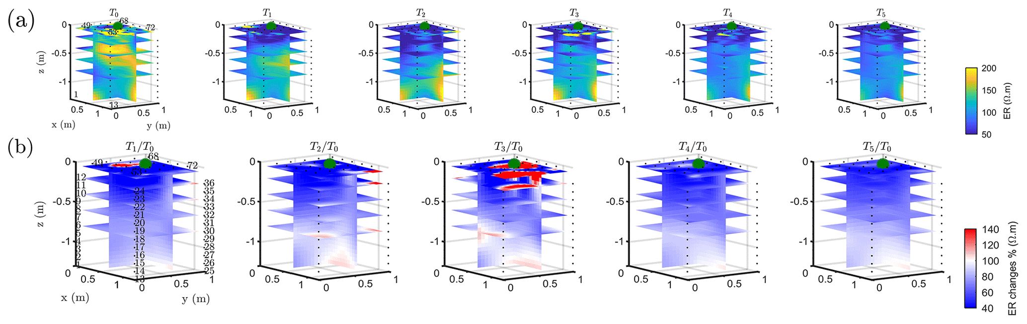
Figure 4Three-dimensional ERT results for plant B (plant A, in Appendix Fig. B1). The volume is sliced at the tree stem position (vertically) and at five depths (0.05, 0.2, 0,4, 0.6 and 0.8 m). (a) Three-dimensional inversion of the resistivity (in Ωm, log scale) from the background time T0, during irrigation T1 and after irrigation. (b) Time-lapse inversion (following Cassiani et al., 2006) showing the ratios (in % of ER changes) between time step Ti and background time T0 (100 % in white means no change).
3.2 Background and irrigation time steps of MALM-measured data
Figure 5 shows the raw results of MALM acquisition on plant B, during background and irrigation, for both soil and stem injection configurations. Note that voltages are normalized against the corresponding injected current. For both surface and borehole electrodes the normalized voltage distribution can be compared against the one expected from the solution for a single current electrode, idealized as a point injection of current I at the surface of a homogeneous soil of resistivity ρ:
where r is the distance between the (surface) injection point and the point where voltage V is computed (see Fig. 5e for a comparison). In all cases, both for surface and borehole electrodes, and both for stem and soil current injection, the resistance patterns are deformed with respect to the solution of Eq. (4) for a homogeneous soil. Some pieces of evidence are apparent from the following.
- a.
In all cases, the pattern of surface and subsurface resistance is asymmetric with respect to the injection point (in the stem or close to it, in the soil) and thus different from the predictions of Eq. (3); this indicates that current pathways are controlled by the soil heterogeneous structure: note that at all times there is a clear indication that a conductive pathway extends from the plant to the upper-right corner of the image (this would be the classical use of MALM – identifying the shape of conductive bodies underground). Note that spatial variations of resistance between boreholes are consistent with surface observations; i.e. the maximum resistance was measured on the fourth borehole, located in the top right corner of the plot.
- b.
The resistance patterns in the case of stem injection are clearly different from the corresponding ones obtained from soil injection. In particular, injecting in the soil directly produces a stronger resistance signal both at the surface and in the boreholes than the corresponding resistance in the case of stem injection: this difference clearly points towards the fact that the plant root system must convey the current in a different way than the soil alone; tentatively the observed resistance features would indicate a deeper current injection in the case of stem injection. Looking at the qualitative differences between soil and stem injection in the borehole electrode data, the impact is very small at depths larger than 0.6 m.
- c.
For both soil and stem injection, local anomalies observed in the background image are either removed or smoothed during the irrigation steps. The effect is equally pronounced in soil and stem injection, showing that this is caused essentially by the change in resistivity induced by the change in soil water content (see Fig. 5).
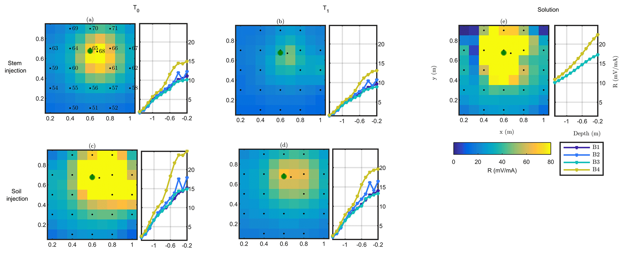
Figure 5Plant B MALM results showing variations in surface (horizontal plan) of resistance R (in mV mA−1) for the initial state background T0 (a, c) and irrigation T1 (b, d) time steps. Comparison between the stem injection (a, b) and soil injection (c, d). The black points show the surface electrode location. The green point shows the positions of the plant stem. Data are filtered using a threshold on reciprocal acquisition of 20 %. Panel (e) shows the solution using Eq. (4) for a homogeneous soil of 100Ωm; the resistances between boreholes B1/B3 and B2/B4 (see legend) are identical and cannot be distinguished graphically in the case of (e).
Similar features are observed for plant A (results shown in Appendices C1 and C2). The full-time monitoring is also shown only in Appendix C since a consistent and quantitative interpretation is not straightforward by a visual inspection of the raw MALM data.
3.3 Inversion of virtual current sources to estimate root extents
Figure 6 shows the iso-surfaces of the fitness index (or misfit) F1 (Eq. 2) for the background (pre-irrigation) conditions of plant B (plant A in Appendix C3) and for current injection in the soil and in the stem at all time steps listed in Table 1. In all cases, Fig. 6 shows the iso-surface corresponding to the value F1=7 V corresponding to the 25 % misfit index (value selected after analysing the evolution of the L curve of sorted misfit F1). The same threshold is fixed for all the time steps; thus, the images provide comparable information for all cases. Note, nevertheless, that the position of the active roots from one acquisition to the other during the irrigation experiment (or for different seasons) may vary, which consequently affects the distribution of the misfit and ultimately the depth of the iso-surface describing active roots.
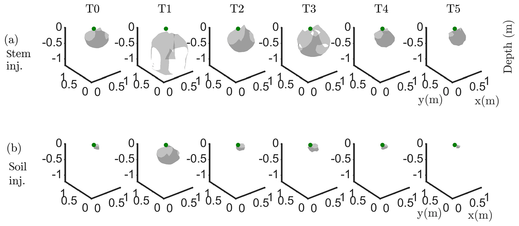
Figure 6Iso-surface minimizing the F1 function for plant B: during stem injection (a) and during soil injection (b). Columns represent the six time steps from T0 to T5. Green dot shows plant stem position. Threshold is defined by the misfit 25 % of the normalized F1 (value selected according to the evolution of the curve of sorted misfit F1, calculated for the tree injection at T0 and kept constant for all the time steps).
In particular, the F1 procedure highlights the remarkable difference, for both plants A and B, between the injection in the stem and in the soil. Current injection in the soil produces a voltage distribution that, albeit corresponding to a heterogeneous resistivity distribution and thus different from the predictions of a simpler model such as Eq. (3), collapses effectively to one point, i.e. the point where current was effectively injected into the ground. On the contrary, when current is injected into the stem, the region of possible source locations in the ground is much wider and depicts a volume that is likely to correspond to the contact points between roots and soil, i.e. the volume where roots have an active role in the soil especially in terms of RWU. While this latter interpretation remains somewhat speculative, at least in the present experimental context, the different results between soil and stem injection can only find an explanation in the role of roots and their spatial structure.
The most interesting feature shown by Fig. 6 is that the likely source volumes do not change with time during irrigation except for the irrigation time T1 for which the iso-surface extended slightly more at depth. Note that the F1 procedure makes use of the changing electrical resistivity distributions caused by infiltrating water (see Fig. 4); thus, the result is not obvious and indicates an underlying mechanism that is likely to be linked to the permanence of the root structure over such a short time span.
Figure 7 shows the spatial distribution of the current density as an outcome of the minimization of the F2 function. Very similar observations to F1 are driven from the current source density, i.e. that current injection in the soil produces a current distribution that collapses effectively to one point, which is the point where current was effectively injected into the ground, while when current is injected into the stem, the current distribution in the ground is much wider and depicts a volume that is likely to correspond to the contact points between roots and soil. Note that the different time steps (Fig. C4) did not highlight changes in the distribution of current density, suggesting that the region of RWU was relatively constant during the experiment.

Figure 7Current source density after minimization of the objective function F2 as defined in Eq. (3). The results are relevant to the background time T0 for plant B, for the soil current injection (a) and the stem current injection (b).
3.4 Electrical resistivity variations inside and outside the likely active root zone
Our assumption is that the region identified by MALM F1 for the background time corresponds to the RWU region. The inner area (IN) is then defined as the area within the closed iso-surface at the background time T0. As the changes in the estimated extent of the root zone are only minor (Fig. 6), it makes sense to evaluate the changes, as an effect of irrigation, in electrical resistivity within such a stable estimated root zone. Figure 8 shows the ER variations of selected values in the zones outside and inside this estimated active root zone. It is apparent how irrigation causes a general decrease in electrical resistivity for both plants A (Fig. 8a) and B (Fig. 8b) and in both the inner and outer regions. Note that, even though the regions are different for the two plants, the behaviour is similar. Then at the end of irrigation we observe, for both plants, that resistivity continues to decrease outside the root-active region, while it increases slightly inside. This behaviour is consistent with the fact that inside the region we expect that RWU progressively dries the soil, while outside this region resistivity continues to decrease (overall) as an effect (probably) of water redistribution in the unsaturated soil.
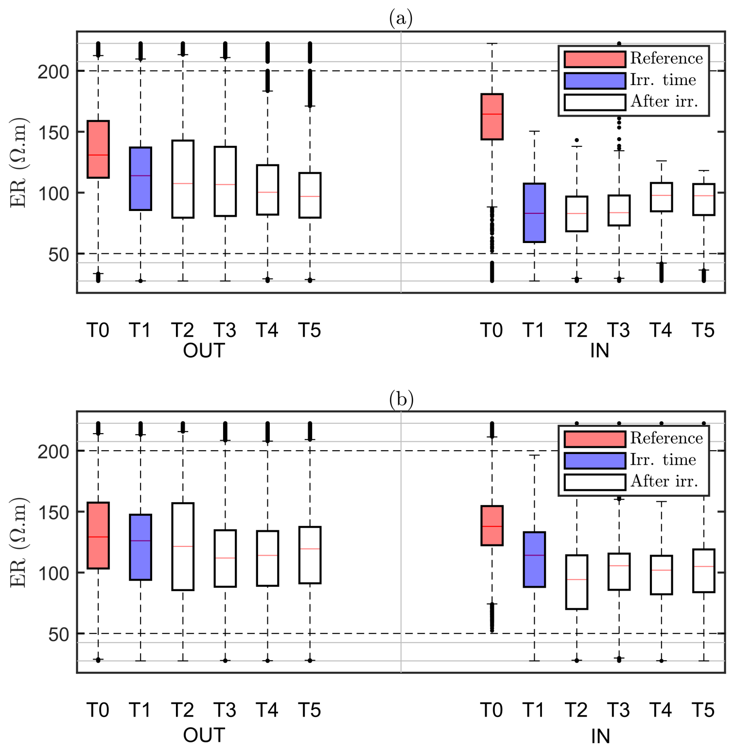
Figure 8Boxplot distribution of ER time variations observed on plant A (a) and plant B (b) for the values selected outside (OUT, left part) and inside (IN, right part) of the region defined by the F1 best-fit sources (see Fig. 6a – T0). The central mark indicates the median; the bottom and top edges of the box indicate the 25th and 75th percentiles of the ER data, respectively. The whiskers extend to the most extreme data points (black dots) considered outliers. Each box corresponds to a given time step (see Table 1), indicated in the x axis.
3.5 One-dimensional simulation of the infiltration
Figure 9a shows the variations of the simulated soil water content (θsimu) with time for control points located at different depths (see Fig. 2 for the geometry), and Fig. 9b shows the comparison against the three-dimensional variations of ER transformed values to soil water content (θERT). Time steps of the ERT acquisition for starting time and end time are reported on Fig. 9a for an easier comparison with Fig. 9b. At T0, values of soil water content are about 0.1, a value close to field capacity for this type of soil, as previously assumed (Sect. 2.2) and in agreement with the literature. Despite all the assumptions and models' limitation described later, the range of soil water seems also consistent between the simulation and the measured data. Note also that the dynamic is closely linked to the estimated ET and mean air temperature shown in Fig. 2. The start and end time of the triggered irrigation are clearly identified respectively with a sharp increase followed by a decrease in θsimu at z=0, with a peak in SWC equal to 0.3. Between T1 and T2, only the upper surface (< 0.2 m depth) is affected by the irrigation front resulting in the increase in soil water content visible in both θsimu and θERT (Fig. 9b). The infiltration front reaches the depth of 0.4 m during the collection of ERT data at time T2. Time T2 marks the start of a regular decrease in the soil water content overnight in the top 40 cm soil. Time T3, coincident with an increasing ET and mean air temperature, highlights a rupture from a slow decrease to a higher decrease rate particularly for the soil surface (the layer < 0.2 m depth), in agreement with the observed changes in θERT (Fig. 9b). Overall, Fig. 9a and b show a good correlation between the dynamics of SWC changes predicted by the hydrological model (θsimu) and observed via the ER transformed values (θERT).
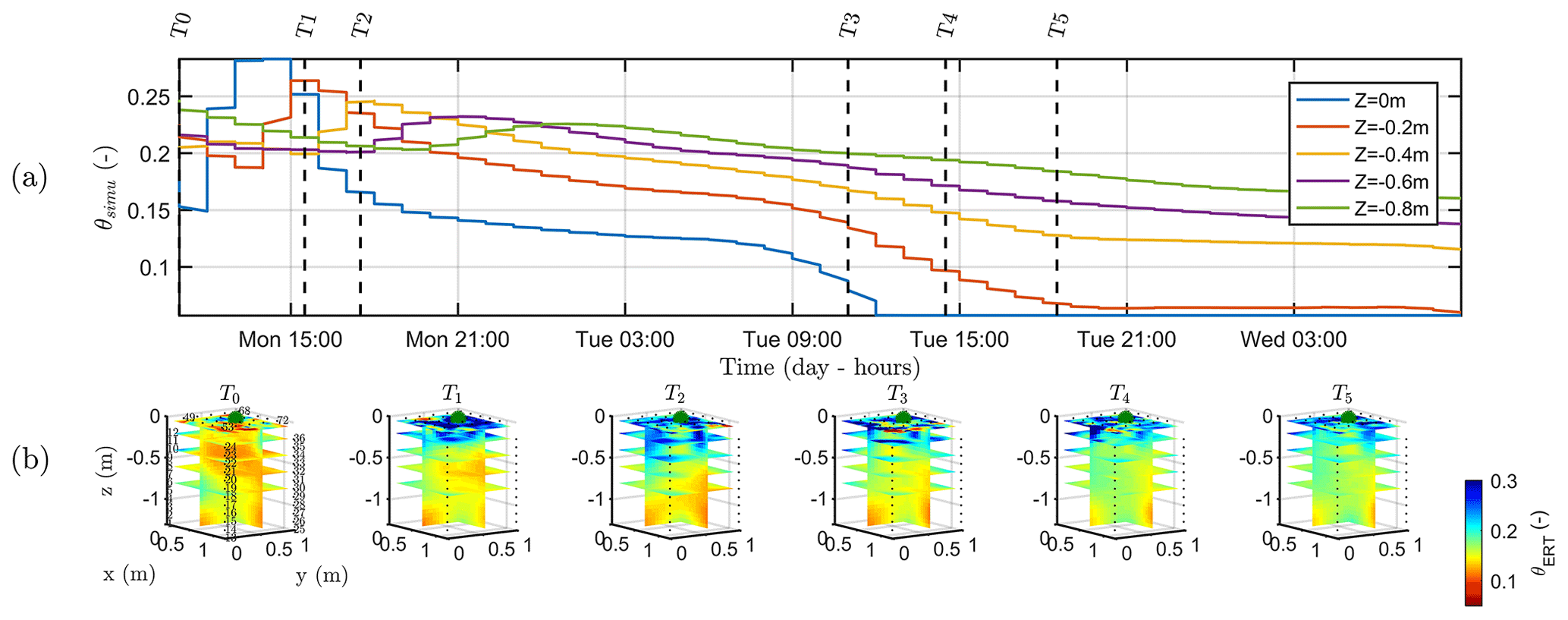
Figure 9(a) Time variation of simulated soil water content (θsimu) at five depths. The vertical lines indicate the geophysical acquisition times (dashed and plain line respectively for the start and the end of the measurement; see Table 1). (b) Three-dimensional variations of the ERT-derived soil water content (θERT) for the time steps described in Table 1. Horizontal layer depths are identical to the control points of the hydrological model.
The survey was carried out during a sunny summer season in a non-irrigated vineyard of the Bordeaux region. The site is composed of sandy loam soil; thus, there is a high infiltration rate during the experiment, and this would make it more difficult to distinguish RWU zones from infiltration zones as done for instance by Cassiani et al. (2015) using time-lapse ERT alone.
The first objective of the study was to define a non-invasive investigation protocol capable of imaging the root activity as well as the distribution of active roots under varying soil water content. We demonstrated that the key additional information is provided by MALM, which directly incorporates the ERT information in terms of changing electrical resistivity distribution in space including its evolution in time. MALM, and particularly its double application of current injection in the stem and in the soil next to it, uses electrical measurements in a totally different manner: here the plant root system itself acts as a conductor, and the goal is to use the retrieved voltage distribution to infer where the current injected into the stem actually is conveyed into the soil: these locations are potentially the same locations where roots interact with the soil in terms of RWU. However, in order to try and locate the position of these points, it is necessary to know the soil electrical resistivity distribution at the time of measurements. At this scale of measurements, ERT provides 3D images of electrical resistivity distribution in the subsoil housing the root system. Fast acquisition allows the measurement of resistivity changes over time, which in turn can be linked to changes in SWC. This can be caused for example by water infiltration or by RWU: in the latter case, negative SWC changes mapped through resistivity changes can be used to map the regions where roots exert an active suction and reduce SWC. However, water redistribution in the soil also plays a role in terms of resistivity changes. Thus some additional independent information about the location of active roots in the soil may help: this is the first coupling between ERT and MALM that has been integrated in the workflow. Considering the inverted MALM data as non-sensitive to soil water distribution has different potential useful impacts: the separation of contributions of the root zone and outer area on ER values extracted from ERT help distinguish between soil processes such as RWU and hydraulic redistribution (hydraulic lift in particular).
Time-lapse ERT measurements give clear evidence that injecting current into the stem and into the soil close to the stem produces different inversions even under changing soil water conditions. The soil injection produces a current density close to a punctual injection (located at the true single-electrode location) regardless of the soil water content. The stem injection helps identify a 3D region of likely distributed current injection locations, thus defining a region in the subsoil where RWU is likely to take place. The latter result is particularly useful, in perspective: when computing the time-lapse changes of electrical resistivity inside and outside this tentative RWU region during irrigation we clearly see that while inside resistivity increases (as an effect of RWU, as irrigation is still ongoing), outside resistivity decreases. Thus, our assumption that the region identified by MALM inversion (albeit very rough) corresponds to the RWU region is corroborated indirectly also by this evidence.
4.1 Comparison between geophysical data and hydrological model
A second objective of the study was to integrate the geophysical results in a simple 1D model of the infiltration experiment that takes into account the observed water fluxes. Dupuy et al. (2010) advocated the use of root systems described as density distributions. We assimilated the root distribution, derived from the geophysical data, into the hydrological model. Attempts in this direction are very promising to describe the root functioning in the framework of continuum physics, i.e. the one endorsed by SPAC. The integration of modelling and data has proven a key component of this type of hydro-geophysical studies, allowing us to draw quantitative results of practical interest. For example, in our study it is apparent that although infiltration occurred during the peak of evapotranspiration (between 01:00 and 03:00 pm), very low RWU was observed before the second day. Nevertheless, after a certain time, RWU is observed while infiltration is still ongoing. Smaller RWU observed for the small plant A compared to plant B is also observed.
4.2 Recommendation for future experiments
In this field case study, we had very little available quantitative information that could allow the validation of the geophysical data in terms of the volume of soil affected by RWU. The final objective of this study was then to discuss issues for obtaining suitable validation data using existing methods and propose some recommendation for future experiments.
- i.
Traditional root sampling methods should be the first line of validation although they have numerous potential pitfalls. As roots are underground, and thus invisible in their space–time evolution, and are also fragile, especially in their fine structure, the monitoring of their structure and activity using destructive methods such as trenches or air spade presents various limitations. In such approaches, even in the best case where fine roots may be sufficiently preserved and described, it is impossible to know where the active roots actually are. Active roots may be located only in one part of the whole root system. Destructive methods may help to validate the confidence area determined by F1 but are not appropriate methods to validate the F2 inversion.
- ii.
We recommend the use of traditional methods (such as TDR and tensiometers) for future studies. Though punctual, these data can greatly facilitate the data calibration and validation of geophysical methods.
Finally, more research needs to be conducted to understand how MALM can provide information to be correlated with the actual RWU and thus to the estimated transpiration. The study of complex root–soil interactions requires that high-time-resolution and extensive data are collected and processed. In order to quantitatively evaluate RWU using the variations of ER, many more data instances per day must be acquired. In this study, we only used ERT and MALM information to initialize the infiltration model, and only a qualitative comparison was conducted between model predictions and geophysical results. In the near future, a real assimilation scheme using the data assimilation technique should be adopted.
This study presents an approach to define the extent of active root distribution using non-invasive investigations and is thus particularly suitable to be applied under real field conditions. We applied a mix of ERT and MALM techniques, using the same electrode and surface electrode distribution. The power of the approach lies in the complementary capabilities of the two techniques in providing information concerning the root structure and activity. The approach has been tested in a vineyard during an irrigation experiment. Future experiments would require that high-time-resolution and extensive data are collected and that the results are analysed in conjunction with data from traditional monitoring methods in order to qualitatively integrate geophysical results into a hydrological one. The presented approach can be easily replicated under a variety of conditions, as DC electrical methods such as ERT and MALM do not possess a spatial scaling per se, but their resolution depends on electrode spacing as well as on other factors that are difficult to assess a priori, such as resistivity contrasts and signal-to-noise ratio. Thus similar experiments can also be used in the laboratory, where more direct evidence of root distribution can be used to further validate the method.

Figure A1(a–c) Three-dimensional view of the surface (blue) and borehole (black) electrodes; view from the top and transversal view. Plant A was located downhill. Green dot shows plant stem positions.
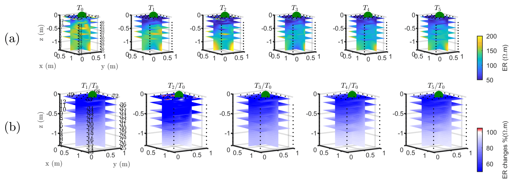
Figure B1Three-dimensional ERT results for plant A. The volume is sliced at the tree stem position (vertically) and at five depths (0.05, 0.2, 0,4, 0.6 and 0.8 m). (a) Three-dimensional inversion of the resistivity (in Ωm, log scale) from the background time T0, during irrigation T1 and after irrigation. (b) Time-lapse inversion (following Cassiani et al., 2006) showing the ratios (in % of ER changes) between time step Ti and background time T0 (100 % in white means no change).
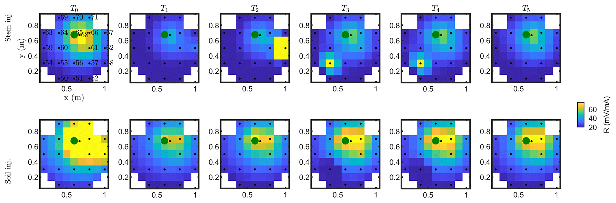
Figure C1Resistance distribution of the raw data of MALM time-lapse monitoring for plant B. First-line results are relevant to the stem injection, while the second line refers to the soil control injection. Columns describe time evolution according to Table 1.
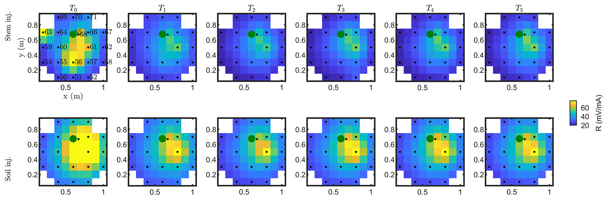
Figure C2Resistance distribution of the raw data of MALM time-lapse monitoring for plant A. First-line results are relevant to the stem injection, while the second line refers to the soil control injection. Columns describe time evolution according to Table 1.
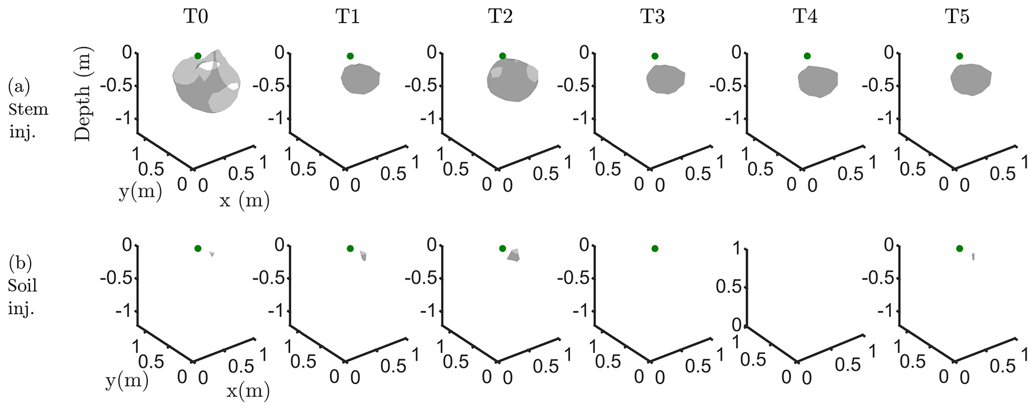
Figure C3Iso-surface minimizing the F1 function for plant A: during stem injection (a) and during soil injection (b). Columns represent the six time steps from T0 to T5. Green dot shows plant stem position. Threshold is defined by the misfit 25 % of the normalized F1 (value selected according to the evolution of the curve of sorted misfit F1, calculated for the tree injection at T0 and kept constant for all the time steps).

Figure C4Time-lapse evolution of the current source density after minimization of the objective function F2 as defined in Eq. (3). The results are relevant to the background time T0 to T5 for plant B, for the soil current injection on the left and stem current injection on the right.
Data used to generate the figures can be accessed on the Padua Research Archive (http://researchdata.cab.unipd.it/id/eprint/321 (Mary, 2020). ).
GC, YW and SSH worked on the conceptualization of the research. BM curated the data. LP, BM, NC and JB collected the data. BM prepared the formal analysis, designed and wrote the scripts for carrying out the simulation and inversion, and ran the obtained the results. MS and GC supervised the field work. All the authors discussed the results. BM prepared the paper with contributions from all the authors.
The authors declare that they have no conflict of interest.
The authors wish to acknowledge support from the ERANETMED (grant no. FP7) project WASA (“Water Saving in Agriculture: Technological developments for the sustainable management of limited water resources in the Mediterranean area”). Benjamin Mary gratefully acknowledge the University of Padua for the funding of the “Assegno di ricerca”. In addition, the information, data and work presented herein was funded in part by the Department of Energy Advanced Research Projects Agency-Energy (ARPA-E) project under work authorization no. 16/CJ000/04/08 and an Office of Science Biological and Environmental Research Watershed Function SFA project under contract no. DE-AC02-05CH11231. The views and opinions of authors expressed herein do not necessarily state or reflect those of the United States Government or any agency thereof. Luca Peruzzo and Myriam Schmutz gratefully acknowledge the financial support from IDEX (Initiative D’EXellence, France).
This research has been supported by the ERANETMED (grant no. FP7), the Hydro-geophysical monitoring and modelling for the Earth's Critical Zone (grant no. CPDA147114), and the European Union's Horizon 2020 research and innovation programme under a Marie Sklodowska-Curie grant agreement (grant no. 842922).
This paper was edited by Paul Hallett and reviewed by three anonymous referees.
Amato, M., Bitella, G., Rossi, R., Gómez, J. A., Lovelli, S., and Gomes, J. J. F.: Multi-electrode 3D resistivity imaging of alfalfa root zone, Eur. J. Agron., 31, 213–222, https://doi.org/10.1016/j.eja.2009.08.005, 2009.
Anderegg, W. R. L., Kane, J. M., and Anderegg, L. D. L.: Consequences of widespread tree mortality triggered by drought and temperature stress, Nat. Clim. Change, 3, 30–36, https://doi.org/10.1038/nclimate1635, 2013.
Archie, G. E.: The Electrical Resistivity Log as an Aid in Determining Some Reservoir Characteristics, Transactions of the AIME, 146, 54–62, https://doi.org/10.2118/942054-G, 1942.
Band, L. E., McDonnell, J. J., Duncan, J. M., Barros, A., Bejan, A., Burt, T., Dietrich, W. E., Emanuel, R., Hwang, T., Katul, G., Kim, Y., McGlynn, B., Miles, B., Porporato, A., Scaife, C., and Troch, P. A.: Ecohydrological flow networks in the subsurface, Ecohydrol., 7, 1073–1078, https://doi.org/10.1002/eco.1525, 2014.
Blanchy, G., Saneiyan, S., Boyd, J., McLachlan, P., and Binley, A.: ResIPy, an intuitive open source software for complex geoelectrical inversion/modeling, Comput. Geosci., 137, 104423, https://doi.org/10.1016/j.cageo.2020.104423, 2020.
Binley, A. and Kemna, A.: DC resistivity and induced polarization methods, in: Hydrogeophysics, Springer, 129–156, 2005.
Brovelli, A. And Cassiani, G.: Combined estimation of effective electrical conductivity and permittivity for soil monitoring: electrical conductivity and permittivity of soils, Water Resour. Res., 47, https://doi.org/10.1029/2011WR010487, 2011.
Brillante, L., Mathieu, O., Bois, B., van Leeuwen, C., and Lévêque, J.: The use of soil electrical resistivity to monitor plant and soil water relationships in vineyards, SOIL, 1, 273–286, https://doi.org/10.5194/soil-1-273-2015, 2015.
Campbell, R. B., Bower, C. A., and Richards, L. A.: change of electrical conductivity with temperature and the relation of osmotic pressure to electrical conductivity and ion concentration for soil extracts, Soil Sci. Soc. Am. J., 13, 66–69, https://doi.org/10.2136/sssaj1949.036159950013000C0010x, 1949.
Cassiani, G., Bruno, V., Villa, A., Fusi, N., and Binley, A. M.: A saline trace test monitored via time-lapse surface electrical resistivity tomography, J. Appl. Geophys., 59, 244–259, https://doi.org/10.1016/j.jappgeo.2005.10.007, 2006.
Cassiani, G., Ursino, N., Deiana, R., Vignoli, G., Boaga, J., Rossi, M., Perri, M. T., Blaschek, M., Duttmann, R., Meyer, S., Ludwig, R., Soddu, A., Dietrich, P., and Werban, U.: Noninvasive Monitoring of Soil Static Characteristics and Dynamic States: A Case Study Highlighting Vegetation Effects on Agricultural Land, Vadose Zone J., 11, vzj2011.0195, https://doi.org/10.2136/vzj2011.0195, 2012.
Cassiani, G., Boaga, J., Vanella, D., Perri, M. T., and Consoli, S.: Monitoring and modelling of soil–plant interactions: the joint use of ERT, sap flow and eddy covariance data to characterize the volume of an orange tree root zone, Hydrol. Earth Syst. Sci., 19, 2213–2225, https://doi.org/10.5194/hess-19-2213-2015, 2015.
Cassiani, G., Boaga, J., Rossi, M., Putti, M., Fadda, G., Majone, B., and Bellin, A.: Soil–plant interaction monitoring: Small scale example of an apple orchard in Trentino, North-Eastern Italy, Sci. Total Environ., 543, 851–861, https://doi.org/10.1016/j.scitotenv.2015.03.113, 2016.
Chahine, M. T.: The hydrological cycle and its influence on climate, Nature, 359, 373–380, https://doi.org/10.1038/359373a0, 1992.
Consoli, S., Stagno, F., Vanella, D., Boaga, J., Cassiani, G., and Roccuzzo, G.: Partial root-zone drying irrigation in orange orchards: Effects on water use and crop production characteristics, Eur. J. Agron., 82, 190–202, https://doi.org/10.1016/j.eja.2016.11.001, 2017.
Couvreur, V., Vanderborght, J., and Javaux, M.: A simple three-dimensional macroscopic root water uptake model based on the hydraulic architecture approach, Hydrol. Earth Syst. Sci., 16, 2957–2971, https://doi.org/10.5194/hess-16-2957-2012, 2012.
Dalton, F. N.: In-situ root extent measurements by electrical capacitance methods, Plant Soil, 173, 157–165, https://doi.org/10.1007/BF00155527, 1995.
Dawson, T. E. and Siegwolf, R. T. W. (Eds.): Stable isotopes as indicators of ecological change, 1st Edn., Academic, Oxford, 2007.
de Arellano, J. V.-G., van Heerwaarden, C. C., and Lelieveld, J.: Modelled suppression of boundary-layer clouds by plants in a CO2-rich atmosphere, Nat. Geosci., 5, 701–704, https://doi.org/10.1038/ngeo1554, 2012.
De Carlo, L., Perri, M. T., Caputo, M. C., Deiana, R., Vurro, M., and Cassiani, G.: Characterization of a dismissed landfill via electrical resistivity tomography and mise-à-la-masse method, J. Appl. Geophys., 98, 1–10, https://doi.org/10.1016/j.jappgeo.2013.07.010, 2013.
Dirmeyer, P. A., Koster, R. D., and Guo, Z.: Do Global Models Properly Represent the Feedback between Land and Atmosphere?, J. Hydrometeor., 7, 1177–1198, https://doi.org/10.1175/JHM532.1, 2006.
Dirmeyer, P. A., Jin, E. K., Kinter III, J. L., and Shukla, J.: Land Surface Modeling in Support of Numerical Weather Prediction and Sub-Seasonal Climate Prediction, White Paper: Workshop on Land Surface Modeling in Support of NWP and Sub-Seasonal Climate Prediction, 17 pp., 2014.
Draye, X., Kim, Y., Lobet, G., and Javaux, M.: Model-assisted integration of physiological and environmental constraints affecting the dynamic and spatial patterns of root water uptake from soils, J. Exp. Bot., 61, 2145–2155, https://doi.org/10.1093/jxb/erq077, 2010.
Dupuy, L., Fourcaud, T., Stokes, A., and Danjon, F.: A density-based approach for the modelling of root architecture: application to Maritime pine (Pinus pinaster Ait.) root systems, J. Theor. Biol., 236, 323–334, https://doi.org/10.1016/j.jtbi.2005.03.013, 2005.
Dupuy, L., Vignes, M., Mckenzie, B. M., and White, P. J.: The dynamics of root meristem distribution in the soil, Plant Cell Environ., 33, 358–369, https://doi.org/10.1111/j.1365-3040.2009.02081.x, 2010.
Dupuy, L. X. and Vignes, M.: An algorithm for the simulation of the growth of root systems on deformable domains, J. Theor. Biol., 310, 164–174, https://doi.org/10.1016/j.jtbi.2012.06.025, 2012.
Feddes, R. A., Kowalik, P. J., and Zaradny, H.: Simulation of field water use and crop yield. Simulation monographs, Pudoc, Wageningen, 9–30, 1978.
Garré, S., Javaux, M., Vanderborght, J., Pagès, L., and Vereecken, H.: Three-Dimensional Electrical Resistivity Tomography to Monitor Root Zone Water Dynamics, Vadose Zone J., 10, 412–424, https://doi.org/10.2136/vzj2010.0079, 2011.
Gerwitz, A. and Page, E. R.: An Empirical Mathematical Model to Describe Plant Root Systems, J. Appl. Ecol., 11, 773, https://doi.org/10.2307/2402227, 1974.
Gibert, D., Le Mouël, J.-L., Lambs, L., Nicollin, F., and Perrier, F.: Sap flow and daily electric potential variations in a tree trunk, Plant Sci., 171, 572–584, https://doi.org/10.1016/j.plantsci.2006.06.012, 2006.
Hackett, C. and Rose, D.: A Model of the Extension and Branching of a Seminal Root of Barley, and Its Use in Studying Relations Between Root Dimensions I. the Model, Aust. J. Biol. Sci., 25, 669–680, https://doi.org/10.1071/BI9720669, 1972.
Jourdan C. and H. Rey:, Modelling and simulation of the architecture and development of the oil-palm (Elaeis guineensis Jacq) root system, 1. The model, Plant Soil, 190, 217–233, https://doi.org/10.1023/A:1004218030608, 1997.
Kemna, A., Binley, A., Cassiani, G., Niederleithinger, E., Revil, A., Slater, L., Williams, K. H., Orozco, A. F., Haegel, F.-H., Hördt, A., Kruschwitz, S., Leroux, V., Titov, K., and Zimmermann, E.: An overview of the spectral induced polarization method for near-surface applications, Near Surf. Geophys., 10, 453–468, https://doi.org/10.3997/1873-0604.2012027, 2012.
Mary, B., Saracco, G., Peyras, L., Vennetier, M., Mériaux, P., and Camerlynck, C.: Mapping tree root system in dikes using induced polarization: Focus on the influence of soil water content, J. Appl. Geophys., 135, 387–396, https://doi.org/10.1016/j.jappgeo.2016.05.005, 2016.
Mary, B., Abdulsamad, F., Saracco, G., Peyras, L., Vennetier, M., Mériaux, P., and Camerlynck, C.: Improvement of coarse root detection using time and frequency induced polarization: from laboratory to field experiments, Plant Soil, 417, 243–259, https://doi.org/10.1007/s11104-017-3255-4, 2017.
Mary, B., Peruzzo, L., Boaga, J., Schmutz, M., Wu, Y., Hubbard, S. S., and Cassiani, G.: Small-scale characterization of vine plant root water uptake via 3-D electrical resistivity tomography and mise-à-la-masse method, Hydrol. Earth Syst. Sci., 22, 5427–5444, https://doi.org/10.5194/hess-22-5427-2018, 2018.
Mary, B., Vanella, D., Consoli, S., and Cassiani, G.: Assessing the extent of citrus trees root apparatus under deficit irrigation via multi-method geo-electrical imaging, Sci. Rep., 9, 9913, https://doi.org/10.1038/s41598-019-46107-w, 2019.
Manoli, G., Bonetti, S., Domec, J.-C., Putti, M., Katul, G., and Marani, M.: Tree root systems competing for soil moisture in a 3D soil–plant model, Adv. Water Resour., 66, 32–42, https://doi.org/10.1016/j.advwatres.2014.01.006, 2014.
Mary, B.: Open data access to reproduce figures from the Soil Manuscript, available at: http://researchdata.cab.unipd.it/id/eprint/321, last access: 3 February 2020.
Maxwell, R. M., Chow, F. K., and Kollet, S. J.: The groundwater–land-surface–atmosphere connection: Soil moisture effects on the atmospheric boundary layer in fully-coupled simulations, Adv. Water Resour., 30, 2447–2466, https://doi.org/10.1016/j.advwatres.2007.05.018, 2007.
Michot, D., Benderitter, Y., Dorigny, A., Nicoullaud, B., King, D., and Tabbagh, A.: Spatial and temporal monitoring of soil water content with an irrigated corn crop cover using surface electrical resistivity tomography: soil water study using electrical resistivity, Water Resour. Res., 39, 1138–1158, https://doi.org/10.1029/2002WR001581, 2003.
Michot, D., Thomas, Z., and Adam, I.: Nonstationarity of the electrical resistivity and soil moisture relationship in a heterogeneous soil system: a case study, SOIL, 2, 241–255, https://doi.org/10.5194/soil-2-241-2016, 2016.
Mualem, Y.: A new model for predicting the hydraulic conductivity of unsaturated porous media, Water Resour. Res., 12, 513–522, https://doi.org/10.1029/WR012i003p00513, 1976.
Mualem, Y. and Friedman, S. P.: Theoretical Prediction of Electrical Conductivity in Saturated and Unsaturated Soil, Water Resour. Res., 27, 2771–2777, https://doi.org/10.1029/91WR01095, 1991.
Newman, B. D., Wilcox, B. P., Archer, S. R., Breshears, D. D., Dahm, C. N., Duffy, C. J., McDowell, N. G., Phillips, F. M., Scanlon, B. R., and Vivoni, E. R.: Ecohydrology of water-limited environments: A scientific vision: OPINION, Water Resour. Res., 42, https://doi.org/10.1029/2005WR004141, 2006.
Osiensky, J. L.: Ground water modeling of mise-a-la-masse delineation of contaminated ground water plumes, J. Hydrol., 197, 146–165, https://doi.org/10.1016/S0022-1694(96)03279-9, 1997.
Parasnis, D. S.: three-dimensional electric mise-a-la-masse survey of an irregular lead-zinc-copper deposit in central sweden, Geophys. Prospect, 15, 407–437, https://doi.org/10.1111/j.1365-2478.1967.tb01796.x, 1967.
Perri, M. T., De Vita, P., Masciale, R., Portoghese, I., Chirico, G. B., and Cassiani, G.: Time-lapse Mise-á-la-Masse measurements and modeling for tracer test monitoring in a shallow aquifer, J. Hydrol., 561, 461–477, https://doi.org/10.1016/j.jhydrol.2017.11.013, 2018.
Peruzzo, L.: PhD Thesis manuscript, Approches géoélectriques pour l'étude du sol et d'interaction sol-racines, Bordeaux 3, available at: http://www.theses.fr/s141626, 2019.
Philip, J. R.: Plant Water Relations: Some Physical Aspects, Annu. Rev. Plant. Physiol., 17, 245–268, https://doi.org/10.1146/annurev.pp.17.060166.001333, 1966.
Rao, S., Meunier, F., Ehosioke, S., Lesparre, N., Kemna, A., Nguyen, F., Garré, S., and Javaux, M.: Impact of Maize Roots on Soil-Root Electrical Conductivity: A Simulation Study, Vadose Zone J., 18, 190037, https://doi.org/10.2136/vzj2019.04.0037, 2019.
Rhoades, J. D., Raats, P. A. C., and Prather, R. J.: Effects of Liquid-phase Electrical Conductivity, Water Content, and Surface Conductivity on Bulk Soil Electrical Conductivity, Soil Sci. Soc. Am. J., 40, 651–655, https://doi.org/10.2136/sssaj1976.03615995004000050017x, 1976.
Richter, D. D. and Mobley, M. L.: Monitoring Earth's Critical Zone, Science, 326, 1067–1068, https://doi.org/10.1126/science.1179117, 2009.
Schaap, M. G., Leij, F. J., and van Genuchten, M. Th.: Rosetta?: a computer program for estimating soil hydraulic parameters with hierarchical pedotransfer functions, J. Hydrol., 251, 163–176, https://doi.org/10.1016/S0022-1694(01)00466-8, 2001.
Simunek, J., Sejna, M., Van Genuchten, M. T., Šimůnek, J., Šejna, M., Jacques, D., and Sakai, M.: HYDRUS-1D. Simulating the one-dimensional movement of water, heat, and multiple solutes in variably-saturated media, version 2, 1998
Srayeddin, I. and Doussan, C.: Estimation of the spatial variability of root water uptake of maize and sorghum at the field scale by electrical resistivity tomography, Plant Soil, 319, 185–207, https://doi.org/10.1007/s11104-008-9860-5, 2009.
Vanella, D., Cassiani, G., Busato, L., Boaga, J., Barbagallo, S., Binley, A., and Consoli, S.: Use of small scale electrical resistivity tomography to identify soil-root interactions during deficit irrigation, J. Hydrol., 556, 310–324, https://doi.org/10.1016/j.jhydrol.2017.11.025, 2018.
van Genuchten, M. Th.: A Closed-form Equation for Predicting the Hydraulic Conductivity of Unsaturated Soils, Soil Sci. Soc. Am. J., 44, 892–898, https://doi.org/10.2136/sssaj1980.03615995004400050002x, 1980.
Volpe, V., Marani, M., Albertson, J. D., and Katul, G.: Root controls on water redistribution and carbon uptake in the soil–plant system under current and future climate, Adv. Water Resour., 60, 110–120, https://doi.org/10.1016/j.advwatres.2013.07.008, 2013.
Waxman, M. H. and Smits, L. J. M.: Electrical Conductivities in Oil-Bearing Shaly Sands, Soc. Petrol. Eng. J., 8, 107–122, https://doi.org/10.2118/1863-A, 1968.
Weigand, M. and Kemna, A.: Multi-frequency electrical impedance tomography as a non-invasive tool to characterize and monitor crop root systems, Biogeosciences, 14, 921–939, https://doi.org/10.5194/bg-14-921-2017, 2017.
Weigand, M. and Kemna, A.: Imaging and functional characterization of crop root systems using spectroscopic electrical impedance measurements, Plant Soil, 435, 201–224, https://doi.org/10.1007/s11104-018-3867-3, 2019.
Werban, U., Attia al Hagrey, S., and Rabbel, W.: Monitoring of root-zone water content in the laboratory by 2D geoelectrical tomography, J. Plant Nutr. Soil Sci., 171, 927–935, https://doi.org/10.1002/jpln.200700145, 2008.
York, L. M., Carminati, A., Mooney, S. J., Ritz, K., and Bennett, M. J.: The holistic rhizosphere: integrating zones, processes, and semantics in the soil influenced by roots, J. Exp. Bot., 67, 3629–3643, https://doi.org/10.1093/jxb/erw108, 2016.