Word embeddings for application in geosciences: development, evaluation, and examples of soil-related concepts

A large amount of descriptive information is available in geosciences. This information is usually considered subjective and ill-favoured compared with its numerical counterpart. Considering the advances in natural language processing and machine learning, it is possible to utilise descriptive information and encode it as dense vectors. These word embeddings, which encode information about a word and its linguistic relationships with other words, lay on a multidimensional space where angles and distances have a linguistic interpretation. We used 280 764 full-text scientific articles related to geosciences to train a domain-specific language model capable of generating such embeddings. To evaluate the quality of the numerical representations, we performed three intrinsic evaluations: the capacity to generate analogies, term relatedness compared with the opinion of a human subject, and categorisation of different groups of words. As this is the first attempt to evaluate word embedding for tasks in the geosciences domain, we created a test suite specific for geosciences. We compared our results with general domain embeddings commonly used in other disciplines. As expected, our domain-specific embeddings (GeoVec) outperformed general domain embeddings in all tasks, with an overall performance improvement of 107.9 %. We also presented an example were we successfully emulated part of a taxonomic analysis of soil profiles that was originally applied to soil numerical data, which would not be possible without the use of embeddings. The resulting embedding and test suite will be made available for other researchers to use and expand upon.

1 Introduction

Machine learning (ML) methods have been used in many fields of geosciences (Lary et al., 2016) to perform tasks such as the classification of satellite imagery (Maxwell et al., 2018), soil mapping (McBratney et al., 2003), mineral prospecting (Caté et al., 2017), and flood prediction (Mosavi et al., 2018). Owing to their capability to deal with complex non-linearities present in the data, ML usually outperforms more traditional methods in terms of predictive power. The application of ML in geosciences commonly prioritises numerical or categorical data over qualitative descriptions, which are usually considered subjective in nature (McBratney and Odeh, 1997). However, the resources that have been invested in collecting large amounts of descriptive information from pedological, geological, and other fields of geosciences must be taken into account. Neglecting descriptive data due to their inconsistency seems wasteful; however, natural language processing (NLP) techniques, which involve the manipulation and analysis of language (Jain et al., 2018), have rarely been applied in geosciences.

For soil sciences, NLP opens the possibility to use a broad range of new analyses. Some examples include general, discipline-wide methods such as automated content analysis (Nunez-Mir et al., 2016) or recommendation systems (Wang and Blei, 2011) which can take advantage of the current literature. More specific cases could take advantage of big archives of descriptive data, such as those reported by Arrouays et al. (2017). The authors mention examples such as the Netherlands with more than 327 000 auger descriptions covering agricultural, forest, and natural lands, or the north-central US with 47 364 pedon descriptions covering eight states.

Approaches to deal with descriptive data include the work of Fonseca et al. (2002), who proposed the use of ontologies to integrate different kinds of geographic information. At the University of Colorado, Chris Jenkins created a structured vocabulary for geomaterials (https://instaar.colorado.edu/~jenkinsc/dbseabed/resources/geomaterials/, last access: 12 July 2019) using lexical extraction (Miller, 1995), names decomposition (Peckham, 2014), and distributional semantics (Baroni et al., 2012) in order to characterise word terms for use in NLP and other applications. A different approach, perhaps closer to the preferred quantitative methods, is the use of dense word embeddings (vectors) which encode information about a word and its linguistic relationships with other words, positioning it on a multidimensional space. The latter is the focus of this study.

There are many general-purpose word embeddings trained on large corpora from social media or knowledge organisation archives such as Wikipedia (Pennington et al., 2014; Bojanowski et al., 2016). These embeddings have been proven to be useful in many tasks such as machine translation (Mikolov et al., 2013a), video description (Venugopalan et al., 2016), document summarisation (Goldstein et al., 2000), and spell checking (Pande, 2017). However, for field-specific tasks, many researchers agree that word embeddings trained on specialised corpora can more successfully capture the semantics of terms than those trained on general corpora (Jiang et al., 2015; Pakhomov et al., 2016; Roy et al., 2017; Nooralahzadeh et al., 2018; Wang et al., 2018).

As far as we are aware, this is the first attempt to develop and evaluate word embedding for the geosciences domain. This paper is structured as follows: first, we define what word embeddings are, explaining how they work and showing examples to help the reader understand some of their properties; second, we describe the text data used and the pre-processes required to train a language model and generate these word embeddings (GeoVec); third, we illustrate how a natural language model can be quantitatively evaluated and we present the first test dataset for the evaluation of word embeddings specifically developed for the geosciences domain; fourth, we present results of an intrinsic evaluation of our language model using our test dataset and we explore some of the characteristics of the multidimensional space and the linguistic relationships captured by the model using examples of soil-related concepts; and finally, we present a simple, illustrative example of how the embedding can be used in a downstream task.

2 Word embeddings

Word embeddings have been commonly used in many scientific disciplines, thanks to their application in statistics. For example, one-hot encodings (Fig. 1), also know as “dummy variables”, have been used in regression analysis since at least 1957 (Suits, 1957). In one-hot encoding, each word is represented by a vector of length equal to the number of classes or words, where each dimension represents a feature. The problem with this representation is that the resulting array is sparse (mostly zeros) and very large when using large corpora; in addition, it also presents the problem of poor estimation of the parameters of the less-common words (Turian et al., 2010). A solution for these problems is the use of unsupervised learning to induce dense, low-dimensional embeddings (Bengio, 2008). The resulting embeddings lie on a multidimensional space where angles and distances have a linguistic interpretation.

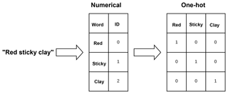
Figure 1 Example of two encodings of the phrase “red sticky clay”: numerical encoding and one-hot encoding.

These dense, real vectors allow models, specially neural networks, to generalise to new combinations of features beyond those seen during training due to the properties of the vector space where semantically related words are usually close to each other (LeCun et al., 2015). As the generated vector space also has properties such as addition and subtraction, Mikolov et al. (2013b) gives some examples of calculations that can be performed using word embedding. For instance the operation vec(“Berlin”) − vec(“Germany”) + vec(“France”) generates a new vector. When they calculated the distance from that resulting vector to all the words from the model vocabulary, the closest word was “Paris”. Fig. 2 presents a principal component analysis (PCA) projection of pairs of words with the country–capital relationship. Without explicitly enforcing this relationship when creating the language model, the resulting word embeddings encode the country–capital relationship due to the high co-occurrence of the terms. In Fig. 2 it is also possible to observe a second relationship, geographic location, where South American countries are positioned to the right, European countries in the middle, and (Eur-)Asian countries to the left.

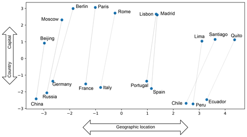
Figure 2 Examples of two-dimensional PCA projection of selected word embeddings using a general domain model. The figure illustrates the country–capital relationship learned by the model. Also notice that the model learned about the geographic relationship between the places. Example adapted from Mikolov et al. (2013b).

Potentially, each dimension and interaction within the generated vector space encodes a different type of relationship extracted from the data. Thanks to the properties of the generated vector space, we give ML algorithms the capacity to utilise and understand text, and we are able to use the same methods usually designed for numerical data (e.g. clustering, principal component). In the next sections, we describe how we generated a language model that yields word embeddings that encode semantic and syntactic relations specific for the geosciences domain, we visualise some of those relations, and we illustrate how to evaluate them numerically.

3 Data, text pre-processing, and model training

3.1 Corpus

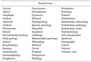
The corpus was generated by retrieving and processing 280 764 full-text articles related to geosciences. We used the Elsevier ScienceDirect APIs (application programming interfaces) to search for literature that matched the terms listed in Table 1, which cover a broad range of topics. These terms were selected based on their general relationship with geosciences and specifically soil science. We also included Wikipedia articles that list and concisely define some concepts such as types of rocks, minerals, and soils, providing more context than a scientific publication, considering that the model depends on words co-occurrences. We downloaded the text from Wikipedia articles “List_of_rock_types”, “List_of_minerals”, “List_of_landforms”, “Rock_(geology)”, “USDA_soil_taxonomy”, and “FAO_soil_classification”, and also all of the Wikipedia articles linked from those pages.

Table 1 Search terms used to retrieve full-text articles from Elsevier ScienceDirect APIs.

3.2 Pre-processing

The corpus was split into sentences which were then pre-processed using a sequence of commonly used procedures including the following:

1. removing punctuation,

2. lowercasing,

3. removing digits and symbols, and

4. removing (easily identifiable) references.

The cleaned sentences were then tokenised (split into words). In order to decrease the complexity of the vocabulary, we lemmatised all nouns to their singular form and removed all the words with less than three characters. We also removed common English words such as “the”, “an”, and “most” as they are not discriminating and unnecessarily increase the model size and processing time (a full list of the removed “stop words” can be found in the documentation of the NLTK Python library; Bird and Loper, 2004). Finally, we excluded sentences with less than three words. The final corpus has a vocabulary size of 701 415 (unique) words and 305 290 867 tokens.

3.3 Model training

For this work, we used the GloVe (Global Vectors) model (Pennington et al., 2014), developed by the Stanford University NLP group, which achieved great accuracy on word analogy tasks and outperformed other word embedding models on similarity and entity recognition tasks. As with many NLP methods, GloVe relays on ratios of word–word co-occurrence probabilities in the corpus. To calculate the co-occurrence probabilities, GloVe uses a local context window, where a pair of words d words apart contributes 1∕d to the total count. After the co-occurrence matrix X is calculated, GloVe minimises the least-squares problem

$$\begin{array}{}\text{(1)}& \sum _{i,j=\mathrm{1}}^{V}f\left(X_{ij}\right){\left({\mathit{w}}_i^T{\widehat{\mathit{w}}}_j+b_i+{\widehat{b}}_j-\log {\mathbf{X}}_{ij}\right)}^{\mathrm{2}},\end{array}$$

where X_ij is the co-occurrence between the target words i and the context word j, V is the vocabulary size, w_i is the word embedding, ${\widehat{\mathit{w}}}_j$ is a context word embedding, b_i and ${\widehat{b}}_j$ are biases for w_i and ${\widehat{\mathit{w}}}_j$, respectively, and f(X_ij) is the weighting function

$$\begin{array}{}\text{(2)}& f\left({\mathbf{X}}_{ij}\right)=\left\{\begin{array}{ll}({\mathbf{X}}_{ij}/x_{\text{max}}{)}^{\mathit{\alpha }}& \text{if}{\mathbf{X}}_{ij}<x_{\text{max}}\\ \mathrm{1}& \text{otherwise}\end{array}\right.\end{array}$$

that assures that rare and frequent co-occurrences are not overweighted. Pennington et al. (2014) recommend using the value 0.75 for the smoothing parameter α and the value 100 for the maximum cutoff count x_max.

We trained the model during 60 epochs, where 1 epoch corresponds to a complete pass through the training dataset. During the training phase, we experimented using embedding with different numbers of components (dimensions) and different context window sizes. Here we present the results for 300 components and a context window of size 10, which represents a good balance between model size, training time, and performance.

4 Evaluation of word embeddings

Given the characteristic of the vector space, the most common method to evaluate word embeddings is to assess their performance in tasks that test if semantic and syntactic rules are properly encoded. Many studies have presented datasets to perform this task. Rubenstein and Goodenough (1965) presented a set of 65 noun synonyms to test the relationship between the semantic similarity existing between a pair of words and the degree to which their contexts are similar. More recent and larger test datasets and task types have been proposed (Finkelstein et al., 2002; Mikolov et al., 2013c; Baroni et al., 2014), but they have all been designed to test general domain vectors. Because this work aims to generate embeddings for the geosciences domain, we developed a test suite to evaluate their intrinsic quality in different tasks, which are described below.

Analogy:

given two related pairs of words, a:b and x:y, the aim of the task is to answer the question “a is to x as b is to?”. The set includes 50 quartets of words with different levels of complexity, from simple semantic relationships to more advance syntactic relations. In practice, it is possible to find y by calculating the cosine similarity between the differences of the paired vectors:

$$\begin{array}{}\text{(3)}& {\displaystyle \frac{({\mathit{v}}_{\mathrm{b}}-{\mathit{v}}_{\mathrm{a}})\cdot ({\mathit{v}}_y-{\mathit{v}}_x)}{\Vert {\mathit{v}}_{\mathrm{b}}-{\mathit{v}}_{\mathrm{a}}\Vert \Vert {\mathit{v}}_y-{\mathit{v}}_x\Vert }}.\end{array}$$

In this case, v_y is the embedding for each word of the vocabulary and y is the word with the highest cosine similarity. Some examples of analogies are “moraine is to glacial as terrace is to []? (fluvial)”, “limestone is to sedimentary as tuff is to []? (volcanic)”, and “chalcanthite is to blue as malachite is to []? (green)”.

We estimated the top-1, top-3, top-5, and top-10 accuracy score, recording a positive result if y was within the first 1, 3, 5, or 10 words returned by the model, respectively.

Relatedness:

for a given pair of words (a,b), a score of zero or one is assigned by a human subject if the words are unrelated or related, respectively. The set includes 100 pairs of scored pairs of words. The scores are expected to have a high correlation with the cosine similarity between the embeddings of each pair of words. In this work, we used the Pearson correlation coefficient to evaluate the model against annotations made by three people with a geosciences background.

Categorisation:

given two sets of words $s_{\mathrm{1}}=\mathit{\{}a,b,c,\mathrm{\dots }\mathit{\}}$ and $s_{\mathrm{2}}=\mathit{\{}x,y,z,\mathrm{\dots }\mathit{\}}$, this test should be able to correctly assign each word to its corresponding group using a clustering algorithm. We provide 30 tests with 2 clusters each. We estimated the v-measure score (Rosenberg and Hirschberg, 2007), which takes the homogeneity and completeness of the clusters into account, after projecting the multidimensional vector space to a two-dimensional PCA space and performing a k-means clustering. Given that k-means is not deterministic (when using random centroids initiation), we used the mean v-measure score of 50 realisations.

We compared our results with general domain vectors trained on Wikipedia articles (until 2014) and the Gigaword v5 catalogue, which comprises 6 billion tokens and is provided by the authors of GloVe at https://nlp.stanford.edu/projects/glove/ (last access: 12 July 2019).

5 Illustrative example

In order to illustrate the use of word embedding in a downstream application, we decided to emulate part of the analysis of a soil taxonomic system performed by Hughes et al. (2017). They used 23 soil variables (e.g. sand content and bulk density), where the majority were numerical and continuous except for two binary variables representing the presence or absence of water or ice. Those variables correspond to the representation of horizons from soil profiles, which were then aggregated (mean) at different taxonomic levels to obtain class centroids.

Our analysis was similar, but, instead of using soil variables, we used the word embedding corresponding to the textual description of 10 000 soil profile descriptions downloaded from the United States Department of Agriculture–Natural Resources Conservation Service (USDA-NRCS) web site for official soil series descriptions and series classification. The descriptions were pre-processed utilising the same pipeline used for the corpus (Sect. 3.2). After obtaining the embeddings for each token in the descriptions, we calculated the mean values per profile, which can be considered as an embedding at the profile level. The profiles and their corresponding 300-dimensional embeddings were aggregated at the great group (GG) level (soil taxonomy) and a mean embedding value was estimated (equivalent to the centroids obtained by Hughes et al., 2017). After projecting the GG embeddings into a two-dimensional PCA space, we computed the convex-hull per soil order (smaller convex polygon needed to contain all the GG points for a particular soil order) as a way of visualising their extent.

6 Results and discussion

6.1 Co-occurrence

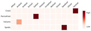
Before training the language model, the first output of the process is a co-occurrence matrix. This matrix encodes useful information about the underlying corpus (Heimerl and Gleicher, 2018). Figure 3 shows the co-occurrence probabilities of soil taxonomic orders and some selected words. It is possible to observe that concepts generally associated with a specific order co-occur in the corpus, such as the fact that soil cracks are features usually present in Vertisols, or that Andisols are closely related to areas with volcanic activity.

Figure 3 Co-occurrence probability matrix of soil orders (USDA) and selected words.

This information can also be used to guide the process of generating a domain-specific model. In our case, in an early stage of this study, the terms “permafrost” and “Gelisol” presented a very low co-occurrence probability, which was a clear sign of the limited topic coverage of the articles at that point.

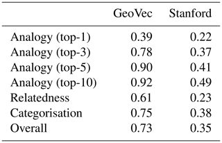
6.2 Intrinsic evaluation

The results of the intrinsic evaluation indicate that our domain-specific embeddings (GeoVec) performed better than the general domain embeddings in all tasks (Table 2), increasing the overall performance by 107.9 %. This is an expected outcome considering the specificity of the tasks. For the analogies, we decided to present the top-1, 3, 5, and 10 accuracy scores because, even if the most desirable result is to have the expected word as the first output from the model, in many cases the first few words are closely related or they are synonyms. For instance, for the analogy “fan is to fluvial as estuary is to []? (coastal)”, the first four alternatives are “tidal”, “river”, “estuarine”, and “coastal”, which are all related to a estuary.

In the relatedness task, the three human annotators had a high inter-annotator agreement (multi-kappa = 98.66 %; as per Davies and Fleiss, 1982), which was expected as the relations are not complex for someone with a background in geosciences. As we keep working on this topic, we plan to extend the test suite with more subtle relations.

Table 2 Evaluation scores for each task for our domain-specific (GeoVec) and general domain embeddings (Stanford). For the analogy task, top-1, 3, 5, and 10 represents the accuracy if the expected word was within the first 1, 3, 5, or 10 words returned by the model. For the relatedness task, the score represents the absolute value of the Pearson correlation (mean of the three human subjects). For the categorisation task, the score represents the mean value of 50 v-measure scores. The possible range of all scores is zero to one, where higher is better.

It was possible to observe an increase in the overall performance of the embeddings (calculated as the mean of the analogy – top-5, relatedness, and categorisation tasks) as we added more articles, almost stabilising around 300 million tokens, especially for the analogy task (Fig. 4). For domain-specific embeddings, this limit most likely varies depending on the task and domain. For instance, Pedersen et al. (2007), measuring semantic similarity and relatedness in the biomedical domain, found a limit of around 66 million tokens.

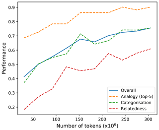
Figure 4 Overall performance of the embeddings versus number of tokens used to construct the co-occurrence matrix. The improvement limit is around 300 million tokens. For future comparisons, this limit corresponds to approximately 280 000 articles, 22.5 million sentences and 700 000 unique tokens.

The improvement over the general domain embeddings has also been reported in other studies. Wang et al. (2018) concluded that word embeddings trained on biomedical corpora can more suitably capture the semantics of medical terms than the embeddings of a general domain GloVe model. Also in a biomedical application, Jiang et al. (2015) and Pakhomov et al. (2016) reported similar conclusions. In the following sections, we explore the characteristics of the obtained embeddings, showing some graphical examples of selected evaluation tasks.

6.3 Analogy

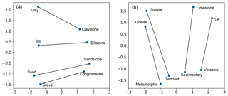
A different way of evaluating analogies is to plot the different pairs of words in a two-dimensional PCA projection. Fig. 5 shows different pairs of words which can be seen as group analogies. From the plot, any pair of related words can be expressed as an analogy. For example, from Fig. 5a, it is possible to generate the analogy “claystone is to clay as sandstone is to []? (sand)”, and the first model output is indeed “sand”.

As we showed in Fig. 2, the embeddings encode different relationships with different degrees of sophistication. In Fig. 5a it is possible to observe simple analogies, mostly syntactic as “claystone” contains the word “clay”. Figure 5b presents a more advanced relationship, where rock names are assigned to their corresponding rock type.

Figure 5 Two-dimensional PCA projection of selected words. Simple syntactic relationship between particle fraction sizes and rocks (a) and advanced semantic relationship between rocks and rock types (b).

6.4 Categorisation

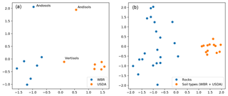
Similar to the analogies, the categorisation task can also present different degrees of complexity of the representations. In Fig. 6a, k-means clustering can distinguish the two expected clusters of concepts, WRB (FAO, 1988) and soil taxonomy (USDA, 2010) soil classification names. Andisols and Andosols are correctly assigned to their corresponding groups but are apart from the rest, probably due to their unique characteristics. Vertisols are correctly placed in between the two groups as both have a soil type with that name. A second level of aggregation can be observed in Fig. 6b. The k-means clustering correctly assigned the same soil groups from Fig. 6a into a general “soil types” group, different from “rocks”.

Figure 6 Two-dimensional PCA projection of selected categorisations. Clusters representing soil types from different soil classification systems (a) and a different aggregation level where the same soil types are grouped as a single cluster when compared with rocks (b).

6.5 Other embedding properties

Interpolation of embeddings is an interesting exercise that allows to further explore if the corpus is well represented by the vector space. Interpolation has been used to generate a gradient between faces (Yeh et al., 2016; Upchurch et al., 2017), assist drawing (Baxter and ichi Anjyo, 2006), and transform speech (Hsu et al., 2017). Interpolation between text embeddings is less common. Bowman et al. (2015) analysed the latent vector space of sentences and found that their model was able to generate coherent and diverse sentences when sampling between two embeddings. Duong et al. (2016) interpolated between embeddings from two vector spaces trained on corpora from different languages to create a single cross-lingual vector space. The vector space from our model also presents similar characteristics.

In order to generate the interpolated embeddings, we obtained linear combinations of two-word embeddings using the formula

$$\begin{array}{}\text{(4)}& {\mathit{v}}_{\mathrm{int}}=\mathit{\alpha }\times {\mathit{v}}_{\mathrm{a}}+(\mathrm{1}-\mathit{\alpha })\times {\mathit{v}}_{\mathrm{b}},\end{array}$$

where v_int is the interpolated embedding, and v_a and v_b are the embeddings of the two selected words. By varying the value of α in the range [0,1], we generated a gradient of embeddings. For each intermediate embedding obtained by interpolation, we calculated the cosine similarity (Eq. 3) against all of the words in the corpus and selected the closest one.

The results showed coherent concepts along the gradients (Fig. 7). The interpolation between “clay” and “boulder”, with fine and coarse size, respectively, yields a gradient of sizes as follows: clay < silt < sand < gravel < cobble < boulder. Another interpolation example, along with another type of relationship, is shown in Fig. 7b. The interpolation between the rocks “slate” and “migmatite” yields a gradient of rocks with different grades of metamorphism as follows: slate < phyllite < schist < gneiss < migmatite.

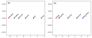
Figure 7 Interpolated embedding in a two-dimensional PCA projection showing a size gradient (a) with clay < silt < sand < gravel < cobble < boulder; and a gradient of the metamorphism grade (b) with slate < phyllite < schist < gneiss < migmatite. Red and blue dots represent selected words (“clay” and “boulder”, and “slate” and “migmatite”) and black dots represent the closest word (cosine similarity) to the interpolated embeddings.

6.6 Illustrative example

As a final, external evaluation of the embedding, we estimated average embeddings for each great group (soil taxonomy) of soils from 10 000 soil profiles descriptions. The convex-hulls at the soil order level (Fig. 8) show the same pattern reported by Hughes et al. (2017). Thanks to the unique characteristic of Histosols and the high diversity of this taxonomic group, they are easily differentiated in the two-dimensional projection, showing the highest variability. The rest of the soil orders overlap heavily as their differences are hard to simplify into a two-dimensional space. This overlap does not imply that the orders are not separable in a higher-dimensional space. Here we plot the first two principal components (PCs), which only account for 28.8 % of the total variance. This is probably the same reason for the overlap in the study by Hughes et al. (2017), as they account for 95 % of the total variance only after 36 PCs (i.e. their plot, also using the first 2 PCs, probably explains a low proportion of the total variance, similar to our example).

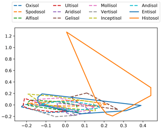
Figure 8 Convex-hulls of great group embeddings at the order level (soil taxonomy). Great group embeddings were obtained after averaging the embeddings of all the words in the descriptions of the profiles belonging to each great group. The convex-hulls were estimated from the two first principal components of the great group embeddings.

This example shows how, by using descriptions encoded as word embeddings, we were able to use the same methods as Hughes et al. (2017). In this case, if no soil variables (laboratory data) were available, word embeddings could be used instead. Ideally, we would expect to use word embeddings to complement numerical data and utilise valuable information included in the descriptive data. This is also possible with other approaches. Hughes et al. (2017) manually generated binary embeddings for the presence of ice and water. Another alternative to create embeddings is fuzzy logic. For example, McBratney and Odeh (1997) fuzzified categorical information from soil profiles such as depth, generating an encoding that represents the probability of belonging to different depth classes (e.g. a “fairly deep” soil could lay between the “shallow” and “deep” classes, with a membership of 0.5 to each class). The advantage of using word embeddings is that they are high-dimensional vectors that encode much more information applicable to many tasks, which would be difficult to replicate by manual encoding.

6.7 What do these embeddings actually represent?

It is worth discussing if word embeddings tell us anything about nature or if they really just tell us about the humanly constructed way that science is done and reported. A language model extracts information from the corpora to generate a representation in a high-dimensional space. This continuous vector space shows interesting features that relate words to each other, which were tested in multiple tasks designed to evaluate the syntactic regularities encoded in the embeddings. Considering the position that science is a model of nature (Gilbert, 1991) and assuming that the way we do and report science is a good representation of it, if the language model is a good representation of the corpora of publications, perhaps the derived syllogism – the language model is a good representation of nature – can be considered as true. Of course, the representation of a representation carries many impressions, but it is worth exploring its validity.

As shown by the linear combinations of embeddings (Fig. 7), some aspects related to “size” are captured by the embeddings and, even if size categories are a human construct, they describe a measurable natural property. A more complex case is the illustrative example, where the embeddings capture some aspects of nature which are also captured by the numerical representation of its properties (in this case soil properties such as clay content, pH, among others). Given the results of the intrinsic evaluation of this work and others referenced throughout this article, it is probably impossible to generate the “perfect embeddings”. Even if we were able to process all of the written information available, and ignore the limitations of any language model, the embeddings would still be limited by our capacity to understand non-linear relationships (Doherty and Balzer, 1988) and, in turn, to understand nature.

Whether word embedding can give new insights about geosciences is still to be tested. Studies in other fields have shown some potentially new information. For instance, Kartchner et al. (2017) generated embeddings from medical diagnosis data and, after performing a clustering, they found clear links between some diagnoses related to advanced chronic kidney disease. Some of the relations are already known and accepted by the medical community, whereas others are new and are just starting to be studied and reported.

6.8 Future work

In the future, we expect to evaluate the effect of using our embeddings in more downstream applications (extrinsic evaluation). It is expected that domain-specific embedding will necessarily improve the results of downstream tasks but this is not always the case. Schnabel et al. (2015) suggested that extrinsic evaluation should not be used as a proxy for a general notion of embedding quality, as different tasks favour different embeddings, but they are useful in characterising the relative strengths of different models. We also expect to expand the test suite with more diverse and complex tests, opening the process to the scientific community. Another interesting opportunity is the inclusion of word embeddings in numerical classification systems (Bidwell and Hole, 1964; Crommelin and De Gruijter, 1973; Sneath et al., 1973; Webster et al., 1977; Hughes et al., 2014) which try to remove subjectivity by classifying an entity (soil, rock, etc.) based on numerical attributes that describe its composition.

7 Conclusions

In this work we introduced the use of domain-specific word embeddings for geosciences (GeoVec), and specifically soil science, as a way to (a) reduce inconsistencies of descriptive data, and (b) open the alternative to include such data into numerical data analysis. Comparing the result with general domain embeddings, trained on corpus such as Wikipedia, the domain-specific embeddings performed better in common natural language processing tasks such as analogies, terms relatedness, and categorisation, improving the overall accuracy by 107.9 %.

We also presented a test suite, specifically designed for geosciences, to evaluate embedding intrinsic performance. This evaluation is necessary to test if syntactic or semantic relationships between words are captured by the embeddings. The test suite comprises tests for three tasks usually described in the literature (analogy, relatedness, and categorisation) with different levels of complexity. As creating a set of gold standard tests is not a trivial task, we consider this test suite a first approach. In the future, we expect to expand the test suite with more diverse and complex tests and to open the process to the scientific community to cover different subfields of geosciences.

We demonstrated that the high-dimensional space generated by the language model encodes different types of relationships, using examples of soil-related concepts. These relationships can be used in novel downstream applications usually reserved for numerical data. One of these potential applications is the inclusion of embeddings in numerical classification. We presented an example were we successfully emulated part of a taxonomic analysis of soil profiles which was originally applied to soil numerical data. By encoding soil descriptions as word embeddings we were able to utilise the same methods used in the original application and obtain similar results. Ideally, we would expect to use word embeddings when no numerical data are available or to complement numerical data to include valuable information included in the descriptive data.