Soil respiration across a variety of tree-covered urban green spaces in Helsinki, Finland

As an increasing share of the human population is being clustered in cities, urban areas have swiftly become the epicentres of anthropogenic carbon (C) emissions. Understanding different parts of the biogenic C cycle in urban ecosystems is needed in order to assess the potential to enhance their C stocks as a cost-efficient means to balance the C emissions and mitigate climate change. Here, we conducted a field measurement campaign over three consecutive growing seasons to examine soil respiration carbon dioxide (CO₂) fluxes and soil organic carbon (SOC) stocks at four measurement sites in Helsinki, representing different types of tree-covered urban green space commonly found in northern European cities. We expected to find variation in the main drivers of soil respiration – soil temperature, soil moisture, and SOC – as a result of the heterogeneity of urban landscape and that this variation would be reflected in the measured soil respiration rates. In the end, we could see fairly constant statistically significant differences between the sites in terms of soil temperature but only sporadic and seemingly momentary differences in soil moisture and soil respiration. There were also statistically significant differences in SOC stocks: the highest SOC stock was found in inactively managed deciduous urban forest and the lowest under managed streetside lawn with common linden trees. We studied the impacts of the urban heat island (UHI) effect and irrigation on heterotrophic soil respiration with process-based model simulations and found that the variation created by the UHI is relatively minor compared to the increase associated with active irrigation, especially during dry summers. We conclude that, within our study area, the observed variation in soil temperature alone was not enough to cause variation in soil respiration rates between the studied green space types, perhaps because the soil moisture conditions were uniform. Thus, irrigation could potentially be a key factor in altering the soil respiration dynamics in urban green space both within the urban area and in comparison to non-urban ecosystems.

1 Introduction

Urbanisation and climate change are two topical themes in current discussion on the human–nature relationship. Over 55 % of the global population lived in urban areas in 2018, and that percentage is likely to increase in the near future (Das, 2021). Urban areas are notable sources of atmospheric carbon dioxide (CO₂) (Pataki et al., 2006; Canadell et al., 2009; Velasco and Roth, 2010), and since the most recent trend of rapid increase in atmospheric CO₂ concentration is due to human activity (Arias et al., 2021), many cities are currently setting up climate programmes with the aim of carbon (C) neutrality in the coming years or decades (European Commission, 2022). Carbon neutrality can be achieved by reducing C emissions, compensating for them, or maintaining and increasing C sinks and stocks in urban vegetation and soil, the last of which is often deemed the most cost-efficient option (Faivre et al., 2017).

When considering the different C stocks in nature, soil organic carbon (SOC) stock is of special interest because of its vast quantity: estimates of global SOC stock range between 1500 and 3000 Pg C (Eswaran et al., 1993; Scharlemann et al., 2014) – a magnitude which clearly exceeds the estimated global organic C stocks in aboveground vegetation or in the atmosphere (Lal, 2004; Scharlemann et al., 2014). SOC stock is formed by C inputs from aboveground and belowground litter, root exudates, and possible organic amendments (Davidson and Janssens, 2006; Basile-Doelsch et al., 2020). Even though only 2.7 % of global terrestrial soils are urban (Lal and Stewart, 2018), by utilising judicious management practices, urban ecosystems have potential to sequester and store C in soil and vegetation on a local scale (Lal and Augustin, 2012; Foldal et al., 2022), which benefits the aforementioned C neutrality goals of cities and municipalities.

However, the current understanding of the biogenic C cycle in urban environments is mostly based on dynamics observed in more intensively studied non-urban ecosystems, such as forests and agricultural lands. Urban ecosystems differ from non-urban ecosystems in terms of light availability, temperature, precipitation and water cycle, pollution, restrictions in soil volume and crown space, and the level of human-induced disturbance (Sæbø et al., 2003; Kaye et al., 2006), all of which have an impact on the urban biogenic C cycle (Lal and Augustin, 2012). The urban heat island (UHI) effect, caused by anthropogenic heat sources and heat stored and re-radiated by built structures, elevates air temperature in urban areas compared to their non-urban surroundings (Oke, 1982; Rizwan et al., 2008). The UHI effect also creates temperature variation within the urban area because of varying building density and the heterogeneity of land cover and land use types that comprise the urban landscape (Yan et al., 2014; Edmondson et al., 2016; Lan and Zhan, 2017; Johnson et al., 2020). Some urban green spaces are irrigated for various reasons during the growing season (Ignatieva et al., 2020; Cheung et al., 2021; Pan et al., 2023), which makes their soil moisture conditions notably different to areas under natural precipitation.

Many urban green spaces are constructed, during which their soil and other growing media are established based on multiple parallel needs. The land use history of a specific urban green space can be diverse and the lifespan of its current state not necessarily so long. As a result, there is often no evident coupling between the aboveground vegetation and the belowground C in urban green spaces that is often found in more naturally developed ecosystems (e.g. Frouz et al., 2009; Pinno and Wilson, 2011; Dantas et al., 2020); observed SOC stock tends to represent the decisions made and actions taken while establishing the particular green space rather than reflect the current aboveground vegetation and its dynamics.

Soil respiration (R_S) is the CO₂ flux from soil surface to atmosphere that results from belowground plant and microbial respiration (Ryan and Law, 2005), and it is the second-largest terrestrial carbon flux (Bond-Lamberty and Thomson, 2010; Lei et al., 2021). It can be further classified into autotrophic (R_A) and heterotrophic (R_H) respiration, of which the former originates from plants and their roots and the latter from fungi, bacteria, and animals living in soil and litter (Burba, 2022). In practice, R_S is the key pathway through which C transfers from SOC stock to the atmospheric C stock as SOC is decomposed by microbial activity (Davidson and Janssens, 2006). Soil temperature and moisture are important controls for R_S (Bond-Lamberty and Thomson, 2010; Burba, 2022), and the SOC stock size itself also affects the decomposition rate (Davidson and Janssens, 2006).

Measurement-based estimates of SOC stocks in urban green space have been reported in previous literature and shown to vary across climatic conditions. In cold and temperate climates, the estimates for SOC stock in urban parks range between 9.7 and 35.5 kg C m⁻² depending on the aboveground vegetation type, management type, and park age (Pouyat et al., 2006; Dorendorf, 2014; Setälä et al., 2016; Lindén et al., 2020; Cambou et al., 2021). Areas with the most intensive management practices have been reported to have the highest SOC stocks, and these may be more than 2 times larger (per area) than in natural grasslands and agricultural lands (Pataki et al., 2006; Golubiewski, 2006). Two studies conducted in Helsinki (Finland) also observed high SOC stocks (19.5 kg C m⁻²) in park soils under the most intensive management class (Setälä et al., 2016; Lindén et al., 2020).

Previous studies measuring urban R_S are more scarce than estimates of SOC stock, but some indicators for specifically urban dynamics exist. Decina et al. (2016) measured R_S in urban soils in Boston (USA), finding up to 2.2 times higher R_S than that measured in the closest rural ecosystems. However, Weissert et al. (2016) observed that urban R_S in Tāmaki Makaurau / Auckland (New Zealand) was similar to non-urban forests and grasslands. Incorporating compost in urban soils, that is, increasing their SOC stock, was shown to increase R_S in Liverpool (UK) (Beesley, 2014). Goncharova et al. (2018) reported that in their measurements in Moscow (Russia), soil temperature was an important control for R_S in spring and autumn, whereas soil moisture was the main controlling factor during summer, when soil temperature was above 10 °C, which could imply that irrigation plays a significant role in summer. Wu et al. (2016) demonstrated how in Beijing (China) R_S was elevated at the boundary between urban green space and impervious surface as a result of a higher soil temperature. Conversely, R_S at urban forest edges in Boston has been shown to be reduced due to higher temperature and more probable aridity (Garvey et al., 2022), a phenomenon contrasting what has been observed in non-urban forests in Petersham (USA) (Smith et al., 2019).

The above, seemingly contradictory, examples demonstrate the need to (i) further characterise urban SOC stocks and R_S dynamics, (ii) consider urban ecosystems separately from non-urban ecosystems, and (iii) take into account the variation in environmental conditions within the urban area. In this study, we aimed to answer those needs by analysing R_S and its drivers in urban green space, focusing on the following research questions:

1. Can we observe differences in soil respiration rates measured in different types of tree-covered urban green space? If yes, are the differences only explained by consistent differences in soil moisture, soil temperature, or SOC stocks?

2. To what degree does the UHI affect the heterotrophic soil respiration rate during the growing season?

3. To what degree does irrigation affect the heterotrophic soil respiration rate during the growing season?

To answer these questions, we carried out a field measurement campaign in four different types of tree-covered urban green spaces in Helsinki over three consecutive growing seasons. Additionally, we used a process-based ecosystem model trained with the observations to specifically answer research questions 2 and 3 since controlled field experiments are difficult to perform, especially in the case of mature trees. Tested modelling tools are also needed for potential applications such as estimating C fluxes in urban nature in the future climate. We hypothesised that we would find different levels of soil moisture, soil temperature, and SOC across the green space types included in this study due to the heterogeneous urban environment and that these differences would also be reflected in differences in R_S rates. We also hypothesised that the UHI effect alone would have a notable effect on the R_S rate in urban ecosystems and that irrigation would allow for the R_S rate to remain at a higher level throughout the growing season than would be the case in non-irrigated environments under natural precipitation conditions.

2 Material and methods

2.1 Site description

This study was conducted in Helsinki, the capital of Finland, which in 2020 had a population of 656 920 (1 524 489 for the whole metropolitan area) and a population density of 3020 people per km² of land area (City of Helsinki, 2021). Average annual temperature and precipitation were 6.5 °C and 653 mm, respectively, during the reference period of 1991–2020 (Finnish Meteorological Institute, 2022). Almost 34 % of the city’s land area in 2021 (the total of which was 217 km² including inland waters) consisted of green space managed by the city (City of Helsinki, 2021). Our four measurement sites were located in the Kumpula and Hermanni districts in central Helsinki (Fig. 1). They encompassed a variety of green space types commonly found in northern European cities: an urban forest (Forest), a fruit garden (Orchard), a managed park (Park), and a road verge between a roadway and a sidewalk (Streetside).

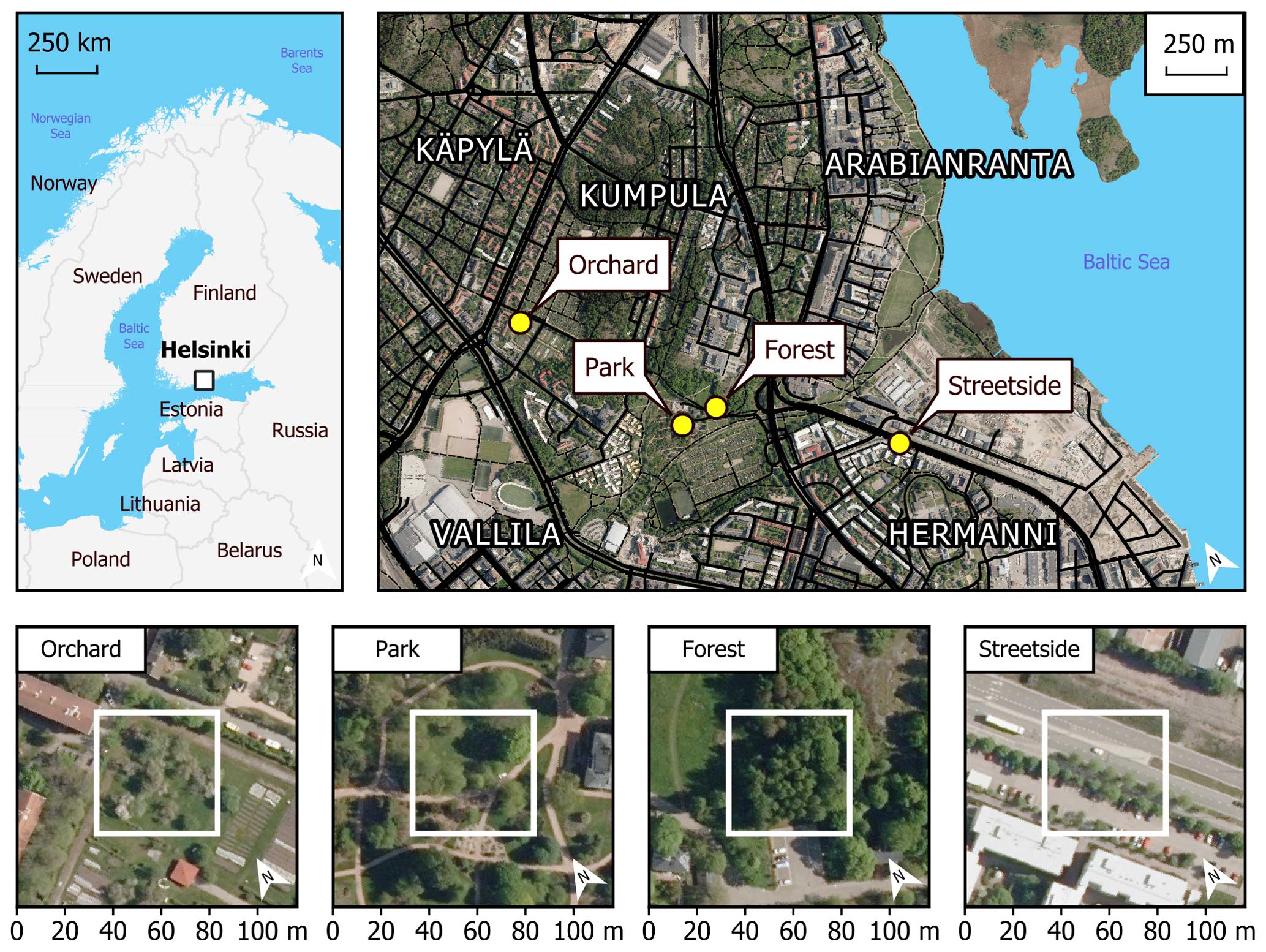
Figure 1 Four measurement sites (Orchard, Park, Forest, and Streetside) were located in the Kumpula and Hermanni districts in Helsinki (Finland). Site-specific panels (lower row) are scaled so the surroundings of each measurement site can be seen, while the white squares represent the more immediate locations where the manual measurements were conducted. Maps were built with the topographic database of the National Land Survey of Finland (2023), global administrative borders from GADM (2023), and orthophotos by the National Land Survey of Finland (2020).

The Forest site was situated at the edge of a small urban forest patch, with silver birch (Betula pendula Roth) being the dominant tree species. Other deciduous trees such as downy birch (Betula pubescens Ehrh.), Norway maple (Acer platanoides L.), and Scots elm (Ulmus glabra Huds.) formed the subcanopy. Understorey vegetation was sparse and consisted mainly of ground elder (Aegopodium podagraria L.). The Orchard site was comprised of apple trees (Malus domestica Borkh.) growing on a managed lawn. The lawn was mown manually a few times each summer and was not irrigated or fertilised. The Park site was located within the Kumpula Botanic Garden and consisted of four small-leaved linden trees (Tilia cordata Mill.) growing on a managed lawn. The lawn was mown daily by a mowing robot, fertilised once every few years, and irrigated during dry periods. However, the mowing robot could not access the section of the lawn on which the measurements were conducted; the lawn there was mown manually a few times each summer. The Streetside site was a row of common linden trees (Tilia × europaea L.) growing on a strip of managed lawn between a roadway and a sidewalk. The lawn was mown manually a few times each summer and was not irrigated or fertilised. The mean tree trunk diameter (diameter at breast height, DBH) at all sites was in a similar range (20–30 cm), but the standing tree volume was the largest at the Forest site because of the distinctively taller trees (22 m) compared to at the other sites (6.5–12.5 m) (Table A1). Some further descriptions of the sites can be found in Ahongshangbam et al. (2023).

2.2 Soil respiration measurements

In this study, manually measured soil respiration represents the sum of R_A and R_H with the respiration of ground and field layer vegetation (low enough to fit inside the measurement chamber) also included, and it is denoted with R_GF. Manual chamber measurements of R_GF were conducted weekly during the main growing season (May–September) in 2020–2022. The measurement setup consisted of a small cylindrical opaque steady-state chamber (V=0.007434 m³) equipped with an infrared CO₂ probe (GMP343; Vaisala Oyj, Vantaa, Finland), a relative humidity and air temperature sensor (HMP75; Vaisala Oyj), and a battery-powered fan to ensure air mixing within the chamber. Measurement data from the sensors were stored on site in a handheld data logger (MI70; Vaisala Oyj). On each measurement day, all sites were measured between 08:00 UTC+3 and 17:00 UTC+3. All measurement sites were not active in all study years; a detailed overview of the measurement schedule and some exceptions to the standard protocol are described in Fig. B1.

Eight chamber measurement points were systematically selected at each measurement site and the measurements were always performed at these fixed points. Overall, the aim of the selection was to capture the spatial variation within each measurement site by ensuring there is enough distance between the single measurement points and having some of them be located closer to trees than others, some closer to the edge of the green space than others, and so on. The measurement points were established along two parallel transects at Orchard and along two almost parallel transects at Forest and Park. At Orchard, the transects were situated 6 m apart from one another, and the measurement points on each transect were 6 m apart from each other. At Forest and Park, the transects were situated, on average, 4 m apart from one another and the measurement points on each transect were, on average, 3 m apart from each other. As the Streetside site was a less than a 2.5 m wide strip of lawn between a roadway and a sidewalk, there was not enough space for multiple parallel transects. Therefore, the measurement points were situated along a single stretch of 17 m in such a way that (i) there were 1–2 m in between the single measurement points and (ii) they covered the whole width of the lawn strip, with some points being closer to the roadway and some to the pavement.

A steel base frame for the chamber was installed at each point at two of the sites (Forest and Park), whereas mobile base frames were used at the other sites (Orchard and Streetside) because permanent installations would have prohibited regular activities (e.g. lawn mowing and recreational use) at the sites. The base frames were gently inserted 0.5–2 cm into the soil in order to avoid damaging the vegetation, while still allowing for an airtight seal. After insertion, the height of the mobile base frame was measured to determine the total chamber headspace volume needed to calculate the flux. The heights of the permanent base frames were monitored and re-measured at least a few times each year. The closure time of a single chamber measurement varied between 4 and 5 min, and the chamber was well ventilated between measurements. Data quality was monitored visually on site by observing the increasing trend of CO₂ concentration within the chamber, and the measurements were repeated if the quality was deemed insufficient.

2.3 Ancillary measurements

Soil temperature at each chamber measurement point was measured (at 10 cm depth) during the chamber measurement with a handheld soil thermometer (Pt100 and HH376; Omega Engineering Inc., Connecticut, USA). Soil moisture was measured (at 10, 20, 30, and 40 cm depths) with a soil profile probe (PR2; Delta-T Devices, Cambridge, UK) concurrently with the chamber measurements (see Fig. B1 for more details). Six fibreglass access tubes (ATS1; Delta-T Devices) were installed at each site. They were not co-located with the chamber measurement points but were scattered around the measurement site with the aim of capturing the spatial variation within the site. Three readings were obtained from each tube while horizontally rotating the profile probe 120° in between to ensure spatial representativeness to all directions (Delta-T Devices Ltd., 2016). Data were stored on site in a handheld data logger (HH2; Delta-T Devices). During the campaign years, a number of access tubes at Streetside broke down due to management and construction with heavy machinery. As a result, new tubes were installed to replace the broken ones. However, this led to some variation in the number of tubes measured each week.

Soil moisture readings were first averaged separately for each depth and over each access tube. The tubes at each site were then compared to each other, and anomalous single readings were discarded (a total of 4 – one at Forest and three at Park). If a tube constantly provided data that were notably different to the others, all readings from that tube were discarded (a total of two – both at Streetside).

2.4 Soil sampling, analysis, and stock calculation

Three types of soil samples were collected from all sites at some point during the campaign years. Particle size distribution, soil pH, and concentrations of various nutrients were analysed at a commercial lab (Eurofins Viljavuuspalvelu Oy, Mikkeli, Finland). By pooling together 16–18 individual soil core samples collected at 0–30 cm depth with a thin auger (d=2.3 cm), 1 L of soil was collected at Forest, Garden, and Streetside. At Orchard, four individual soil core samples were collected with a larger auger (d=5.0 cm). The particle size distribution was analysed according to Elonen (1971).

Samples for soil density were collected by inserting a steel cylinder (V=0.151 dm³ at Orchard and V=0.2 dm³ at the other sites) horizontally into an undisturbed soil profile at 10 cm depth. The fully inserted cylinder was gently detached with the sampled soil inside it to achieve volumetric accuracy. The samples were dried at 105 °C for 48 h and the dry weights were weighed. Soil density was then calculated by dividing the sample dry weight with the cylinder volume. Five individual samples were collected at Streetside, Park, and Forest and three samples at Orchard.

Six individual soil core samples were collected at 0–30 cm depth at each site with a soil auger (d=1.7 cm at Orchard and d=2.3 cm at the other sites) to analyse SOC and soil organic nitrogen (SON) content. The samples were sieved with a 2 mm mesh sieve and dried at 105 °C for 24 h, after which the dry weights of the smaller and larger grain size classes were weighed. The samples from Orchard were, however, sieved only after drying. Total soil SOC and SON contents were determined from the dried and milled samples of soil with a grain size smaller than 2 mm with an elemental CN analyser (LECO, Michigan, USA). The results were adjusted based on the site-specifically averaged proportion of soil with a grain size larger than 2 mm, assuming its SOC and SON content to be zero. Consequently, SOC and SON stocks (for 0–30 cm depth) were calculated utilising the averaged soil density at each site.

2.5 Flux data processing

CO₂ concentration measured with Vaisala GMP343 is dependent on air pressure, air temperature, relative humidity (RH), and oxygen (O₂) concentration (Vaisala, 2007). We used the automatic compensation procedures of the MI70 software to compensate for the effect of air temperature and RH by utilising real time air temperature data from GMP343's internal temperature sensor and RH data from an HMP75 sensor attached to the chamber measurement setup. We checked the prevailing air pressure at the Kumpula weather observation station (Finnish Meteorological Institute, 2023) operated by the Finnish Meteorological Institute (FMI) (60°12^′14.0^′′ N, 24°57^′38.9^′′ E; located 200–1000 m from the measurement sites) at the beginning of each measurement day and used that as an input for the automatic air pressure compensation for all measurements conducted during the day. As a constant for the O₂ concentration compensation for all measurements, 21.0 % was used.

The first 30 s of data were truncated from the beginning of each measurement in order to allow for the chamber headspace air to stabilise after closing the chamber. Then, the soil respiration CO₂ flux (R_GF) was calculated with Eq. (1):

$$\begin{array}{}\text{(1)}& {\mathrm{R}}_{\mathrm{GF}}={\left({\displaystyle \frac{\mathit{\delta }C\left(t\right)}{\mathit{\delta }t}}\right)}_{t=\mathrm{0}}\times {\displaystyle \frac{M\times P\times V}{R\times T\times A}},\end{array}$$

in which ${\left(\frac{\mathit{\delta }C\left(t\right)}{\mathit{\delta }t}\right)}_{t=\mathrm{0}}$ is the time derivative (CO₂ ppm s⁻¹) of a linear regression during a single chamber closure, M is the molecular mass of CO₂ (44.01 g mol⁻¹), P is the ambient air pressure during each measurement day (Pa), V is the total system (chamber and collar) volume (m³), R is the universal gas constant (8.31446 J mol⁻¹ K⁻¹), T is the mean temperature (K) inside the chamber during the closure, and A is the basal area (m²) of the chamber. The fits of all linear regressions were visually inspected, and the start and end points were adjusted if the fit quality was insufficient. If the adjustments did not lead to an acceptably linear fit or the eventual measurement duration after the adjustments would have been less than 2 min, the measurement was discarded.

2.6 Statistical analyses

To analyse for differences in R_GF, soil temperature, and soil moisture between the sites on a weekly level, a Kruskal–Wallis rank sum test (e.g. Hollander and Wolfe, 1973) was performed separately for each week's data (all years separately). When the resulting p value was statistically significant (p<0.05), a pairwise Wilcoxon rank sum test was used as a post hoc test to identify the site pairs with statistically significant (p<0.05) differences. The Benjamini–Hochberg method (Benjamini and Hochberg, 1995) was utilised to correct for multiple testing while performing the Wilcoxon rank sum tests. Non-parametric tests were used because of the non-normal distributions of the studied variables. The dataset used in the weekly analysis is depicted with green, blue, yellow, and grey in Fig. B1.

After the analyses on a weekly level, linear mixed-effects (LME) models were used to analyse for differences between the sites when all years and weeks were pooled together. For the purposes of this analysis, the data were filtered to include only (1) the R_GF measurements that had concurrent soil temperature and soil moisture data and (2) the days when all intended sites had been measured during the same day. This dataset included a total of 1473 chamber measurements and is depicted with green and grey in Fig. B1. R_GF, soil temperature, and soil moisture data were log-transformed before model building to enhance normality.

Separate LME models were built for R_GF, soil temperature, and soil moisture; all of them had site ID as a fixed effect and a week number and measurement point ID (access tube ID in the case of soil moisture data) as random effects (intercept) to account for the temporal (i.e. seasonal cycle; see Fig. C1a) and spatial (i.e. repeated measurements at the same measurement points) hierarchies in the field design, respectively. The month number was also tested as a random effect, but using the week number improved the model performance according to Akaike's information criterion (AIC). Including the year as a random effect was also tested, but it was left out of the final model structure as it did not improve the model performance according to AIC. All models were fitted with restricted maximum likelihood (REML). The normality of model residuals was inspected with quantile–quantile (Q–Q) plots, and model quality was ensured with conditional R². After building the models, estimated marginal means (EMMs) were computed for each site to allow for pairwise comparison.

Kruskal–Wallis and Wilcoxon rank sum tests were also used to test for differences between the measurement sites in terms of soil density, SOC and SON content, and SOC and SON stock, utilising the soil sample data. Additionally, we calculated the mean R_GF rate at each measurement site separately for each of the study years 2020–2022 and compared them to the site-specific soil characteristics (i.e. SOC and SON content and stock, soil density, P content, K content, pH, and soil particle size classes) by calculating Pearson correlation coefficients. All data analyses were conducted in R (R Core Team, 2023) v4.1.1–4.2.3 utilising the packages lme4 (Bates et al., 2015), multcompView (Graves et al., 2019), emmeans (Lenth et al., 2023), and MuMIn (Bartoń, 2023).

2.7 Ecosystem modelling

JSBACH (Jena Scheme for Biosphere–Atmosphere Coupling in Hamburg) (Reick et al., 2013) is a process-based land surface model and the land component in the Earth system model MPI-ESM of the Max Planck Institute for Meteorology (Giorgetta et al., 2013). Generally, it is used to study the coupled climate–carbon dynamics (Reick et al., 2021). Applications of JSBACH range from, for example, simulating the productivity of various ecosystems (see e.g. Wang et al., 2022; Trémeau et al., 2024) to studying the effects of land use change at various scales (see e.g. Tian et al., 2016; Arneth et al., 2017) and simulating specific phenomena and processes such as permafrost (Ekici et al., 2014), phenology (Bali and Collins, 2015), photosynthesis (Smith and Dukes, 2012), and natural disturbances (Lasslop et al., 2018).

In this study, we utilised JSBACH to model daily R_H at two of our measurement sites: Forest and Park. The model inputs included meteorological forcing data as well as parameters describing the vegetation and soil at the simulated sites. The meteorological forcing data were the same for both sites, but there were differences in the vegetation and soil parameters as outlined below.

The model was driven with hourly observation-based data of air temperature, precipitation, shortwave and longwave radiation, relative humidity, and wind speed. The dataset was compiled so that observations from the FMI Kumpula weather station (Finnish Meteorological Institute, 2023) were first gap-filled with observations from the closely co-located urban measurement station SMEAR III (Järvi et al., 2009), and any remaining gaps were then filled with hourly ERA5-Land data (Muñoz-Sabater et al., 2021). The gap-filled data were prepared for the period 2005–2022. To prepare long-term driver data needed for simulation spin-ups, ERA5-Land data were used from 1951 to 2004, and data prior to 1951 were randomly generated from the period 1951–1980.

In JSBACH, vegetation is represented by plant functional types (PFTs). The model was set up for simulating both sites using the PFT representing temperate broadleaf deciduous trees. Phenology is described in JSBACH with the Logistic Growth Phenology (LoGro-P) model (Böttcher et al., 2016), where the temporal development of leaf area index (LAI) of summer greens depends on temperature. The maximum LAI for each site was set based on Sentinel-2 data (Nevalainen et al., 2022; Nevalainen, 2022), and the seasonal LAI dynamics driven by temperature were simulated by the model. In addition, the phenology model parameters were adjusted separately for each site to match the bud burst in spring and the start of leaf shedding in autumn, both estimated from the Sentinel-2 data.

Soil texture classes for the sites were determined based on the soil particle size distribution analysed from the soil samples collected at the sites. Accordingly, the parameters describing the soil properties in JSBACH were then set to follow the recommendations by Hagemann and Stacke (2014), with the exception of volumetric field capacity and wilting point, which were site-specifically adjusted based on the manual soil moisture measurements at each site. The root depth of the forest and park sites were set to 0.65 and 0.45 m, respectively. We did not have measurement-based data on the tree root depth at the measurement sites. Therefore, root depth was determined utilising Crow (2005) as a starting point, from which the depths were then further adjusted (i) based on the estimated total soil layer thickness at our measurement sites and (ii) by comparing with the manual soil moisture measurements.

The description of the dynamics of litter and soil C in JSBACH is based on the Yasso07 model (Tuomi et al., 2009, 2011). The model has five C pools based on the chemical quality of the organic matter: (i) acid hydrolysable, (ii) water soluble, (iii) ethanol soluble, (iv) non-soluble and non-hydrolysable, and (v) humus. Pools i–iv are the so-called AWEN (acid, water, ethanol, non-soluble) pools. In addition, the model keeps track of the woody and non-woody organic material, i.e. litter, the difference between which is only the size of the litter elements. The AWEN litter pools are further divided into aboveground and belowground pools. This results in 18 C pools altogether. The C pools gain C from the litter flux and the root exudates from vegetation. Decomposition of the litter pools causes C to transfer both to other pools and to the atmosphere – that is, as R_H.

Each pool has a fixed loss rate determined at 0 °C with unlimited soil water. These loss rates are then dynamically modified based on temperature, water availability, and size of the woody litter elements. The decomposition rate of woody litter is slower than that of non-woody litter. It is assumed that the woody litter elements are larger and therefore decompose at a slower rate. The woody litter has a nominal size of 4 cm. The rates are reduced by multiplying with a size-dependent factor, which can be defined separately for each woody plant functional type. However, currently the same factor (0.53) is applied to all woody litter. In the case of non-woody litter, the factor is equal to 1. Yasso07 was originally calibrated with air temperature and precipitation and, in consequence, JSBACH simulates R_H using 30 d running averages of air temperature and precipitation from the meteorological forcing data, which co-vary with soil temperature and moisture. Soil temperature and moisture simulated by JSBACH are not used to calculate the R_H.

To study the impact of the UHI effect and irrigation on R_H, we conducted detailed simulations with modified meteorological forcing data for the study years 2020–2022. The effect of varying UHI strength was emulated by adding up to 2.0 °C to the observed air temperature in 0.5 °C increments. According to an air temperature measurement campaign around the Helsinki urban area in 2009–2010, 2.0 °C is a realistic premise for within-city air temperature variation as a result of UHI (Drebs, 2011). To emulate the effect of irrigation, an algorithm was created to increase the amount of precipitation in the forcing data based on the following criteria. Irrigation was applied from May to September, and the amount of water used for irrigation was estimated from summertime water consumption data obtained from the Kumpula Botanical Garden for 2019–2022. The need for irrigation was estimated based on both temperature and precipitation. We used 2-week averages; if either the average temperature over 2 weeks was above 19 °C or the average precipitation was below 1.4 mm d⁻¹ (∼20 mm over 2 weeks), we added 1.7 mm d⁻¹ irrigation as precipitation in the forcing data. When both conditions were met, irrigation was increased to 5.0 mm d⁻¹. This setup resulted in similar year-to-year variation in the emulated irrigation as what was seen in the water consumption data reported by the garden. In addition, a reference simulation was conducted using the unmodified forcing data, giving in total six simulations for each measurement site. All simulations included a common spin-up period of 8000 years for accumulating the soil C pools.

3 Results

3.1 Measured soil properties

Mean SOC contents (± standard deviation) at Forest, Orchard, Park, and Streetside were 3.4 % (±0.3), 2.5 % (±0.5), 3.3 % (±1.0), and 2.6 % (±0.6), respectively (Fig. 2a). The corresponding mean SON contents were 0.29 % (±0.02), 0.20 % (±0.03), 0.22 % (±0.05), and 0.13 % (±0.05) (Fig. 2b) resulting in C / N ratios of 11.9, 12.4, 15.0, and 20.1, respectively. Mean SOC stocks (in kg m⁻²) calculated for Forest, Orchard, Park, and Streetside were 10.9 (±1.0), 8.0 (±1.5), 8.6 (±2.6), and 7.4 (±1.8), respectively. The corresponding mean SON stocks (in kg m⁻²) were 0.92 (±0.07), 0.65 (±0.09), 0.57 (±0.12), and 0.37 (±0.15).

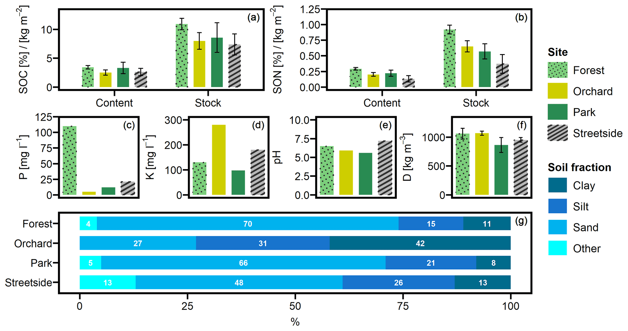
Figure 2 (a) Soil organic carbon (SOC) content and stock, (b) soil organic nitrogen (SON) content and stock, (c) phosphorus (P) content, (d) potassium (K) content, (e) pH, (f) soil density (D), and (g) particle size distribution were analysed from soil samples collected at the measurement sites (Forest, Orchard, Park, and Streetside). P, K, pH, and particle size distribution were analysed at a commercial lab. Grain size classes for sand, silt, and clay were 60–2000, 2–60, and <2 µm, respectively, and fraction Other refers to grain size larger than 2000 µm. Error bars denote standard deviation originating from multiple individual samples – if no error bars are shown, data originate from a pooled sample.

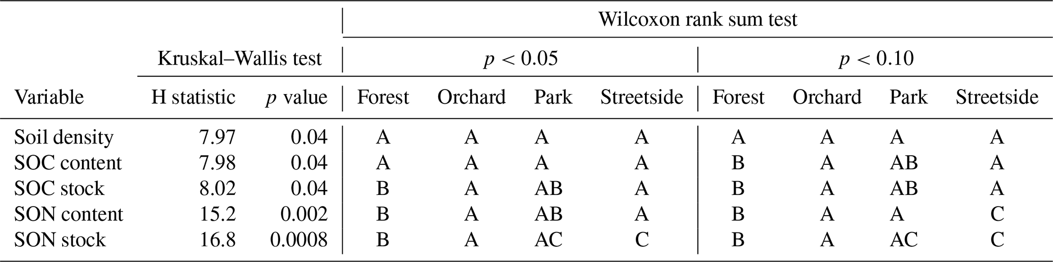
Overall, both SOC and SON stocks were the largest at Forest and the lowest at Streetside, with Orchard and Park situated in between and somewhat on the same level (Fig. 2a and b). The same pattern was also visible in the SOC and SON contents, although to a less pronounced degree. In terms of statistical significance (Table 1), SOC stock at Forest was significantly (p<0.05) larger than at Orchard and Streetside, but there was no significant difference between Forest and Park. SON stock was significantly (p<0.05) the largest at Forest and also significantly (p<0.05) larger at Orchard than at Streetside.

Soil phosphorus (P) content was distinctively higher at Forest compared to the other sites, and, similarly, potassium (K) content peaked at Orchard in comparison to the others (Fig. 2c and d). Differences in soil pH were less drastic, with Streetside having the highest and Park the lowest values (Fig. 2e). Soil density was the lowest at Park and the highest at Forest and Orchard, while Streetside was situated in between the two extremes although the differences between the extremes were small and statistically non-significant in pairwise comparison (Fig. 2f; Table 1). The particle size distribution at Orchard was notably different to the other sites as the share of clay reached 42 % and there were no particles with a grain size larger than 2000 µm (Fig. 2g). Consequently, when soil texture classes were determined for the sites according to the USDA classification (United States Department of Agriculture, 2017), Orchard was classified as clay, whereas the other sites were classified as sandy loam.

Table 1 Kruskal–Wallis test and Wilcoxon rank sum test results for differences in soil density, soil organic carbon (SOC) content and stock, and soil organic nitrogen (SON) content and stock between the measurement sites (Forest, Orchard, Park, and Streetside). First, the Kruskal–Wallis test was performed to detect whether there were statistically significant (p<0.05) differences, after which the Wilcoxon rank sum test was utilised for pairwise comparison between the sites. Two significance levels (p<0.05 and p<0.10) were utilised regarding the latter test, and statistically significant differences between the sites are denoted with letters A–C.

3.2 Measured R_GF, soil temperature, and soil moisture dynamics

Seasonal cycles were clearly visible in all of the three manually measured variables (Figs. 3, D1, and D2). R_GF and soil temperature increased until July, after which they started slowly decreasing towards autumn, and this pattern was rather similar in all study years. Soil moisture was generally at its highest in May and September and followed the precipitation events during the summer months. Its seasonal cycle had the most year-to-year variation as a result of varying precipitation regimes during the study years. For instance, there were a distinct local heatwave and drought in Helsinki during summer 2021 (see Ahongshangbam et al., 2023), which can also be seen in the decreasing trend in the measured soil moisture during June and July (Fig. 3). After the drought, a peak in R_GF was observed in the measurements of week 30.

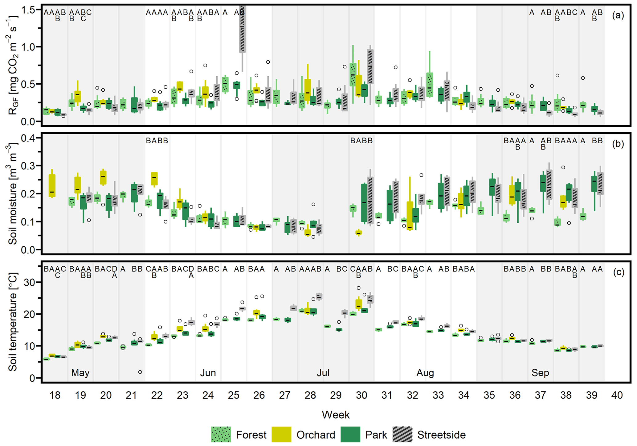
Figure 3 (a) Soil respiration (R_GF), (b) soil moisture (at 10 cm depth), and (c) soil temperature (at 10 cm depth) were measured weekly at four measurement sites (Forest, Orchard, Park, and Streetside) in 2021. Here, boxes are arranged chronologically by week number and the sites are always presented in the order that is shown in the legend. Background shading indicates the month. Empty circles are outliers. Letters A–D denote statistically significant (p<0.05) differences between the sites.

3.3 Differences in R_GF, soil temperature, and soil moisture between the sites

When considering the measurement data at a weekly level, the percentage of weeks (2020–2022 combined) that featured at least one statistically significant (p<0.05) difference between the sites in terms of either R_GF, soil temperature, or soil moisture was 33 %, 83 %, and 36 %, respectively. Thus, soil temperature is clearly the variable with the highest number of observed differences between the sites during our study period. Most commonly, Streetside differed from the others when data were available from there (2020–2021), but significantly higher momentary temperatures were also recorded in Orchard compared to the sites with higher tree cover density (Park and Forest). The differences occurred continuously throughout the study period, whereas the differences in R_GF and soil moisture were occurring less regularly, being perhaps slightly centred around the beginning and the end of the growing season, at least in 2021 and 2022 (Figs. 3 and D2). There also did not seem to be any clear causation of significant differences in soil temperature or moisture triggering significant differences in R_GF, as (i) the more infrequently occurring differences in R_GF and soil moisture did not necessarily co-occur and (ii) most of the weeks that featured significant differences in soil temperature did not feature differences in R_GF. Additionally, we did not find any statistically significant (p<0.05) correlations when comparing the site-specific yearly mean R_GF rates to the respective soil characteristics.

LME models (Table 2) were used to calculate the EMMs of the measured variables for each of the sites, utilising the whole dataset from 2020–2022. EMMs of R_GF (in mg CO₂ m⁻² s⁻¹) for Forest, Orchard, Park, and Streetside were 0.270, 0.273, 0.242, and 0.242, respectively, and there were no statistically significant (p<0.05) differences between the sites (Fig. 4a). EMMs of soil temperature (in °C) for Forest, Orchard, Park, and Streetside were 12.8, 13.7, 13.2, and 14.7, respectively (Fig. 4b). According to pairwise comparisons, Streetside was statistically significantly (p<0.05) the warmest measurement site, Orchard was significantly warmer than Forest, and there were no significant differences between Forest and Park or Park and Orchard. EMMs of soil moisture (in m³ m⁻³) for Forest, Orchard, Park, and Streetside were 0.137, 0.137, 0.150, and 0.164, respectively (Fig. 4c), and there were no statistically significant (p<0.05) differences between the sites. Regarding the random effects featured in the LME models, measurement point ID explained 24 %, 1 %, and 12 % of the leftover variance (i.e. after the fixed effects were considered) for the models of R_GF, soil temperature, and soil moisture, respectively, while week number correspondingly explained 30 %, 83 %, and 36 % (Table 2).

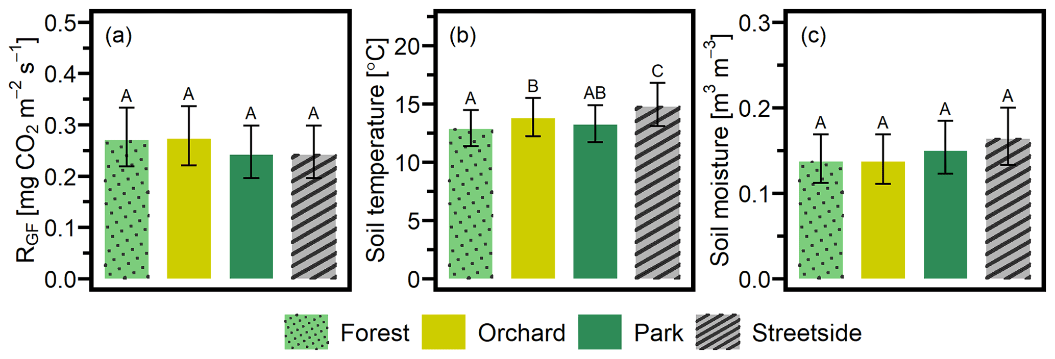
Figure 4 Three separate linear mixed-effects (LME) models were built to study the differences in (a) soil respiration (R_GF), (b) soil temperature (at 10 cm depth), and (c) soil moisture (at 10 cm depth) between the four measurement sites (Forest, Orchard, Park, and Streetside). Estimated marginal means (EMMs) were computed for each variable at each site, and the statistically significant (p<0.05) differences between the sites are reported with letters A–C. Error bars denote a 95 % confidence interval.

Table 2 Details of the three separate linear mixed-effects (LME) models that were built to assess the differences in soil respiration (R_GF), soil temperature (at 10 cm depth), and soil moisture (at 10 cm depth) between the four measurement sites (Forest, Orchard, Park, and Streetside).

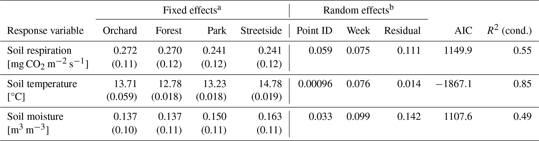
^a Fixed effects are reported as estimates (standard error). ^b Variance explained by the two random effects included in the models and the residual variance after the random effects were considered.

3.4 Model performance validation

To validate the model performance, we compared the temporal dynamics of the modelled R_H to the measured R_GF. Overall, the modelled R_H was considerably smaller (approximately 50 %) than observed R_GF but showed similar seasonal dynamics as R_GF in irrigated Park and non-irrigated Forest with a few exceptions (Fig. 5). First, observations included short peaks of high emissions after a rapid increase in soil moisture, especially in 2021, which were not predicted by the model. Second, the observed R_GF did not decrease like the non-irrigated (i.e. reference simulation) R_H in Forest in early 2022, but instead R_GF increased like R_H in the irrigated simulations before again following the non-irrigated R_H in the second half of the season (Fig. 5c). Lastly, the observed R_GF in Park did not increase like the predicted irrigated R_H, nor did it decrease like the non-irrigated R_H during July 2021 but stayed rather stable (Fig. 5e). Also, from mid-May to late August 2022, R_GF in Park was mostly quite stable unlike the modelled dynamics (Fig. 5f).

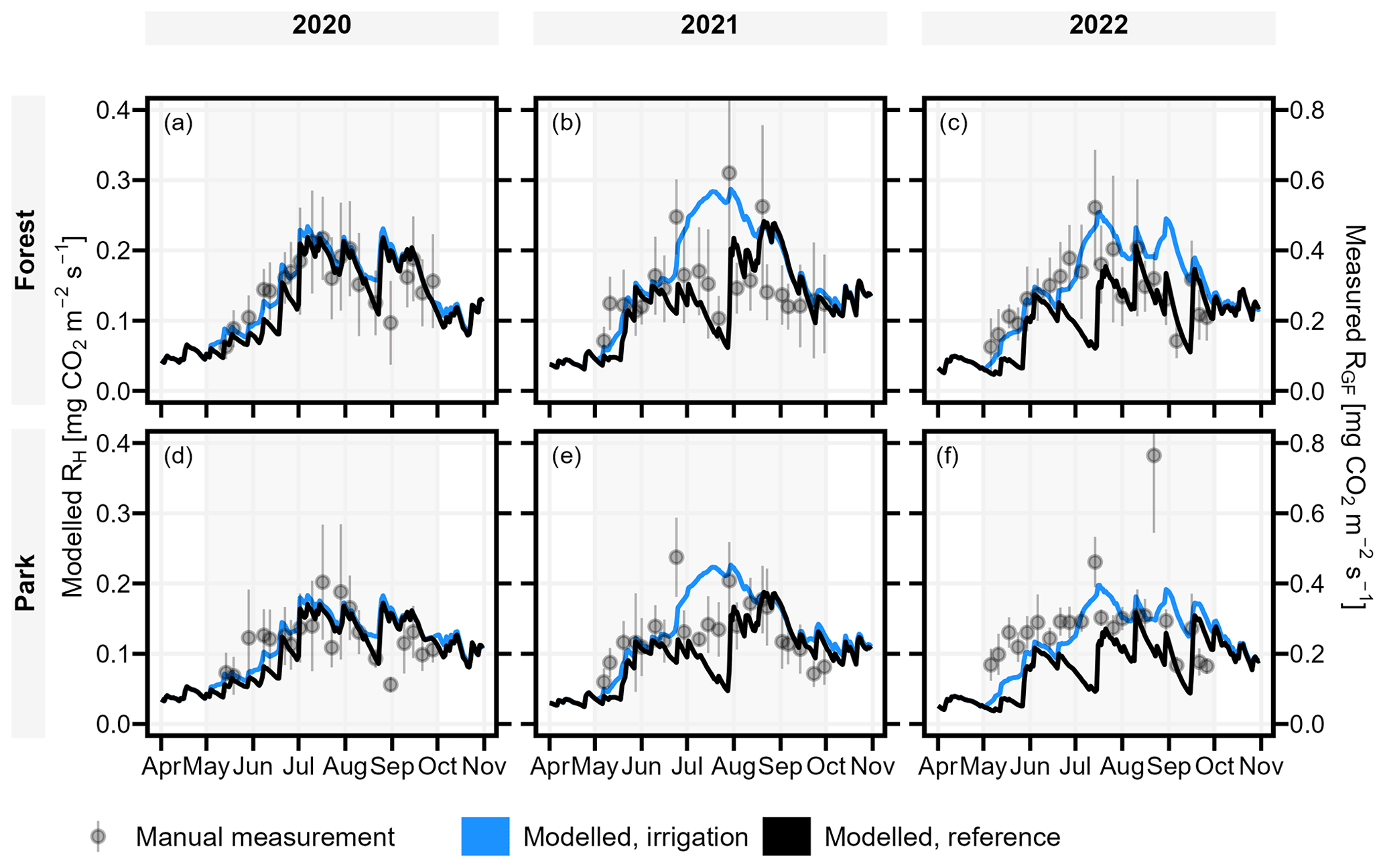
Figure 5 JSBACH modelled daily heterotrophic soil respiration (R_H; left axis) (both reference and irrigation simulation) showed similar temporal dynamics in comparison to the manually measured soil respiration (R_GF; right axis). Manual measurements are portrayed as mean ± standard deviation, and background shading indicates the study period (May–September).

3.5 Modelled impact of UHI and irrigation on R_H

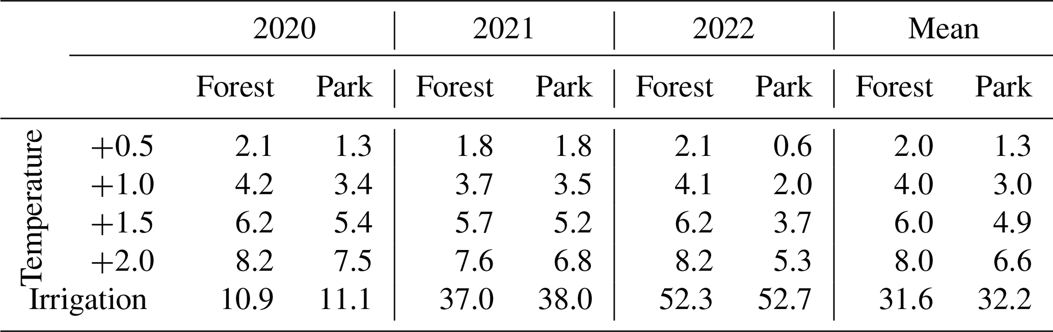
The modelled effect of elevated air temperature on R_H varied only slightly between the two measurement sites (Table 3, Fig. 6). When the daily mean momentary R_H fluxes were summed over the study period of May–September separately for each year (Table 3), an increase of 0.5 °C in air temperature increased R_H on average by 2.0 % and 1.3 % at Forest and Park, respectively. Based on the averaged results, an increase of 2 °C in air temperature within a city, as a result of the UHI, would result in a 6.6 %–8.0 % increase in local R_H CO₂ emissions depending on the green space type.

Simulated irrigation had a major effect in increasing R_H during the dry summers of 2021 and 2022, during which the relative increase in the cumulative R_H CO₂ emissions over the study period (May–September) was in the range of 37.0 %–38.0 % and 52.3 %–52.7 %, respectively (Table 3; Fig. 6). Again, the effect was considerably similar for both measurement sites. As the weather during the 2020 study period was more typical for Helsinki, the effect of irrigation was less pronounced (10.9 %–11.1 %), but even then the increase in R_H was more than what was seen with the elevated air temperatures.

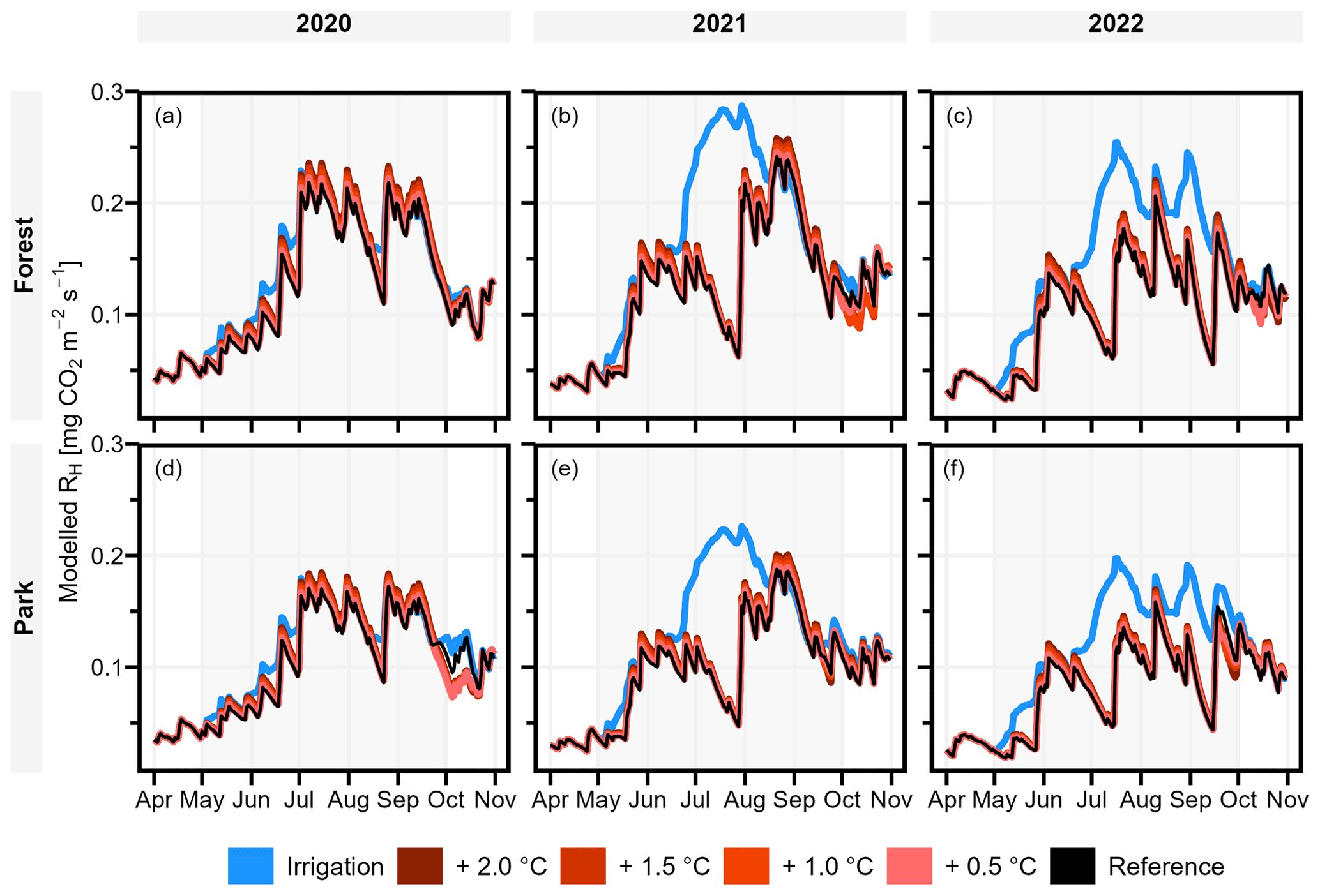
Figure 6 Daily heterotrophic soil respiration (R_H) at Forest and Park was modelled with JSBACH to study the effect of the urban heat island (UHI) and irrigation. During the study period of May–September (indicated with background shading), air temperature was increased by 0.5, 1.0, 1.5, and 2.0 °C, and an irrigation algorithm was used to simulate lawn irrigation during dry periods. A reference simulation was conducted separately for both measurement sites (Forest and Park), with the observed local weather conditions of each year.

Table 3 Daily heterotrophic soil respiration (R_H) at Forest and Park was modelled with JSBACH under varying environmental driver simulations. The daily carbon dioxide (CO₂) emissions were summed over the study period of May–September and compared to a reference run conducted with the observed local weather conditions of each year; positive values presented in the table imply an increase (in %) in R_H compared to the reference simulation. Results from the study years are shown both individually and as a mean of all study years.

4 Discussion

Quantifying the biogenic C stocks and C uptake potential in urban green spaces both now and in the future requires not only aboveground C stock estimates, but also an understanding of the soil and the C emissions arising from it. In this study, we collected data on R_GF and its main environmental drivers at four measurement sites representing different types of tree-covered urban green spaces expecting the drivers and, consequently, the resulting R_GF to differ among the sites. However, despite evident differences in management practices and standing tree volume, as well as in observed SOC and soil temperature, the observed R_GF was equal between the sites, except for momentary occasions.

Overall, the estimated marginal means (EMMs) of R_GF at the different green space types in May–September presented in the current study (Fig. 4) are of a similar order of magnitude (approximately 0.2–0.3 mg CO₂ m⁻² s⁻¹) to R_S measured in urban green spaces (forest, lawn, and landscaped) in Boston (Decina et al., 2016; Garvey et al., 2022) and under coniferous and deciduous trees in a botanical garden in Moscow (Goncharova et al., 2018). Wu et al. (2016) measured R_S specifically at the boundary between green space and impervious surface in Beijing; the mean momentary R_S values there were notably high, especially right at the impervious surface border, but in many cases decreased to a rather similar magnitude with our results when moving more than 1.5 m away from the border. The highest mean R_S rate they reported was 0.85 mg CO₂ m⁻² s⁻¹, which is something that was reached (and even surpassed) in our data during singular measurement weeks but not in seasonal means.

The currently measured urban R_GF rates were notably higher than some R_S rates measured in non-urban ecosystems in southern Finland, such as barley fields (on average 0.10–0.14 mg CO₂ m⁻² s⁻¹; Koizumi et al., 1999) or forestry-drained peatlands (R_H only, on average 0.08–0.10 mg CO₂ m⁻² s⁻¹; Minkkinen et al., 2007). In contrast, summertime forest floor R_S rates reported in southern (approximately 0.17–0.33 mg CO₂ m⁻² s⁻¹; Ryhti et al., 2022) and northern Finland (approximately 0.23–0.35 mg CO₂ m⁻² s⁻¹; Kulmala et al., 2019) were only slightly lower than our seasonal EMMs although our weekly R_GF rates during the peak summer months, June–August, tended to frequently exceed the range of the non-urban forest floor R_S. Similarly, summertime agricultural R_S rates reported by Heimsch et al. (2021) range, on average, between 0.23 and 0.35 mg CO₂ m⁻² s⁻¹. As our study lacks non-urban measurements to act as points of reference, we cannot reach such a clear conclusion of R_S in urban ecosystems being more than 2-fold in magnitude compared to their non-urban counterparts, as concluded by Decina et al. (2016), even though our results do support the premise of elevated R_S in urban areas.

In comparison to previous research, our measurements of SOC stocks in urban green space (on average 7.37–10.92 kg m⁻²) are similar to those measured in the top layers but on the lower end when compared to studies that measured SOC stocks down to 100 cm depth (Table 4). Differences in sampling depth make straightforward comparison difficult. Nevertheless, the stocks are still comparably or even notably higher than what has been measured in Finnish non-urban ecosystems – for example, in forest plots throughout Finland dominated by Scots pine (Pinus sylvestris L.) and Norway spruce (Picea abies (L.) H. Karst) (on average 5.49 and 8.32 kg m⁻², respectively, considering both organic layer and mineral soil; Lindroos et al., 2022) and in agricultural lands in Finland (on average 4.1–6.7 kg m⁻² for 0–15 cm depth; Heikkinen et al., 2013).

Riikonen et al. (2013)Setälä et al. (2016)Edmondson et al. (2014)Pouyat et al. (2006)Lindén et al. (2020)Edmondson et al. (2014)Pouyat et al. (2006)Pouyat et al. (2009)Lindén et al. (2020)Pouyat et al. (2006)Dorendorf (2014)Riikonen et al. (2017)Shchepeleva et al. (2017)Kaye et al. (2005)Pouyat et al. (2006)Bae and Ryu (2015)

Table 4 Soil organic carbon (SOC) stocks at various urban green space types reported in previous literature in comparison to the results of this study, arranged in descending order. The results of this study are reported as means of each measurement site. The bold font was utilised to highlight the results of this study.

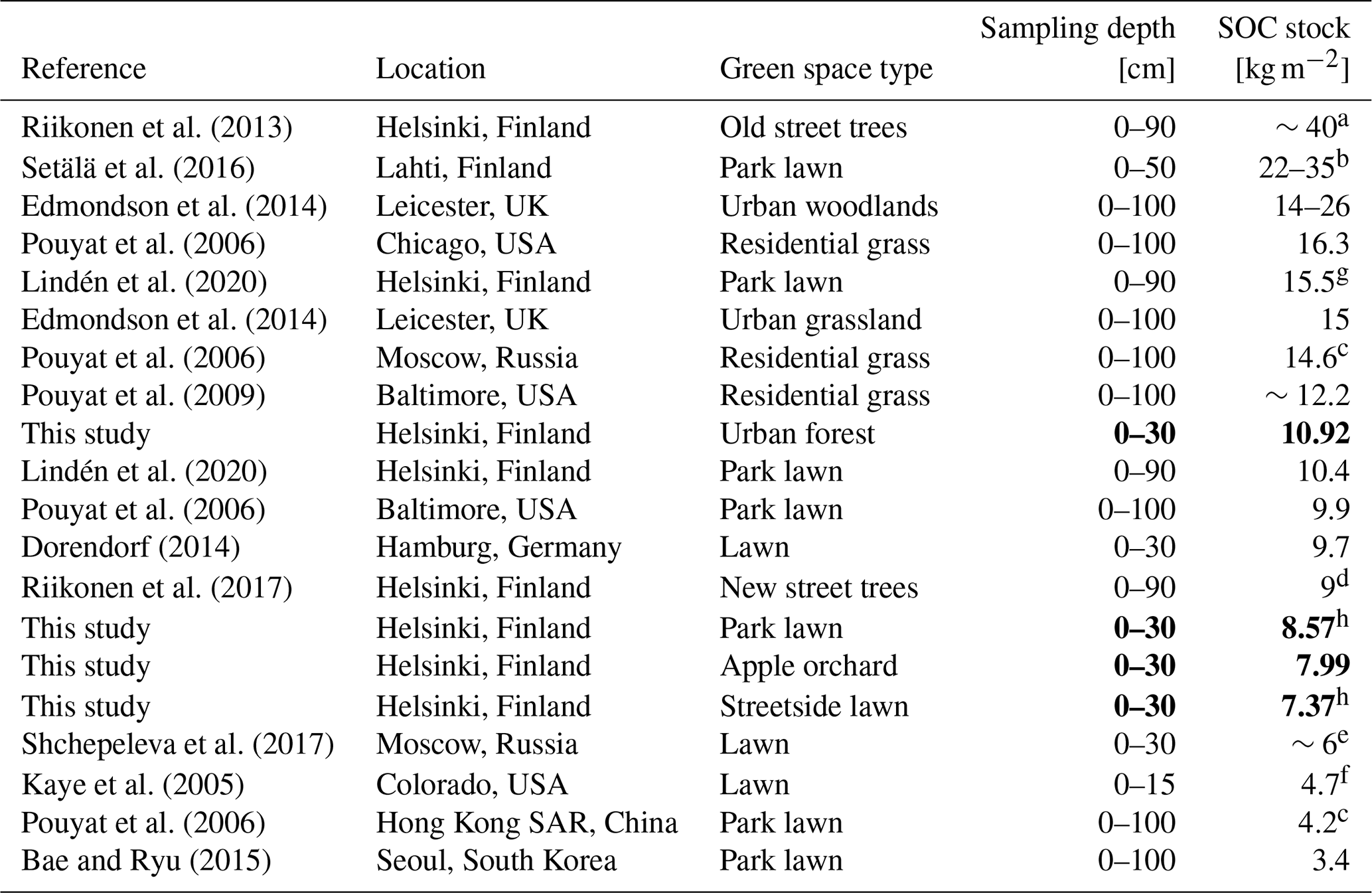
^a From restricted growing media. ^b Bulk density was not measured. ^c Calculated based on data from an earlier study. ^d Stone-based growing media. ^e Rather newly established lawn. ^f Irrigated and fertilised. ^g Under vegetation. ^h Under trees.

The highest SOC stock at our measurement sites was in a deciduous urban forest (Forest), where the litter C input to the soil is undoubtedly a lot higher than at the other sites that are under a more active management regime in terms of raking and removal of fallen branches, etc. This result would support the importance of non-intensively managed and infrequently disturbed urban forests, not only for their aboveground C stocks, but also especially for their SOC (see also e.g. Yesilonis and Pouyat, 2012; Lindén et al., 2020). Also, it needs to be noted that our measurement sites were of somewhat varying age (Table A1), which can have an impact on the observed SOC levels. In terms of temporal trends, urban SOC stock tends to first decrease as a result of construction and possible land use change, but can subsequently increase to a level surpassing that of non-urban areas (Pataki et al., 2006). Havu et al. (2022) inspected this in their modelling study; after constructing a new streetside green space, the annual R_S C emissions were high enough to supersede the amount of C sequestered annually by the newly planted street trees for the first 12–14 years after plantation. Our measurement sites mainly represent urban green spaces at such a life cycle stage in which the possible differences in SOC stock arising from the initial construction may have already levelled out, but the long-term development possibly still remains largely unseen.

Our initial hypothesis was that the overall heterogeneity typical of urban environments would be likely to establish varying levels of soil temperature and soil moisture at the four measurement sites – even though all of them were located within 2 km of each other. Indeed, soil temperature at Streetside was the highest of all measurement sites, which can most likely be explained by its surroundings: it was the site surrounded by the most extensive sealed surface cover and highest building density (see Fig. 1 and also Ahongshangbam et al., 2023) that were both likely to contribute to a more pronounced local UHI and consequently an elevated soil temperature. The soil temperature at Orchard was also significantly higher than at Forest, which could be explained by differences in their vegetation characteristics: at Orchard, the sparse apple trees grew on a lawn, whereas at Forest the measurement points were situated under a more closed canopy formed by distinctively taller trees, thus being effectively surrounded and shaded by the forest itself in all cardinal directions except for a small sector (i.e. forest edge) southwest. Therefore, Orchard was likely to receive more direct sunlight as a result of less shading from its surroundings, and more of that sunlight would have been reaching the ground level to warm up the soil due to lower tree cover density than what was the case at Forest.

Despite the observed significant differences in soil temperature, soil moisture levels were significantly different at the measurement sites only during some individual weeks, and there was no clear pattern of some sites being significantly different from others when analysing the dataset as a whole. Uniform soil moisture conditions could possibly be one of the prominent reasons for the fact that no significant differences were observed in R_GF either; according to Goncharova et al. (2018), soil moisture is the main factor controlling urban R_S during summer, when soil temperature has exceeded 10 °C. Another reason for the observed uniformity could be that SOC stocks at the sites were significantly different and the pattern was approximately the opposite of what was observed with soil temperature: the warmest site had the lowest SOC stock and vice versa. Since R_S is partly the result of decomposing SOC stock, a lower SOC stock to begin with could possibly permit the increase in R_S even with the observed elevated soil temperature. Although, drawing a rigid conclusion on such compensatory effects would warrant a more specifically tailored measurement setup than what this present study has to offer. Furthermore, there are also more controlling factors for R_S than the ones considered in this study: differences in the soil microbial community (Liu et al., 2018) or the level of dissolved organic carbon (DOC) (van Hees et al., 2005) between the measurement sites, for example, can also have influenced the results.

In general, the results of our LME analysis were in line with the findings of the week-level analysis. On a weekly level, soil temperature was the variable with the most frequently occurring statistically significant (p<0.05) differences between the measurement sites, and it was also the only variable with statistically significant differences between the sites in the LME analysis. The amount of variance explained by the random effects included in the LME models (Table 2) indicates that there was some systematic spatial variation in R_GF between the individual measurement points at each site, whereas there was hardly any variation in soil temperature. Previous research has also demonstrated R_S to commonly have notable spatial variation even at small scales (see e.g. Soe and Buchmann, 2005; Martin and Bolstad, 2009). Week number was especially good in explaining the temporal variation in soil temperature, which is likely due to it having the most pronounced seasonal cycle.

We expected a more pronounced effect of the UHI on R_H than found; comparing increases in R_H associated with either a minor increase in air temperature or active irrigation revealed the latter to be much more significant to the magnitude of the combined R_H CO₂ emissions of the growing season. On average, increasing air temperature by 2 °C increased R_H by less than 10 % compared to the reference run, whereas the increase produced by irrigation was 30 % higher – although in 2020, when the weather during the growing season was more typical for Helsinki than in the other (i.e. dryer) study years, the increase caused by irrigation was only slightly over 10 %. The small impact of temperature on R_H is supported by the small variation in measured R_GF between the measurement sites despite the significant temperature differences. At the same time, it must be noted that irrigation during drought will not only increase the C emissions by stimulating R_S, but also improve and sustain the livelihood of the vegetation and thus allow for more continuous and even increased C sequestration that can result in a net negative impact in the overall C balance of the ecosystem (see e.g. Wu et al., 2008; Olsson et al., 2014; Trémeau et al., 2024). Furthermore, irrigation has been shown to also lower soil temperature (Cheung et al., 2022a, b), which hinders R_S. Because of the multitude of intertwined factors determining the ultimate impact of irrigation on the C balance of an urban ecosystem, a properly controlled empirical experiment is still needed to reach credible conclusions. To add to the comparably short temporal viewpoint of this study, addressing the long-term effects of irrigation on SOC warrants further examination.

It is tricky to compare modelled R_H with the observations, which in this study also included the release of CO₂ during plant metabolic processes, that is, the R_A of tree roots, lawn, and other ground and field layer vegetation. Accurate observations of strictly R_H would enable a direct comparison, but such data are difficult to collect due to the interlinked nature of the different soil processes. For example, widely used root exclusion techniques, such as trenching, suffer from increased root litter, alterations in soil moisture, and changes in the activity and composition of microbial communities (Hanson et al., 2000; Ryhti et al., 2022). Also, the removal of belowground parts of ground vegetation, such as lawn, would affect the temperature and moisture of topsoil and thus also the heterotrophic activity. Consequently, utilising process-based models is a cost-efficient method of partitioning the R_S components.

The share of R_A in total soil respiration naturally depends on the amount of vegetation and on soil properties, such as fertility or the quality and quantity of soil organic matter (Mäki et al., 2022). Hanson et al. (2000) estimated that, on average, root respiration annually contributes 49 % of total R_S for sites with forest vegetation based on 37 published field-based studies. However, the share might change during the summer as the seasonal dynamics of root respiration in trees are influenced by environmental factors and phenological variations (Hopkins et al., 2013; Pumpanen et al., 2015). In this study, the simulated R_H was roughly 50 % of the observed R_GF, with no clear seasonal discrepancies. However, momentary changes in one might be hidden by opposite changes in the other.

As expected, the temporal patterns of the observations followed the irrigated simulation in the Park and the non-irrigated simulation in the Forest, with only a few exceptions. First, the observed R_GF in Park did not increase like the irrigated simulation in the year 2021. This difference is likely attributed to the actual irrigation scheme at that time, as the garden managers avoided watering the scientific instruments within our measurement site, resulting in somewhat less irrigation in comparison to most of the lawns within the park. Second, during the rainless period in early 2022, observed respiration in Forest did not decrease as predicted by the simulation, whereas the simulation accurately captured the subsequent reduction later in the season. This probably arises from increased autotrophic activity in the early season, as it is well known that roots are less sensitive to a decrease in topsoil moisture compared to heterotrophic activity (Ryhti et al., 2022) and that they can also acquire water from deeper soil layers. Therefore, we presume that most of the observed decreases in R_S during summer periods resulted from drought-restricted heterotrophic activity.

The Birch effect following a rain event in forest ecosystems is a widely recognised phenomenon (Birch, 1958; Jarvis et al., 2007). We can assume that some of the observed CO₂ peaks after a rapid increase in soil moisture probably arose from autotrophic activities, but the majority of them are most likely related to the fast breakdown of easily decomposable carbon substrates that have accumulated during the dry period. In an experimental field study, Unger et al. (2010) gained support for their hypothesis that rapid mineralisation of either dead microbial biomass or osmoregulatory substances released by soil microorganisms in response to hypo-osmotic stress is what is behind the phenomenon. However, the Yasso07 soil carbon model (Tuomi et al., 2009, 2011) included in JSBACH does not include such processes even though there are indications that sequential dry periods followed by heavy rains favour the accumulation of SOC compared with management schemes that maintain the soil moisture close to field capacity (Kpemoua et al., 2023). In the face of changing precipitation regimes and irrigation recommendations, understanding the long-standing impacts of the Birch effect and irrigation on the longevity of urban SOC in boreal regions requires further controlled experiments.

We aimed to carefully accommodate our modelling setup to the environmental conditions at the measurement sites to reduce uncertainty in the modelling results but, naturally, there are some possible sources of error stemming from the process. Most of the site-specific parameter values were altered based on observations of e.g. particle size distribution, soil moisture and LAI, while soil and root depth were estimated based on literature data and the soil depth in the area. Both approaches introduce potential sources of error, as observations can have their respective inaccuracies and drawing solely from literature lacks local verification. As an example, errors in the estimated soil and root depths could potentially change the drought response of the sites. Secondly, since the vegetation phenology at the sites was estimated based on LAI observations, errors in the observations would then in turn be reflected in the accuracy of the modelled phenology. We also assumed that the soil C pools at the simulated sites were in a steady state, which is not necessarily the case in the urban setting. Consequently, such uncertainties should be kept in mind while interpreting the modelling results.

Our study presents a valuable and temporally extensive dataset of chamber measurements of soil respiration and measurements of SOC stocks in urban green spaces, both topics that are still globally lacking measurement-based data. We acknowledge that a study setup with wider spatial coverage would have been useful in giving more grounds for conclusions regarding the specific characteristics of different tree-covered urban green space types. It would have been optimal to have more replicates of each type and to have them situated over a broader spatial scale within Helsinki, perhaps utilising land use or land cover data for a more nuanced site stratification approach. However, conducting measurements with such a spatially extensive setup would require much more resources and also hinder the frequency with which single sites could be visited compared to the temporal coverage that was achieved with the present setup.

It is hard to explicitly account for the singular effects of multiple important and co-affecting environmental variables in a field measurement setup like ours, in which the main idea is to measure the studied phenomena of interest (R_S) in the naturally varying environmental conditions rather than conducting measurements in a strictly controlled study setup. For example, our soil sampling design did not allow us to effectively delve into the specific effects individual soil characteristics (e.g. levels of various nutrients or the particle size distribution) could have had on R_S; collecting separate soil samples from each chamber measurement point would possibly have been a more effective approach to that. However, as the focus of this study was to examine the effects of soil temperature, soil moisture, and SOC, a different sampling design was eventually selected. Investigating the roles of both the soil per se and the soil microbial community on urban R_S would likely prove to be an interesting direction for future research.

5 Conclusions

As cities are becoming increasingly interested in utilising urban vegetation and soil to sequester and store carbon, measurement data are needed to properly understand the biogenic carbon cycle in urban ecosystems. We carried out an extensive field measurement campaign on soil respiration across a variety of tree-covered urban green spaces in Helsinki to investigate whether the varying urban structure would create variation in the key drivers of soil respiration and, consequently, affect the soil respiration rates. The management practices and standing tree volume between the sites were clearly different and the soils had statistically significant differences in soil temperature as well as soil organic carbon and nitrogen stocks, but the only differences in soil respiration we could distinguish seemed momentary and sporadic. Process-based model simulations showed that the increase in heterotrophic soil respiration over the growing season caused by elevating air temperature by 2 °C to simulate the urban heat island effect was lower than 10 %, whereas irrigation of urban green spaces created a stronger increase, averaging more than 30 %, and could reach over 50 % during a drier year. The observed consistency of modelled and measured data encourages the use of process-based models in simulating the urban biogenic carbon cycle.

Overall, our findings challenged some of our initial hypotheses and would encourage further studies on the topic, for example, utilising a measurement site setup with a broader spatial span, more site type replicates, and a more intricate take on soil characteristics including the soil microbial community. Based on our results, different soil temperature conditions are likely not the sole explanation for the previously discussed differences in the magnitude of soil respiration between urban and non-urban ecosystems – we cautiously emphasise the role of irrigation and soil moisture and hope to motivate further studies on the topic. We would also tend to agree with Decina et al. (2016) on the roles of possible organic amendments and the soil itself (especially soil organic carbon) in generating the differences in soil respiration between urban and non-urban ecosystems. Similarly, soil characteristics are likely an important factor in establishing variation in soil respiration within a city, but disentangling their specific effects from those of soil temperature and moisture was not in the scope of this study.

Appendix A: Measurement site details

Table A1 Vegetation and management characteristics at the measurement sites: main tree species; mean height (m) of the main tree species; mean diameter at breast height (DBH) (cm) of the main tree species; approximate age of the main tree species, i.e. years since plantation; ground vegetation type; and the presence of irrigation, fertilisation, and mowing.

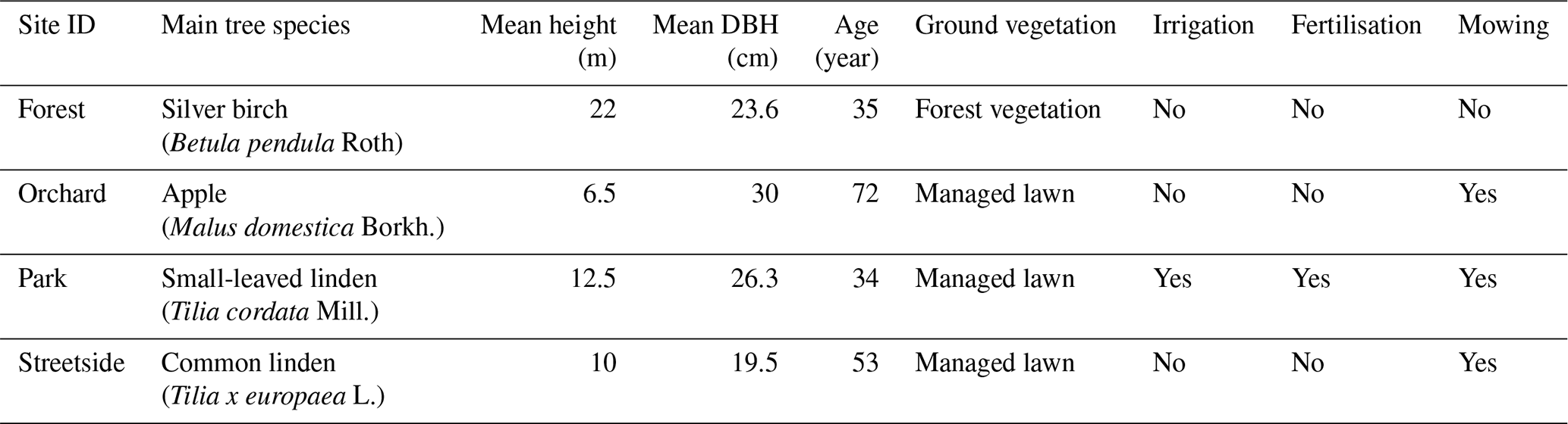
Table A2 Measurement site locations and soil characteristics. Values determined from multiple individual samples are given as mean (standard deviation), whereas other values represent a pooled sample. P, K, pH, and particle size distribution were analysed at a commercial lab.

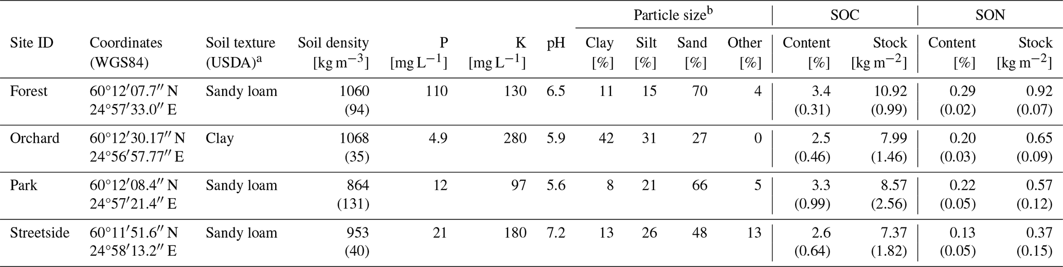
^a Soil texture class according to the USDA classification (United States Department of Agriculture, 2017). ^b Grain size classes for sand, silt, and clay were 60–2000, 2–60, and <2 µm, respectively, and fraction Other refers to grain size larger than 2000 µm.

Appendix B: Measurement dataset details

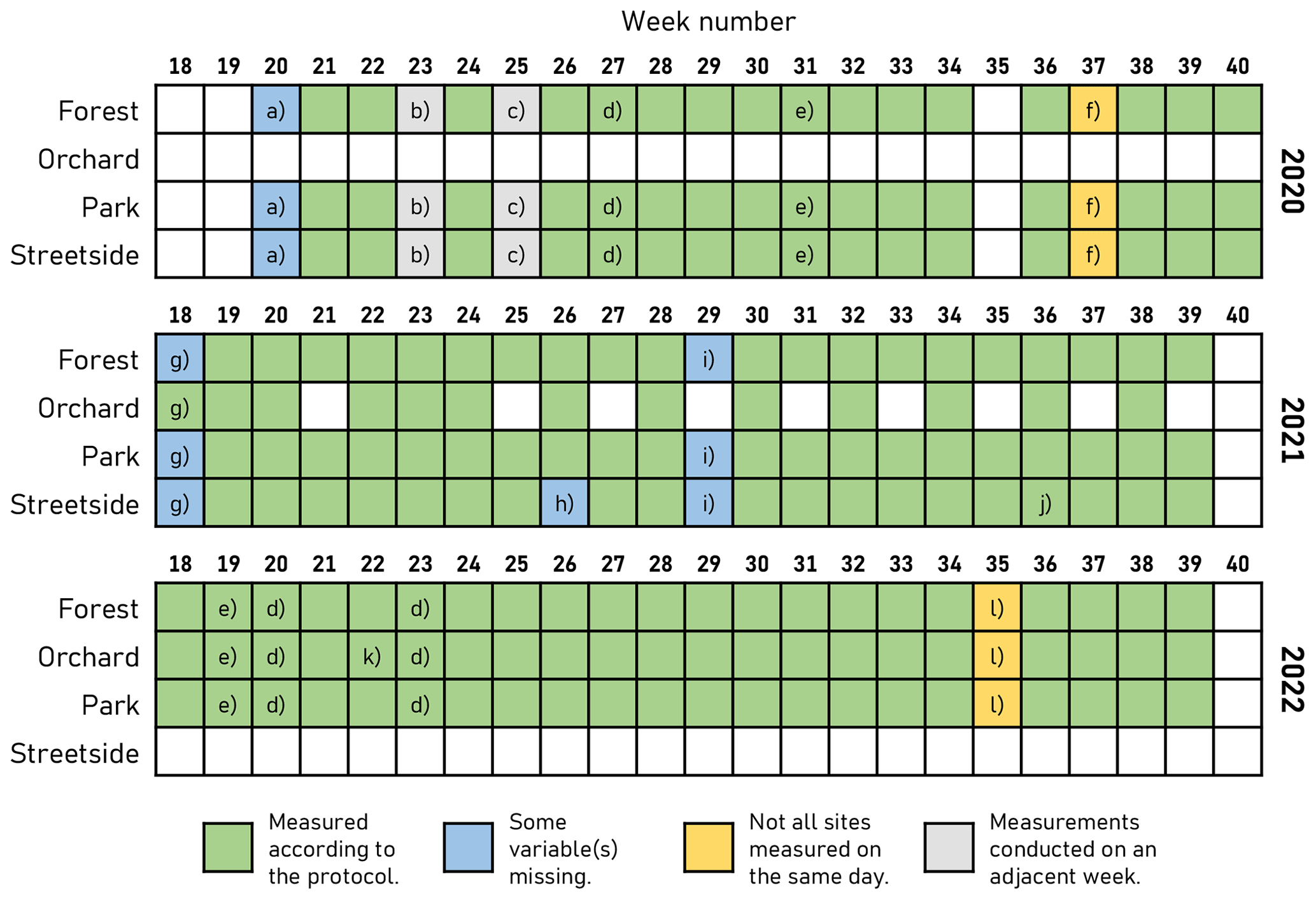
Figure B1 Overview of the schedule for manual soil respiration measurements and the concurrent soil temperature and soil moisture measurements. In case a, soil temperature and soil moisture were not measured. In case b, measurements were conducted on Monday of week 24, whereas measurements of week 24 were conducted on Friday. In case c, measurements were conducted on Monday of week 26, whereas measurements of week 26 were conducted on Friday. In case d, all measurements were conducted in the afternoon. In case e, all measurements were conducted in the afternoon, after some rain in the morning. Case f denotes that Park and Streetside were measured on Wednesday, whereas Forest was measured on Friday. In case g, soil moisture was measured only at Orchard. In case h, soil temperature was not measured at Street. In case i, soil moisture was not measured. In case j, soil temperature was missing from three measurement plots at Street (S6–S8). In case k, at Orchard, only two flux measurement plots (and their respective soil temperatures) were measured. Still, all soil moisture measurements were conducted. Finally, in case l, Forest and Park were measured on Tuesday, whereas Orchard was measured on Wednesday.

Appendix C: R_GF dataset for LME model building

Figure C1 All soil respiration (R_GF) measurements that were used in building the linear mixed-effects (LME) models. (a) All measurements from 2020–2022, grouped by site and arranged chronologically by week number. Sites are always presented in the same order that is shown in the legend. Outliers are marked with empty circles. (b–e) All measurements from each site pooled together separately for each year. Week number was added as a random effect in the models to account for the temporal hierarchy in the data, but the year was not included since there were no apparent differences between the three study years. Outliers are not portrayed in panels (b)–(e) to enhance clarity.

Appendix D: Weekly measurements of 2020 and 2022

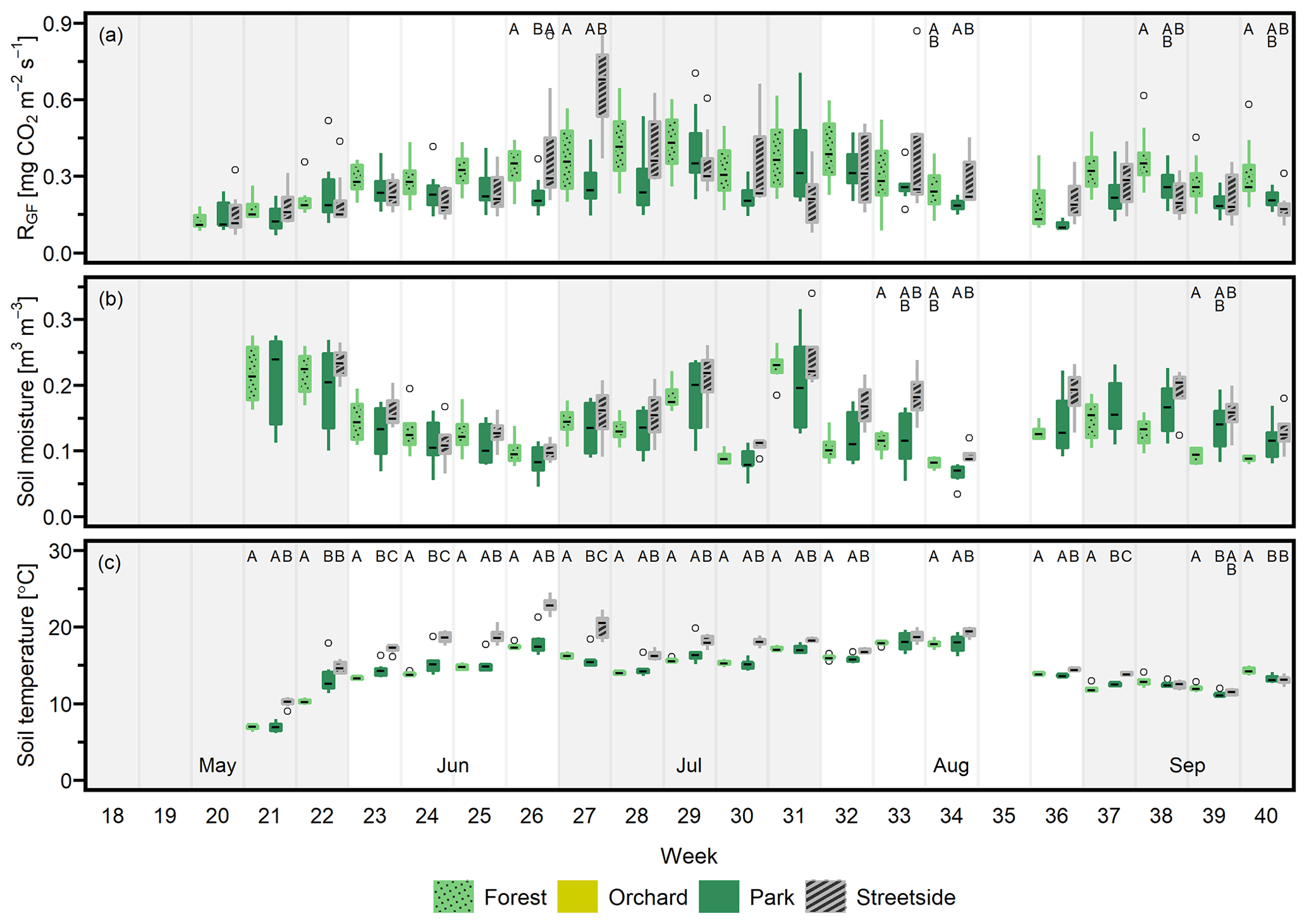
Figure D1 (a) Soil respiration (R_GF), (b) soil moisture (at 10 cm depth), and (c) soil temperature (at 10 cm depth) were measured weekly at three measurement sites (Forest, Park, and Streetside) in 2020. Here, boxes are arranged chronologically by week number and the sites are always presented in the order that is shown in the legend. Background shading indicates the month. Empty circles are outliers. Letters A–C denote statistically significant (p<0.05) differences between the sites. Note that Orchard was not measured in 2020.

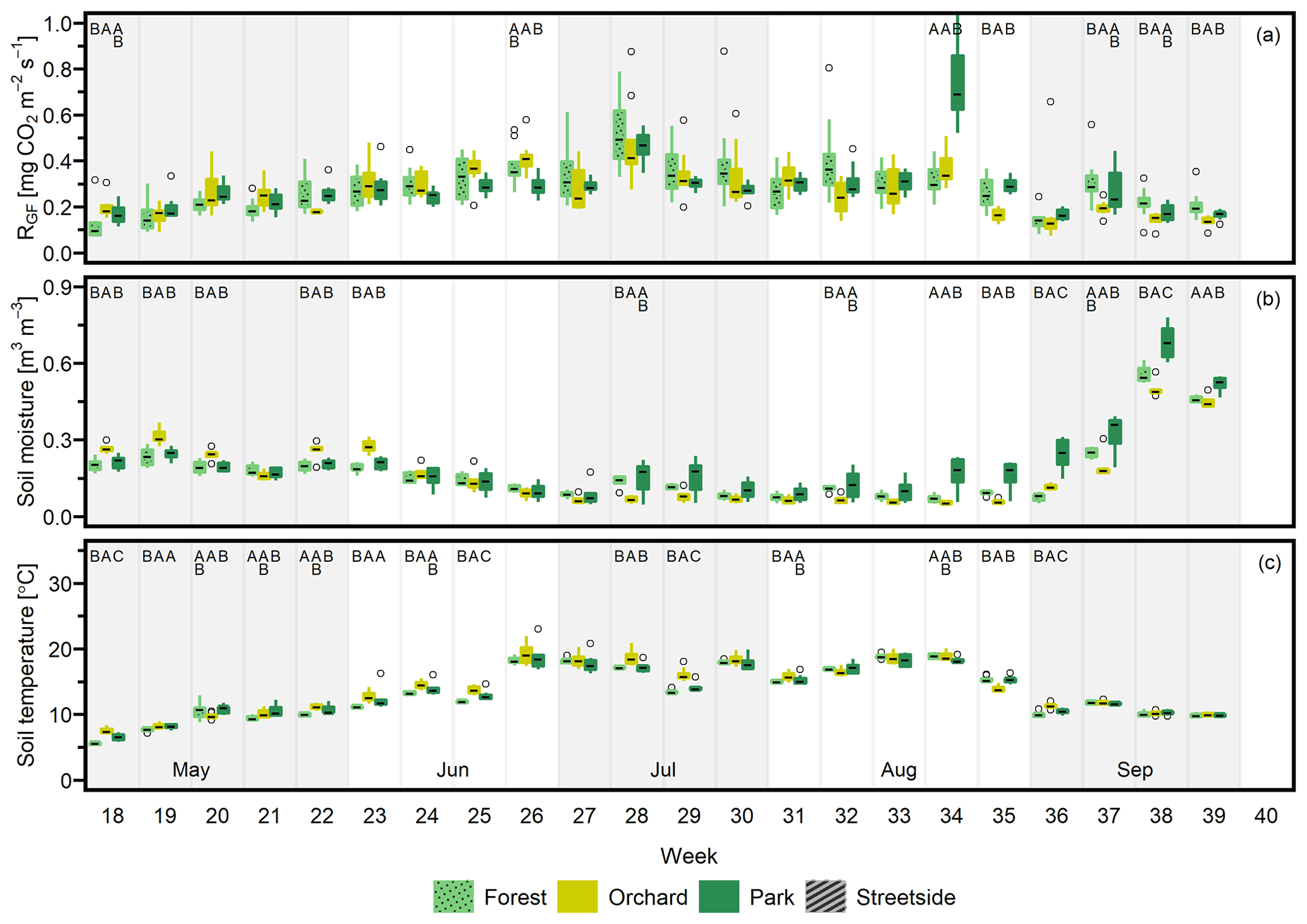
Figure D2 (a) Soil respiration (R_GF), (b) soil moisture (at 10 cm depth), and (c) soil temperature (at 10 cm depth) were measured weekly at three measurement sites (Forest, Orchard, and Park) in 2022. Here, boxes are arranged chronologically by week number and the sites are always presented in the order that is shown in the legend. Background shading indicates the month. Empty circles are outliers. Letters A–C denote statistically significant (p<0.05) differences between the sites. Note that Streetside was not measured in 2022.